transformation (i.e. linear combinations of all variables) in their antecedents. ... Multivariate rule-building expert system rules and neural network units perform ...
JOURNAL OF CHEMOMETRICS, VOL. 5 , 467-486 (1991)
FUZZY MULTIVARIATE RULE-BUILDING EXPERT SYSTEMS: MINIMAL NEURAL NETWORKS PETER B. HARRINGTON Department of Chemistry, Clippinger Laboratories, Ohio University, Athens, OH 45701-2979, U.S.A
SUMMARY A fuzzy multivariate rule-building expert system (FuRES) has been devised which also functions as a minimal neural network. This system builds rules from training sets of data that use feature transformation in their antecedents. The rules are constructed using the ID3 algorithm with a fuzzy expression of classification entropy. The rules are optimal with respect to fuzziness and can accommodate overlapped and underlapped clusters of data. The FuRES algorithm combines the benefits obtained from simulated annealing and gradient optimization, which provide robustness and efficiency respectively. FuRES classification trees support OR logic in their inference. The system automatically generates meaningful and consistent certainty factors during rule construction. Unlike other neural networks, FuRES uses local processing which furnishes qualitative information in the rule structure of its classification trees and variable loadings of the weight vectors. KEY WORDS
Expert system
Neural network
Fuzzy entropy
INTRODUCTION Supervised methods of pattern recognition are important aids for interpretation of complex data. Trends in automation and optimization of analytical instrumentation have increased the availability and intricacy of chemical information. Pattern recognition is a useful chemometric tool for obtaining information from data. Rule-building expert systems and neural networks are two emerging pattern recognition methods that may prove useful for automated on-line decision making. Rule-building expert systems construct classification trees composed of processing units. Each unit (i.e. rule) consists of an antecedent which tests whether a predetermined condition arises (i.e. IF part of the rule) and a consequent which directs the next rule to be applied or indicates a classification (i.e. THEN part of a rule). Univariate rule-building expert systems are commercially available and have been applied to a variety of chemical analysis. 1 - 4 Univariate expert systems approximate multivariate relations by a sequential univariate approach. Multivariate rule-building expert systems (MuRES) construct rules that use feature transformation (i.e. linear combinations of all variables) in their antecedents. Feature transformation is an alternative to feature selection (i.e. selecting a single key variable) and has been shown to be superior when linear combinations of variables are meaningful. For these cases multivariate expert systems are superior to univariate expert systems. MuRES has been improved by applying principles from fuzzy set theory. A fuzzy multivariate rule-building expert system (FuRES) has been devised which also is a
0886-9383/91/050467-20$10.00 0 1991 by John Wiley & Sons, Ltd.
Received 26 September 1990 Accepted (revised) 15 April 1991
468
P. B. HARRINGTON
minimal neural network (NN). FuRES accommodates relative distances in variable space, so that it accomplishes both modeling and discrimination synergistically. This property allows FuRES to define characteristic classifiers when classes are overlapped or contain outliers. Neural networks were designed to simulate biological nervous systems and are powerful pattern recognizers. 6 - 8 NN hardware architecture is composed of multiple parallel processing units that communicate by way of analog channels. However, they may be simulated on conventional sequential computers. NNs distribute their inference among all their processing units (i.e. neurons). The advantage of distributed processing is that if a processing unit is removed from the network, all conclusions will be degraded but still be supported. The disadvantage is that the mechanism of inference becomes obfuscated. Local processing is the antithesis of distributed processing. MuRES use local processing which differentiates them from NNs. With local processing each inference occurs at a single node (i.e. rule). Local processing has two fundamental benefits: the chain of inference may be traced and the rule structure provides inductive mapping of the data. An additional benefit is that multivariate decision trees have been shown to train more efficiently than neural networks.’ The disadvantage is that all conclusions depend on the rules along the chain of inference. If a rule is removed, all conclusions connected to that rule will be lost. Multivariate rule-building expert system rules and neural network units perform the same functions. They project their inputs on to a weight vector and perform a non-linear function on the projections. The non-linear operation used by MuRES is partitioning. Incorporation of a fuzzy paradigm by FuRES allows the algorithm to use the same non-linear function used by NNs. A FuRES rule and an NN unit are identical. Because the FuRES method is a novel configuration of a minimal NN and is a rule-building expert system, the terminology used in this paper will attempt to remain mutually consistent with the NN and expert system literature. Several exemplary test sets are used to demonstrate the features of FuRES classification, including the identification of polymers by laser ionization negative ion mass spectrometry (LIMS). Classification methods are often employed for LIMS data analysis because of the intricate nature of the data. A complex mixture of photothermal decomposition products may be produced by laser ablation and ionization. The relative yield of products depends on heat transfer, sample orientation, mass calibration and instrument configuration, which produces significant experimental errors. Industrial samples may be complex polymeric mixtures that further exacerbate the problem of direct mass spectral interpretation.
THEORY Many classification algorithms partition the data space into subspaces where all observations that have the same distinguishing property reside in the same partition. The dimension of a partition is one less than that of the spectra space. Thus if an object is measured over u variables, the data space is u-dimensional and the partitions will be ( u - 1)-dimensional hyperplanes. The hyperplane orientation can be defined by an orthogonal vector, which is referred to as a weight vector. The location of the hyperplane can be defined by the point of its intersection with the weight vector. Projection of data objects onto a weight vector is useful because the objects are mapped from a multidimensional space to a single dimension. The bias is defined as the point that partitions the projections and is the intersection of the hyperplane and weight vector. The antecedent of the rule determines whether a projection onto the weight vector is greater or less than the bias value. Selection of this point is crucial to the classification efficacy and depends
FUZZY MULTIVARIATE RULE-BUILDING EXPERT SYSTEMS
469
on the orientation of the hyperplane. Projections of data onto the weight vector are obtained by
where xk is the projection of observation d k , u is the number of variables of the observation and of the weight vector w and b is the bias value. The projection is corrected for the length of the weight vector. The necessity of this step will become apparent during the discussion of the logistic function. By subtracting b from the projection, the logic of the hyperplane separation is obtained from the sign of the projection. Therefore each rule is a binary classifier and each xk will have an attribute value of positive or negative. Previous researchers have determined the bias simultaneously with the hyperplane orientation by adding a component of constant value to each observation." Using an additional dimension to characterize the bias may deleteriously affect optimization methods, because the bias and the weight vector are strongly dependent. MuRES remedies this problem during optimization of a weight vector by determining the optimal bias for each evaluation of a trial weight vector. Likewise, FuRES determines the optimal bias for each gradient calculation. A minimal spanning tree of linear discriminants may be obtained by optimizing the entropy of classification, H(C I A ) . The ID3 algorithm, which is used by most rule-building expert systems, generates rules by minimizing H ( C I A ) . '','' The algorithm constructs a minimal spanning tree of rules that minimize the entropy of classification, H(C I A ) . H(C I A ) is given by
H ( C 1 a,) is the entropy for a given attribute aj, that is obtained by summing the conditional probability of a class c;, occurring for aj, over the number of classes, n. The probability p(ci I aj) is obtained by counting the number of observations of class i and dividing that number by the total number of observations with attribute j . Equation (3) gives the sum of the entropies for each attribute weighted by the prior probability that the attribute occurs. The number of attributes, m , is equal to two (the attributes are either positive or negative) and p ( a j ) is the number of observations with a given attribute divided by the total number of observations. H(CI A ) indicates more than the number of misclassifications of a rule. It also favors rules for which the misclassified points have the least influence, i.e. a lower p ( c ; /aj). Several problems exist for the MuRES algorithm. The first problem is group overlap. Groups of spectra in space may be overlapping and provide ill-conditioned rule construction. A converse situation is when group underlap occurs. The groups are well separated and an infinite number of hyperplanes exist which all have the same H(CI A ) . MuRES solves the problem of group underlap by maximizing the rule separation while maintaining a minimum entropy. After the rule is obtained, the critical value is centered at the median between the two closest projections with different attributes. Finding rules in spectra space may be confounded by local entropy minima.
470
P. B. HARRINGTON
Fuzzy set theory was developed by Zadeh in 1965 to accommodate inexact models of reality. l 3 Fuzzy set theory lends itself to inexact reasoning and may be considered an infinitevalued logic system. A crisp set consists of objects that either belong or do not belong to the set. Fuzzy sets have elements that may partially belong. Therefore the set boundary is not crisp and the set appears blurred or fuzzy. Perhaps one of the hindrances to the acceptance of fuzzy techniques in the United States is the connotation that fuzziness obscures information and is the same as haziness. This assumption is false, because crisp representation is encompassed by the fuzzy paradigm. 14,15 Fuzziness is a measure of uncertainty in representation and differs from probability which measures uncertainty in frequency of occurrence. Many concepts embodied in chemistry are inexact and fuzzy set theory has been applied to analytical chemistry. 16,17 Chemical compounds react to varying degrees and at varying rates. For example, when is a compound lipophilic or hydrophilic? Increasing the alkane portion of alkyl sulfonates gradually increases lipophilicity and decreases hydrophilicity. Alternatively, there are cases in chemistry for which set membership is crisp. For example, a molecule either has an ether functionality or it does not. FuRES encompasses these cases because it optimizes fuzziness within its rule construction. Fuzzy rules may be obtained by partitioning the spectra space into two fuzzy sets. For a partition that divides data into two fuzzy sets, the set membership values may be interpreted as a logistic function. The logistic function is 1.0
xA= I -0 + e-x'r
XA
+ U''
1.0
(4)
(6)
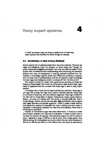
where X A is the degree of membership or truth in A , which varies between zero and unity, x is a variable that can vary between - 00 and 00, A C is the degree that A does not occur (the converse) and t is a variable analogous to thermodynamic temperature which controls the degree of fuzziness. The normalization of the weight vector in equation (1) is required so that the temperature will be defined. The variable t is referred to as the computational temperature and is given in the same unit as the spectral intensities. Temperature is a useful concept because it pertains to NNs, simulated annealing and thermodynamic entropy. This logistic function is plotted as a function of temperature and distance from the bias in Figure 1. Although many logistic functions may be used, this particular one has some advantageous properties. The fuzziness of the decision plane may be controlled by the temperature. As the temperature approaches zero, the logistic function approaches the crisp case for which binary logic is obtained. In contrast, as the temperature becomes large with respect to x , the logic will converge to a single value of 0.5, which is the maximum-entropy case where no partitioning occurs. The function is differentiable and provides symmetric blurring of the hyperplane. Fuzzy rule construction is similar to the method used by MuRES. The entropy of classification is the same but the conditional probabilities p(ci 1 aj ) differ. Instead of counting discrete objects t o obtain the conditional probability, the logistic values are counted: n
FUZZY MULTIVARIATE RULE-BUILDING EXPERT SYSTEMS
47 1
Each x,+is an object projected on to the multivariate rule (linear discriminant), X A is the fuzzy set membership value of x,+and ni is the number of objects in category i. A practical aspect of this fuzzy entropy calculation is that the fuzzy entropy approaches Shannon’s entropy (i.e. crisp entropy of classification) as the temperature approaches zero. 18,19 Blurring the response surface of the entropy function is useful because it smooths out the local minima. The blurring occurs not for the data points but for the fuzzy hyperplane. An object’s distance from the hyperplane is scaled by the temperature, which is constant during the positioning of the hyperplane and bias. Fuzzy partitioning of Fisher’s Iris Data is rendered in Figure 2 . 2o Note that the decision plane disappears at the bias and only objects outside the fuzzy decision space (darkened area) are completely (crisply) partitioned. Loglsltlc Functlon f(x)
= 1/(1+e-xn)
Figure 1. Plot of logistic values as function of computational temperature and attribute
Fuzzy Decision Plane Fisher’s Iris Data
-5
0.8 0.6 0.4
g
0.2 0.0
0 -
-0.2 -0.4
(v
t
g
..-
&
-0.6
-0.8 l
6.4
6.9
7.4
7.9
8.4
8.9
!
,
9.4
,
l
,
.
,
l
.
l
9.9 10.4 10.9 11.4
Principal Component 1 Figure 2. A rendition of a fuzzy partition of Fisher’s Iris Data at high temperature
472
P.B. HARRINGTON
The effects of temperature and bias value on entropy are examined with synthetic univariate data. Each datum was designated one of three class distinctions to produce three minimumentropy solutions. Figure 3(a) is a histogram of these data. The entropy at each temperature is plotted as a function of the bias value (i.e. to partition the data) in Figure 3(b). Three entropy minima are located between the class boundaries and are indicated by the arrows. At high temperatures only one minimum exists. The global minimum entropy may be found by following the trough of lowest fuzzy entropy on the bias value and temperature response
Synthetic Unlvarlate Data
(a)
Value of Entropy Mlnlma
1
0
8
Local Minima
16
24
32
40
48
56
64
72
80
Figure 3(a). Histogram of simulated data projections. The arrows indicate entropy minima
(b)
Univariate Partition
Figure 3(b). Plot of fuzzy entropy as a function of computational temperature, and location of the attribute for simulated data projections in Figure 3(a)
FUZZY MULTIVARIATE RULE-BUILDING EXPERT SYSTEMS
473
surface. Locating the lowest-entropy solution at a fixed low temperature would be confounded by these local minima. Entropy is a discrete function which changes values in steps. For this reason MuRES uses the non-linear simplex method, which is useful for optimizing discrete functions. 21 Simulated annealing is another effective method for optimizing discrete functions. 22 The fuzzy entropy expression is differentiable, which allows FuRES to use derivative optimization methods. The conjugate gradient optimization reported in Reference 23 is the optimization used by FuRES. This method was chosen because it has low memory overhead and rapid convergence. Derivative methods are advantageous because they require fewer function evaluations. Each function evaluation (i.e. determination of hyperplane orientation) is time-consuming, because the optimum bias value is determined. For large data sets (i.e. more than 100 observations and 30 variables) a considerable gain in temporal efficiency over the non-linear simplex optimization is obtained by FuRES. In addition, the logistic values are a function of the distance of the projections from the bias. Therefore minimizing the entropy of classification maximizes the separation of projections on the weight vector. Crisp classification trees often use a depth first search, for which a single path leads to the category designation at the leaf of the tree. Fuzzy classification may require searching the entire tree, because the path may be blurred and no clear distinctions exist between true and false consequents of a rule. Each rule partitions a set of observations into two fuzzy subsets, which are mutually complementary sets A and A' whose logistic values follow the relations given by equations (4)-(6). Therefore a hierarchy of fuzzy subsets is constructed. A certainty factor indicates the degree of fit of an object to its class value. Certainty factors are equal to the product of logistic values along the classification path (from the root to a leaf of the tree). For leaf nodes of the same class designation the certainty factors are added together, which provides AND/OR linkage of the rules. The certainty factors of observations used for training will always sum to unity because of the properties inherent in the logistic functions (4) and (5). Classifications for which the certainty factors will all be the same are obtained for observations that were not characterized by the training set. When the computational temperature is set too high, some of the projections may be located near the bias. The OR logic of the fuzzy classification tree becomes important for unresolved points (i.e. close to the bias). FuRES certainty factors accurately indicate the fit of an observation to the classification space. Once a weight vector and bias has been obtained, the training data are partitioned by each object's logistic value. Branching of the tree is controlled by these logistic values and a threshold ( K ) . The threshold is variable and determines which partitions an observation will be passed on to for further training. Observations are excluded from a partition if their logistic values are less than the threshold. A threshold value of 0.5 was used, because each observation was passed on to a single partition. If a threshold less than 0.5 is used, then redundancy is incorporated in the classification tree and convergence may not always be obtained. If a threshold greater than 0 . 5 is used, then observations may be removed from the training set when their projections are close to the bias. A figure of merit for evaluating classification accuracy is the root mean square error (ERMS) for each class prediction (i.e. a certainty value of 1 a 0 for the correct class and 0.0 for all others). The condition of the classification is very important when comparing methods that support multiple conclusions such as NNs and rule-building expert systems. For example, a correct classification may be ill-conditioned when it has a low certainty factor or it marginally exceeds the certainty of alternative conclusions. Alternatively, misclassifications may be obtained for which the certainty of a correct conclusion is marginally exceeded by one or more
474
P. B. HARRINGTON
other conclusions. E R Mcharacterizes ~ the condition of the classification and is given as
where pi,j is the predicted certain value for category j and observation i. The actual value Data Overlap
(a)
50
41 32
1
I
. ;
Class1 Class 2
A
23
-n
N
14
0)
A
A
A
A
~-
. . . -. . ' 1 = . .=.
5 -
Q
-
L
A
A
-
Q
A
A
-13 -22
-31 -40 -65.0
-53.3 -41.6
-29.9 -18.2 -6.5 5.2 Variable 1
A
A *
-
> -4
ai,j
A
m
A
16.9
28.6
40.3
52.0
Figure4(a). Plot of bivariate data where two groups of points overlap. 0 is the angle between the classifier and variable axis 1 (b)
Partition Overlap
Figure 4(b). Plot of fuzzy entropy as a function of computational temperature and B
FUZZY MULTIVARIATE RULE-BUILDING EXPERT SYSTEMS
475
for these cases will be 1.0 for the correct category of observation j and 0.0 for the other category certainty factors. The number of categories is c and the number of observations is n. The determination of the optimal computational temperature or degree of fuzziness is critical for rule generation. If the temperature is too high, a tree with many rules is obtained and the qualitative information is distributed among the rules. If the temperature is set too low, local minima, overlap and underlap become problems. The FuRES algorithm uses a conjugate gradient method to find the classifier with the lowest fuzzy entropy. 23 The minimization starts at a high temperature to remove the local minima. The classifier is iteratively refined at sequentially lower temperatures. The fuzzy entropy will decrease as the temperature is lowered until either data overlap or underlap occurs. If a rule misclassifies data, the fuzzy entropy will eventually increase as the temperature decreases. This behaviour occurs because misclassified points become influential as their certainty values increase. This case was simulated for two dimensions with normally distributed points about two group means. These points are shown in Figure 4(a). The angle of the weight vector with respect to variable 1 is given by 8. The fuzzy entropy obtained from each weight vector orientation was minimized with respect to the bias value. Figure 4(b) gives the fuzzy entropy as a function of temperature and 8, the angle of the classifier with respect to variable 1. If the data are underlapped, the entropy will not change below some temperature. Plots similar to Figures 4(a) and 4(b) are given for underlapped data in Figures 5(a) and 5(b). At the temperature for which the entropy stops decreasing, the gradient of the weight vector temperature response surface becomes a null vector. From a pragmatic perspective a constant temperature is a good terminating condition for the optimization. This underlapped example also demonstrates a case for which distances in the data space take precedence over a minimum crisp entropy. The FuRES algorithm terminates when the change in entropy with respect to temperature is less than or equal t o zero. The algorithm is initiated by finding a weight vector and bias that minimize the entropy of classification at a high temperature. If the initial temperature is too high, the bias of minimum entropy may be located outside the range of projection of the weight vector and no separation will occur. The entropy calculation has a penalty function which is used only when the bias does not partition the projections. The function is the distance between the bias and closest projection which is added to the entropy obtained in equation (3). Local minima may be obtained if the initial temperature is not sufficiently high. A good choice for an initial weight vector is the difference vector between the two objects. An adequate starting temperature is one-fourth the furthest distance in spectra space between two objects of different class distinction. Any large value may be used for the initial temperature so long as a penalty function given above is implemented in the entropy expression. The optimum weight vector and bias are iteratively refined by sequentially lowering the temperature. This process adds robustness to the optimization similar to that obtained by simulated annealing. 24 However, this method differs from simulated annealing which randomly evaluates points on a functions response surface. The FuRES optimization does not follow a random path but a path directed by the gradient of the weight vector. The temperature is lowered by dividing by an increment, instead of subtraction, because the temperature decrement will then be proportional to its value. Consequently, the temperature will drop rapidly when it is large and will asymptotically approach zero. The algorithm will not produce negative temperatures when it converges to a zero-entropy solution. The entropy will be lowered as the temperature is lowered even if the weight vector and bias remain constant until overlap or underlap occurs. Therefore the temperature is lowered until the change in entropy with respect to temperature is no longer positive.
476
P. B. HARRINGTON
Data Underlap
(a)
Class 2
1.75
0.50
1:
0.25
-
A
n
0.00 -0.25
-11.0
I
'
-8.8
"
-6.6
I
-4.4
'
I
-2.2
'
I
'
0.0
'
I
2.2
"
4.4
'
6.6
I
' 8.8
11.0
Variable 1
Figure 5(a). Plot of bivariate data where two groups of points underlap. B is the angle between the classifier and variable axis 1
Partition Underlap
(b)
0-0
Figure 5@).
Plot of fuzzy entropy as a function of computational temperature and 9
In summary, the algorithm continues to partition by rule logistic value until all the data of each leaf node consist of a single class. See the Appendix for a mathematical description of the algorithm. The temperature is lowered until the entropy for the optimum bias and weight vector no longer decreases. This step optimizes the rule fuzziness. For every evaluation of the weight vector gradient the optimum bias is determined. The certainty of an inference is determined by the product of an observation's logistic values produced by each rule from the root of the tree to each leaf. Inferences for the same class designation are summed. A fuzzy classification tree is obtained which is composed of rules that partition data into a hierarchy of fuzzy subsets.
F U Z Z Y MULTIVARIATE RULE-BUILDING EXPERT S Y S T E M S
477
EXPERIMENTAL A synthetic bivariate data set composed of two categories each composed of 40 observations is shown in Figure 6(a). This data set was constructed to demonstrate the value of multivariate expert systems when linear relationships exist among variables. Three clusters of randomly distributed observations were formed about three line segments: ten points of class w ( - 10.0,1.0), (-9.0,10-0), tenpointsof class m (3.0, l-O), (9-3,7.3); and 20points of class A (3.0,3-0), (9.3,10.3). Three clusters of two groups were used to furnish a data set that was not linearly separable. Observations were uniformly distributed within the variable 1 line segment range and normally distributed along the line segment with a standard deviation of 0.5 with respect to variable 2. Synthetic Bivarlate Data
(a) 10.26
A
Line S e g m e n t 1
Line S e g m e n t 2
8.46
7.56
--9 *
A *
6.66
m
A
&
'4
5.76 LP
4.86
3.96 3.06 2.16
A
1
L
AA
A
:
m I
m
I I
Line S e g m e n t 3
r
Rule: #2 Entropy: 0.00
Figure 6(b). FuRES classification tree for synthetic data set shown in Figure 6(a)
47 8
P. B. HARRINGTON
The LIMS analyses were performed on a Cambridge Mass Spectrometry, Ltd. (Cambridge, U.K.) Model LIMA 2A reflection mode laser microprobe instrument which has been described in detail elsewhere. 25 Fifteen negative ion laser microprobe mass spectra were obtained at laser irradiances which produced 100 times the threshold ion intensity. The irradiance of the pulsed laser output was approximately lo’* W cm-’ and the laser beam typically irradiates a 2-5 pm diameter area on the sample surface. A complete mass spectrum is obtained for each irradiated volume by employing a transient waveform digitizer in the detection circuitry. The Sony-Tektronix 390 AD transient digitizer employed in these analyses was operated at a sampling frequency of 60 MHz. Its record length was 4096 channels, which permitted acquisition of mass spectra over a mass range from 1 to 300 amu. Nylon 6 (A), nylon 12 (B), poly( 1,4-butylene)terephthalate (C), polycarbonate (D), polystyrene (E), polyimide S-11 (Dupont 1556) (1)’ polyimide S-09 (GE SPI 115) (2), polyimide S-24 (Hitachi PIX-1400) (3), polyimide S-10 (Toray LP-64) (4) and polyimide S-19 (Ciba Geigy Probimide 284) (5) samples were prepared by embedding beads of commercially available polymers in Spurr’s Epoxy Resin (Medium Hardness) (F) and microtoming 1 kni thick sections. These thin section samples were mounted on high-purity silicon substrates. The locations of the embedded polymers were readily apparent in the optical microscope of the laser microprobe, which allowed acquisition of mass spectra from the embedded polymer and not the Spurrs epoxy. Cleaned surgical knives were used to avoid contaminating the sample surfaces. The preparation of thin sections as well as the cutting or scraping of the top layers of the bulk specimens minimized the ion signals produced by chemicals such as mold release compounds and atmospheric contaminants. The poly(ethy1ene)terephthalate (Mylar 500D) (G) sample was provided in thin film form (- 0.5 mm thick) and was analyzed without any sample preparation. Replicate spectra from 15 different sample locations (except polyimide 4 which has 14 replicates) were obtained for each polymer. All mass channels with zero intensity were removed from the polymer data set, which reduced its number of variables to 247. The spectra were transformed using the autocorrelation method reported in Reference 26 and the zero-offset value from each spectrum was removed. The autocorrelation spectra were normalized to unit vector length and then scaled by the average of the group standard deviations. The spectra were compressed by eigenvector projection to produce abstract spectra composed of 30 scores which accounted for 98% of the total variance. The abstract spectra were used for MuRES and FuRES evaluation because they furnish an overdetermined representation of the data. For each of the five external validations of the polyimide spectra the evaluation spectra were not used in the calculation of the scale vector, principal components or classification trees. Calculations were performed on a 25 MHz 80386 IBM Model 70 PS/2 computer or a 25 MHz Everex Step 80486 computer. Four-byte floating point single-precision arithmetic was used with convergence tolerances set to 2.0 x for all evaluations, except for the FuRES evaluation of the polyimide data. The FuRES optimization was performed using 8 byte doubleprecision floating point arithmetic and derivatives were calculated with a precision of lo-’. Double precision improved the reliability of the derivative calculations and the stability of the algorithm for large data sets. Cooling was obtained by iteratively dividing the temperatures by a factor of 1 1. Internal and external validations of the classification were performed on the 80486 computer operating in native mode (linear address and 32 bit instructions). Protected mode programs were compiled using the Metaware Global Optimizing C Compiler 80386/486 vers. 2.3 and Phar Lap DOS Extender 386 vers. 2.2d. The 32 bit protected mode code was compiled using Metaware’s full optimization (-0)and 80486 (-486) options. Real mode
-
FUZZY MULTIVARIATE RULE-BUILDING EXPERT SYSTEMS
479
software was compiled using Borland’s Turbo C + + compiler vers. 1.0 and run under Microsoft’s DOS 4.01. The NN was a two-layer back-propagation network. The system contained 30 inputs, 30 hidden units and eight output units for the overdetermined data evaluation. For the underdetermined data evaluation the network was composed of 247 inputs, 247 hidden units and eight output units. The input units transfer each observation to the hidden units. These systems were trained until the total error converged for ten sequential epochs within a tolerance of 2.0 x The univariate expert system (Uni-ES) and MuRES are described in References 4 and 5 respectively. For the evaluations presented, these systems used certainty factors of 1 - 0 for each rule so that they would characterize a crisp classification limit. RESULTS AND DISCUSSION A synthetic bivariate data set was generated to demonstrate the benefits of FuRES inherent modeling characteristics. The data set was designed to demonstrate benefits of the FuRES algorithm in comparison to univariate expert systems and multivariate expert systems. The variables are correlated and feature transformation will be advantageous in rule construction. See Figure 6(a). Linear discriminant analysis (LDA) will perform deleteriously on these data because it attempts to separate the two classes of data using a single partition. Univariate expert systems approximate the correlations among variables with sequential rules, which results in a staircase-shaped partition between objects along line segment 2 and 3. In this case a single multivariate partition will more accurately characterize the clusters. MuRES will find a partition that is ill-conditioned with lower entropy which clusters the observation at (4.0, 1 2) along line segment 3 with points along line segment 1. FuRES groups a cluster of and of A together to separate the points along line segment 1 . Therefore the larger separation of points along line segment 1 in the data space is manifested in the structure of the FuRES classification tree structure in Figure 6(b). Rule # 1 generated by FuRES will have its weight vector nearly parallel to the variable 1 axis in Figure 6(a). This rule has a laiger entropy of 0.48 than the 0-45 entropy of the corresponding MuRES rule # 1. The MuRES rule obtains a lower entropy, but the projections with different attributes are not well separated. Internal validation (i.e. leave-one-out method) was used to evaluate classification accuracy. The proportions of correct classifications are given for each method as follows: LDA, 29/40; Uni-ES, 36/40; MuRES, 38/40; FuRES, 40/40. The second data set evaluation classified Fisher’s Iris Data. The sepal length, sepal width, petal length and petal width from Iris veriscofor and Iris virginicu were used to furnish a data set consisting of 100 observations. The Irissetosu data were not used because they can be easily separated by most classification methods. The objective of this evaluation was to measure classification efficiency and all methods were constrained to one discriminant (i.e. rule). Internal validation was used to measure classification performance. The multivariate methods all performed similarly with respect to the proportion of correct classifications: LDA, 95/ 100; FuRES 951100; MuRES 95/100; Uni-ES, 90/100. However, the FuRES method had a predicted E R Mof~0.24, which was smaller than the other values: LDA, 0.60; MuRES, 0.32; Uni-ES 0.45. The low ERMs-values demonstrate that the certainty factors developed by the FuRES algorithm are optimal. The two other expert systems approximate the crisp classification limit with each rule using a certainty factor of unity. Greater ERMs-values were obtained when the certainty factors described in the Uni-ES and MuRES references were used. 4 * 5
-
480
P. B. HARRINGTON
MuRES and FuRES were evaluated by their ability to classify organic thin film polymers. Figure 7 is a three-dimensional plot of the scores of the normalized and scaled autocorrelation spectra on the first three principal components, which accounted for 80% of the total variance. The underdetermined data set was composed of the normalized and scaled autocorrelation spectra. These data were compressed by projection onto 30 principal components to furnish the overdetermined data set. Figures 8(a) and 8(b) give the classification trees obtained from the MuRES and FuRES methods for the entire overdetermined data set. The FuRES rule # 3 is of higher entropy (1.34) than the MuRES rule # 3 (1 10). However, a greater separation between the projections with different attributes is obtained concomitant with the higher entropy. Note the clear separation in Figure 7 of the nylon 6 and polyimide spectra from the other polymers. Both MuRES and FuRES trees indicate this separation in rule # 1, but in rules # 2 and # 3 the importance of distance in the data space becomes readily apparent. In Figure 8(b) note that FuRES rule # 3 separates 3 and nylon 6 from the other poIyimides I , 2,4 and 5 , which are tightly clustered together. In Figure 8(a) the MuRES classification of rule # 3 has a much smaller separation, which is caused by the lower-entropy solution of clustering 3, A and 4 together. FuRES rule # 2 separates cluster G from B-F, which is caused by the large separation of many points in G from the other polymers. The external validation was used to compare classification methods for identifying the polyimides 1-5 from the other polymer classes A-F. Five different evaluations were conducted using each brand of polyimide spectrum in the model. A classification tree was built and classified a set of external data consisting of the other four brands of polyimide spectra. The multivariate expert systems were compared to a back-propagation NN and a univariate expert system. The classification methods were also evaluated to overfitting by using the autocorrelated mass spectral data across a range of offsets from 1 to 247. Figure 9(a) is a bar graph and table of the pooled results reported as the number of correct polyimide
O A
A B C
V
D
Negative Ion Polymer Scores From Autocorrelation Spectra
I
/
.e
Figure 7. Three dimensional plot of the first 179 polymer spectra scores on the first three principal components. The 3 designates a pure cluster of polyimide S-24. See the experimental section for legend
FUZZY MULTIVARIATE RULE-BUILDING EXPERT SYSTEMS
48 1
classifications out of the 296 total. Note that FuRES performs nearly perfectly: it missed only a single classification. The misclassified point had a certainty of 0.69 and the next best classification was correct with a certainty of 0.31. FuRES suffered a loss in performance for the underdetermined data but performed better than the other classification methods that trained with overdetermined data. Additionally, all rnisclassifications had low certainty factors for the misclassified spectra and the correct classification was indicated with comparable certainty. The worst case was a 0.88 certainty for the misclassification and 0.12 for the correct classification. Figure 9(b) gives the ERMSvalues for the different methods, which indicate the selectivity of the certainty factors with respect to classification performance. FuRES performs better with both overdetermined and underdetermined data sets. The efficiencies of MuRES and FuRES may be compared by using the average computation time for the five polyirnide evaluations. MuRES and FuRES were evaluated on a 25 MHz 80486 computer operating in 32 bit protected mode. For the overdetermined data (120 observations and 30 variables) MuRES required 34 min for each evaluation. The time required far classification of the evaluation spectra was negligible compared to training, which included the time elapsed during PCA and scaling. For the underdetermined data (120 observations and R U k 11 Entropy: 1.79
Rule: 12 [Entropy: 1.10
I
Rule:#4 1 Entropy: 0.46
r
Rule: 13
1 Entropy: 1.101
I Rule: 15
1
Rule: #6 Entropy: 0.46
Rule: #7 Entropy: 0.46
Figure 8(a). MuRES classification tree of entire LIMS autocorrelation polymer data set Rule: #I Entropy: 1.79
(b) Rule: P2 Entropy: 1.34
Rule: 13 Entropy: 1.15 Rule: Y5 Entropy: 0.84
Rule: 1 4 Entropy: 1.11
u
w
v
v
w
Rule: $6 Entropy: 0.00
w
Figure 8(b). FuRES classification tree of entire LIMS autocorrelation polymer data set
P . B. HARRINGTON
482
247 variables) MuRES required 27 h 29 min for each evaluation. FuRES required 11 a6 min for the overdetermined data and 2 h 14 min for the underdetermined data. Even though FuRES used double-precision arithmetic, a considerable gain in efficiency is obtained. The difference in training efficiencies is partially caused by the iteration of the optimizations. MuRES randomly varies the initial vertices and iterates the simplex optimization to find a global minimum entropy. This step may be considered similar to the iterated gradient optimization during temperature reduction used by FuRES. If the weight vector and attribute
Polyimide Classification Rate Autocorrelation Data
(0)
300
-
lumber of Correct Identifications ~~
250 200
-
150 -
100
-
50
0Overdetermined Underdetermined
Uni-ES
NN
MuRES
FuRES
242 132
219 246
277 231
295 278
Figure 9(a). Bar graph of the proportion of correct polyimide classifications obtained by external validation with 296 mass spectra
Polyimide Classification Error
(b)
Root Mean Square Prediction Error 0.6 0.5 0.4 0.3 0.2
0.1
0
PUnderdetermined G n
0.115
e
Classification Method
I
Overdetermined
Underdetermined
1
Figure 9(b). Bar graph of the ERMSof the polyimide classification obtained by external validation with 296 spectra. The values reported are averages for the five experimental runs
FUZZY MULTIVARIATE RULE-BUILDING EXPERT SYSTEMS
483
are optimal for a temperature decrement, then the gradient will be zero and the optimization is completed in one step. For a similar case the simplex method requires contraction around the optimum vertex, which is time-consuming, especially when the number of variables is large. A histogram of the spectra projected on rule # 2 from the FuRES classification tree is given in Figure 10. The bias has been subtracted from each projection, so the zero point is where the poly(ethy1ene)terephthalate spectra are partitioned from the other spectra. The stability of a rule may be ascertained by visual examination of rule score plots. SCORE PLOT ON RULE #2 1
14,
-a
-10
O
m
10
COMPONENT 2
Figure 10. Projections on FuRES rule #2; attribute has been subtracted so partition occurs at zero
Poly(ethy1ene)terephthaIate
(o) Y
- k' Q)
zb ' 4b
'
Lb
'
ab
.iba ' 120 ' 140
'
CT
'
110 ' 110 ' 260 ' a20 ' 240
I
M E Offset
Figure 11(a). A normalized and scaled autocorrelation mass spectrum of polyethylene terephthalate
Rule #2 Feature Weights
(b)
.-r
u)
c
Q) 5
c
C
Q)
> .c
-.m
Q)
U
L
a
'
-
'
rb ' ab
'
rbo ' & t o ' 140 ' l & n '
190 '
ado
'
220
M E Offset Figure 1 I(b). The weight vector used in rule # 2
'
240
P. B. HARRINGTON
484
A normalized and scaled autocorrelation spectrum for poly(ethy1ene)terephthalate is given in Figure ll(a). Note the similarity of the weight vector for rule # 2 that detects poly(ethy1ene)terephthalate in Figure 1l(b). The weight vector has extracted the significant features of the poly(ethy1ene)terephthalate spectra. Feature transformation combined with local processing of FuRES affords a useful qualitative and interpretive tool. In addition, the overall classification tree structure of FuRES yields inductive information regarding distances in the data space. CONCLUSIONS Although FuRES is a much faster algorithm than MuRES at training for large data sets, it is a slower algorithm than linear discriminant analysis or univariate expert systems. The computational overhead is offset by improved performance and the cheapening cost of computer power. FuRES is a complementary method to feature selection methods of pattern recognition. Including feature transformation as part of rule optimization is advantageous when linear combinations of the data variables are meaningful. FuRES has the advantages of both efficiency and efficacy over the MuRES method. The FuRES method determines the optimal degree of fuzziness and thereby can accommodate discrete cases. FuRES also constructs meaningful and stable certainty factors as part of its rule construction. FuRES inherently represents interclass distances in its rule construction, which makes it a softer discriminatory classifier and provides some of the benefits found in modeling methods. As a result, FuRES provides more stable rule formation and avoids classification by small or spurious features in the spectra. This quality imparts robustness for non-linearly separable cases. Although many similarities exist between FuRES and NNs, FuRES has the advantage that its rules furnish qualitative information which is amenable to visual interpretation. Further research directions include global optimization of classification tree entropy and non-fuzzy categorization of training data. ACKNOWLEDGEMENTS
This research was supported by Teledyne CME, Ohio University and the National Biscuit Company. Charles Evans and Associates, Filippo Radicati di Brozolo and Rober W. Odom are thanked for collecting and supplying the LIMS polymer data. Alan Hendricker, Peter Tandler, Busolo Wabuyele, Peng Zheng and Peter Rothman are thanked for their helpful comments and criticisms.
APPENDIX A: ALGORITHM FOR FINDING OPTIMUM t , w AND b
Initialization 1.
to = Max[[[dl - d2 111/2
2.
wo= Max [dl - d ~11]1dl - d2 I(
3.
bo = Min [H(CI to, WO)]
Select initial temperature to as the maximum distance between two observations d of different class designation. Select initial weight vector WO, as the differencenormalized distance between two observations of different class distinction. Obtain the best attribute bo for to and wo using line minimization program (10.2) of Reference 23.
FUZZY MULTIVARIATE RULE-BUILDING EXPERT SYSTEMS
485
Cooling
4. wn+1, b,+ 1 = Min [H(CI tn, wn,b,)l Find best wn+1 and bn+l is implicit by conjugate gradient minimization program (10.6) of Reference 23. g is cooling rate; typically values range between 1 * 1 5 . tn+1 = t n / g and 2-0. 6 . IF((Hn - H,+l)/(t,- tn+l)> 0 THEN GOT0 4 If the derivative is greater than zero go to step 4.
Entropy calculation internal in gradient calculation and line minimizations 7.
b, A.
I
= Min [H(C W n , tn)]
11
xk = (dkT*Wn)/ W n
1) - b n
D. H(CJaj) = - Cqr = l P(ci I aj) In
For every entropy calculation find line minimum b, by program (10.2) of Reference 23. Project data onto weight vector and subtract attribute value. Weight vector must be normalized so that t n is constant. Equation (1).
P(C,
I a,)
Equation (2).
Partitioning 8.
If If
xA < K , THEN omit
from partition A
< K , THEN omit from partition A'. K determines the rule redundancy; typical value is 0.5.
9. IF H ( C I t,, wn,b,) > 0 THEN continue partitioning process.
REFERENCES
1 . W. A . Schlieper, J . C. Marshall and T. L. Isenhour, J. Chem. Znfo. Comput. Sci. 28, 159 (1988). 2. M. P. Derde, L. Buydens, C. Guns, D. L. Massart and P. K. Hopke, Anal. Chem. 59, 1868-1871 (1987).
3. D. R. Scott, Anal. Chim. Acta. 223, 105-121 (1989). 4. P. B. Harrington, K. J . Voorhees, T. E. Street, F. R. di Brozoio and R. W. Odom, Anal. Chem. 61, 715 (1989). 5. P. B. Harrington, and K. J. Voorhees, Anal. Chem. 62, 729 (1990).
486
P. B. HARRINGTON
6. D. E. Rumelhart and J . L. McClelland, Parallel Distributed Processing, Vol. 1, MIT Press, Boston, MA (1986). 7. P. D. Wasserman, Neural Computing Theory and Practice, Van Nostrand Reinhold, New York (1989). 8. J . R. Long, V. G. Gregoriou and P. J . Gemperline, Anal. Chem. 62, 1791 (1990). 9. R. P. Brent, Report TR-CS-90-01,Computer Sciences Laboratory, Australian National University (January 1990). 10. G. L. Ritter, S. L. Lowry, C. L. Wilkins and T. L. Isenhour, Anal. Chem. 47, 1951 (1975). 1 1 . J . R. Quinlan in Machine Learning: A n Arti’cial Intelligence Approach, ed. by R. S. Michalski, J . G. Carbonell and T. M. Mitchell, p. 463, Tioga, Palo Alto, C A (1983). 12. B. Thompson and W. Thompson, Byte, 11, 149-158 (1986). 13. L. A. Zadeh, Info. Control. 8, 338 (1965). 14. B. Kosko, Info. Sci. 40, 165 (1986). 15. B. Kosko, IEEE Trans. Pattern Anal. Machine Intell. PAMI-8, 556 (1986). 16. 0. Mathias, Anal. Chem. 62, 797A (1990). 17. 0. Mathias, Chemometrics Intell. Lab. Syst. 4, 101 (1988). 18. C. E. Shannon, Bell. Syst. Tec. J. 27 (1948). 19. K. Eckshlager and V. Stephanek, Information Theory as Applied to Chemical Analysis, p. 70, Wiley, New York (1979). 20. R. A. Fisher, Ann. Eugenics 7 , 179-188 (1936). 21. J . A. Nelder and R. Mead, Compt. J. 7, 308 (1985). 22. S. Kirpatrick, C. D. Gelatt and M. P. Vecchi, Science, 220, 671-680 (1983). 23. W. H . Press, B. P. Flannery, S. A. Teukolsky and W. T. Vetterling, Numerical Recipes in C , Chap. 10, Cambridge University Press, Cambridge (1988). 24. J . H . Kalivas, N. Roberts and J . M. Sutter, Anal. Chem. 61, 2024 (1989). 25. T. Dingle, B. W . Griffiths, J . C. Ruckman and C. A. Evans Jr., Microbeam Analysis--1982, ed. by K. H. J. Heinrich, p. 365, San Francisco Press, San Francisco, C A (1982). 26. S . Wold and 0. H . J. Christie, Anal. Chim. Acta, 165, 51 (1984).