Neural Networks and Fuzzy Systems by Kosko.pdf - Google Drive

NEURAL NETWORKS AND FUZZY SYSTEMS

NEURAL NETWORKS AND FUZZY SYSTEMS A DYNAMICAL SYSTEMS APPROACH TO MACHINE INTELLIGENCE

Bart Kosko University of Southern California

~~

PRENTICE HALL, Englewood Cliffs, NJ 07632

Library of Congress Cataloging-In-Publication sample space" of all elementary outcomes of an experiment, then X is a "sure event," since P(X) = I. Then (1-19) implies that every probability P(A) equals the conditional probability P(A I X):

P(A)

P(A I X)

(1-20)

This identity reflects the general subsethood relationship

P(A)

S(X. A)

(1-21)

On the surface the subset hood relation ( 1-21) seems absurd. How can superset X belong to one of its own subsets'? How can the whole be part of one of its own parts'? X cannot totally belong to A unless X = A. But X can partiall.v belong

to A. The subsethood theorem in Chapter 7 proves that this partial containment depends directly on the overlap between X and Jl, the intersection X n !1. Figure 1.2 illustrates the Pythagorean geometry of the subsethood theorem in three dimensions. The shaded hyperrectangle defines F(2n), the fuzzy power set of lJ. The subsethood theorem relates S(A. TJ) to the magnitudes of A, B, and AnD: S(A. JJ)

M(A n lJ) M(/1)

----

(1-22)

The ratio in ( 1-22) resembles, behaves as, and generalizes the defining ratio ( 1-19)

FUZZINESS AS MULTIVALENCE

11

of conditional probability. ,1/ (A) denotes the fuzzy count of fit vector ;1: M(A)

Oj

+ · ·· + 0

11

(1-23)

M(A) generalizes the classical cardinality count, which sums only Is and Os. In the infinite case appropriate integrals replace summations. Equation ( 1-22) implies that the fuzzy entropy f,'(1i) of A equals the degree to which An A' contains its own superset 11 U A': E(A) = S(A u Jl'. An A'). In Figure 1.2. A= (3/4. 1/3. 1/6) and B = (1/4. 1/2. 1/3). Then the closest subset Bt to A that satisfies the total-subsethood condition

b!

~

bj, ... ' h~, ~ bll

(1-24)

*

corresponds to B' = (± ~), which also equals the pairwise minimum of J1 and R. Equation (1-24) generalizes ( 1-14) above. As discussed in Chapter 7, the subsethood theorem ensures this in general:

R'

AIR

(1-25)

Equation (1-23) implies that ]\J(A) = 15/12 = 5/4, and M(A n B) = 3/4. Then the subsethood theorem gives S(A, JJ) = (3/4)/(5/4) = 3/5 = 60%. Relative frequency provides the clearest example of between-set fuzziness. Suppose we flip a coin, draw balls from urns, or shoot at a target. The elementary events in X are trials. Each trial is successful or unsuccessful. So X does not possess fuzzy subsets in its event space (its sigma-algebra). Each coin flip results in a head or a tail, not something in between. Suppose A defines the subset of successful trials. If X contains n trials, then A corresponds to a vertex of J" and equals a bit vector of Is and Os. Suppose there are TLA successes out of n trials, where Is indicate successes and Os indicate failures. The event X equals total success, the bit vector of all Is. X contains n successes. Then, since A n X = A, the subsethood theorem ( 1-22) gives S(X. Jl)

(1-26)

Historically probability theorists have called the subsethood ratio in (1-26). or its limit, the "probability of success" or P(A). This adds only a cultural tag. The success ratio n 1/ 11 behaves no differently in its deterministic subsethood framework than it did in its "random" framework. The relative-frequency ratio still provides a stable estimate for probability values in our physical, engineering, economic. and gambling models. It still implies all the theorems it has always implied. But we cannot derive the relative-frequency ratio from between-set relationships if we deny the strict inequality ( 1-18) and insist that subsethood is two-valued. Bivalence forces us to assume the ratio as a theoretical primitive. Whether by design or by accident we have historically followed the bivalent path in mathematics for almost three thousand years. Bivalence has simplified our fonnal frameworks hut at a cost. It has led to logical paradoxes (bivalent contradictions). unexplained primitives, and "randomness" in a universe that seems to obey physical laws and where events have causes.

12


CHAP. 1

THE DYNAMICAL-SYSTEMS APPROACH TO MACHINE INTELLIGENCE: THE BRAIN AS A DYNAMICAL SYSTEM Several engineering and scientific disciplines study how adaptive systems respond to stimuli. Electrical engineers study the topic as signal processing, nonlinear filtering, coding theory, circuit design, and adaptive control. Computer scientists study it as algorithm and automata theory, computer design, robotics, and artificial intelligence. Mathematicians study it as function approximation, statistical estimation, combinatorial optimization, and dynamical systems. Philosophers study it as epistemology, causality, and action. Biologists study it as neuroscience. biophysics, ecology, evolution, and population biology. Psychologists study it as reinforcement learning, psychometrics, and cogmt1ve science. Economists study it as utility maximization, game theory, econometrics, and market equilibrium theory. Cultural anthropologists study it as culture. We shall emphasize electrical engineering as we seek general principles of how adaptive systems process inforn1ation. We call these principles machine-intelligence principles. We shall draw freely from the related fields of engineering and science. The tern1 artificial intelligence usually refers to the computer-scientific approach to machine intelligence. This approach emphasizes symbolic processing and tree search. AI has become the emblem for a popular computer-age view of the brain: brain = computer. This view ranges from classical science-fiction speculation (the computer HAL in 2001: A Space Odyssey) to proposed space-based weapons systems. We shall explore machine intelligence from a d_vnamical-systems viewpoint: brain = dynamical system. On this view a maple leaf falling to a potential-energy minimum on the ground better describes brain activity than does a computer executing instructions. The dynamical models we shall study are cast as large systems of differential or difference equations. The principles describe local or global interactions of nonlinear parallel processes. Some of these machine-intelligence principles and mechanisms may explain natural phenomena and processes. Some already extend our theoretical and mathematical knowledge. But ultimately they should help us build smarter machines. They should give rise to new computational devices-electrical, optical, molecular, plasma, ftuid, or other devices. In this sense machine intelligence becomes an engineering discipline. Nearly a half century ago Norbert Wiener 1194X] outlined the first incarnation of such a machine-intelligence engineering. Wiener called it cyhcrnetics. We shall focus our analysis on artificial neural networks and fuzzy systems. These new, related system~ represent broad classes of "machine-intelligent" adaptive systems. Chapters 2 through 6 describe neural network theory. Chapters 7 through II present a geometric theory of fuzzy sets and systems and its neural extension to adaptive fuzzy systems. The companion volume [Kosko, 1991] describes engineering applications of neural networks.

THE DYNAMICAL-SYSTEMS APPROACH TO MACHINE INTELLIGENCE

13

Neural and Fuzzy Systems as Function Estimators Neural networks and fuzzy systems estimate input-output functions. Both are trainable dynamical systems. Sample data shapes and "programs" their time evolution. Unlike statistical estimators, they estimate a function without a mathematical model of how outputs depend on inputs. They are model-ji-ee estimators. They "learn from experience" with numerical and, sometimes, linguistic sample data. Neural and fuzzy systems encode sampled information in a parallel-distributed framework. Both frameworks are numerical. We can prove theorems to describe their behavior and limitations. We can implement neural and fuzzy systems in digital or analog VLSI circuitry or in optical-computing media, in spatial-light modulators and holograms. Artificial neural networks consist of numerous, simple processing units or "neurons" that we can globally program for computation. We can program or train neural networks to store, recognize, and associatively retrieve patterns or database entries; to solve combinatorial optimization problems; to filter noise from measurement data; to control ill-defined problems; in summary, to estimate sampled functions when we do not know the form of the functions. The human brain contains roughly 10 11 or I 00 billion neurons [Thompson, 1985 J. That number approximates the number of stars in the Milky Way Galaxy, and the number of galaxies in the known universe. As many as 104 synaptic junctions may abut a single neuron. That gives roughly 10 1" or I quadrillion synapses in the human brain. The brain represents an asynchronous, nonlinear, massively parallel, feedback dynamical system of cosmological proportions. Artificial neural systems may contain millions of nonlinear neurons and interconnecting synapses. Future artificial neural systems may contain billions of real or virtual model neurons. In general no teacher supervises, stabilizes, or synchronizes these large-scale nonlinear systems. Many feedback neural networks can learn new patterns and recall old patterns simultaneously, and ceaselessly. Supervised neural networks can learn far more input-output pairs, or stimulus-response associations, than the number of neurons and synapses in the network architecture. Since neural networks do not use a mathematical model of how a system's output depends on its input-since they behave as model-free estimators-we can apply the same neural-network architecture, and dynamics, to a wide variety of problems. Like brains, neural networks recognize patterns we cannot even define. We call this property recognition without definition. Who can define a tree, a pillow, or their own face to the satisfaction of a computer pattern-recognition system'? These and most concepts we learn o.l1ensi,·elv, by pointing out examples. We do not learn them as we learn the definition of a circle. We abstract these concepts from sample data, just as a child abstracts the color red from observed red apples, red wagons, and other red things, or as Plato abstracted triangularity from considered sample triangles. Recognition without definition characteriLes much intelligent behavior. It en-

14


CHAP. 1

abies systems to generalize. Dogs, lizards, and slugs recognize multitudes of unforeseen, complex patterns without, of course, any ability to define them. Descriptive natural languages developed only yesterday in human evolution. Yet a great deal of modern philosophy, influenced by formal logic and behaviorist psychology, has insisted on concept definition preceding recognition or even discussion. Below we discuss how this insistence has helped shape the field of artificial intelligence and its emblem, the expert system. Neural networks store pattern or function information with distributed encoding. They superimpose pattern information on the same associative-memory medium-on the many synaptic connections between neurons. Distributed encoding enables neural networks to complete partial patterns and "clean up" noisy patterns. So it helps neural networks estimate continuous functions. Distributed encoding endows neural networks with fault tolerance and "graceful degradation." If we successively rip out handfuls of synaptic connections from a neural network, the network tends to smoothly degrade in performance, not abruptly fail. Computers and digital VLSI chips do not gracefully degrade when their components fail. Natural selection seems to have favored distributed encoding in brains, at least in sections of brains. Neural networks, and brains, pay a price for distributed encoding: crosstalk. Distributed encoding produces crosstalk or interference between stored patterns. Similar patterns may clump together. New patterns may crowd out older learned patterns. Older patterns may distort newer patterns. Crosstalk limits the neural network's storage capacity. Different learning schemes provide different storage capacities. The number of neurons bounds the number of patterns a neural network can store reliably with the simplest unsupervised learning schemes. Even for more sophisticated supervised learning schemes, storage capacity ultimately depends on the number of network neurons and synapses, as well as on their function. Dimensionality limits capacity. Biological neurons and synapses motivate the neural network's topology and dynamics. We interpret neurons as simple input-output functions, threshold switches for two-state neurons and asymptotic threshold switches for continuous neurons. We interpret synapses as adjustable weights. In neural analog VLSI chips [Mead, 1989], operational amplifiers model nonlinear neurons, and resistors model synapses. The overall network behaves as an adaptive function estimator. Indeed, commercial adaptive estimators are simple, usually linear, neural networks. These include antennae beam formers, high-speed modems, and echo-cancellers for longdistance telephone calls.

Neural Networks as Trainable Dynamical Systems Neural networks geomelri::.c computation. Network activity burrows a trajectory in a state space of large dimension, say !?". Each point in the state space defines a snapshot of a possible neural-network configuration.


15

The trajectory begins with a computational problem and ends with a computational solution. The user or the environment specifies the system's initial conditions, which define where the trajectory begins in the state space. In pattern learning, the pattern to be learned defines the initial conditions. In pattern recognition or recall, the pattern to be recognized defines the initial conditions. Most of the trajectory corresponds to transient behavior or computations. Synaptic values gradually change to learn new pattern information. Neuronal outputs fluctuate. The trajectory ends where the system reaches equilibrium, if it ever reaches equilibrium. In the simplest and rarest case, the equilibrium attractor is a fixed point of the dynamical system. Most popular neural networks converge to fixed points. In more complicated cases the equilibrium attractor is a limit cycle or limit torus. In Chapter 4 we discuss a crude method for storing discrete timevarying patterns as limit cycles in feedback networks. The equilibrium attractors are rohust or structurally stahle if small perturbations do not distort or destroy them. In general, and in most dynamical systems, the equilibrium attractor is aperiodic or chaotic. Once the network enters this region of the state space, it wanders forever without apparent structure or order. Yao and Freeman [1990] have used dynamical neural models and time-series data to argue that rabbit olfactory bulbs process odor inforn1ation with chaotic attractors. As discussed in the homework problems, the function .rk 1 1 = c:rk( I - .r!) behaves as a chaotic dynamical system for values of 1· near 4 and .r values in the open unit interval (0, 1). In Chapter 3 we discuss global Lyapunov functions for proving that certain feedback neural networks converge to fixed points from any initial conditions. Geometrically we can view the Lyapunov function as a surface sculpted by learned pattern information, as in Figure 1.3. Figure 1.3 illustrates the geometry of fixed-point stability in feedback neural networks. Patterns behave as rocks on the rubber sheet of learning. The patterns, as well as "spurious" or unlearned patterns, dig out attractor basins in the state space and tend to rest at the local Lyapunov minimum of the attractor. The Lyapunov sheet changes shape as the system learns new patterns. Input patterns C) rapidly classify to nearest stored neighbors as if they were ball bearings rolling into local depressions in a gravity field. In fixed-point attractor basins the state-trajectory balls stop at the local minima (or hover arbitrarily close to it). In limit-cycle attractors, the ball C) would rotate in an elliptical orbit inside the attractor basin. In limit-tori attractors, Q would cycle toroidally in the attractor basin, as if, in R 3 , winding around the surface of a bagel. In chaotic attractors. Q would wander aperiodically within the attractor region. In all these cases. the numher of attractor basins does not affect the speed of convergence, the rate at which CJ falls into the attractor basin. The dimensionality of the state space also docs not in principle affect the convergence rate. In practice, CJ converges exponentially quickly. This suggests that global stability may under! ic our biological neural net works· ability to rapidly recognize patterns. generate

16


CHAP. 1

L(X)

Pat tern Space

FIGURE 1.3 Global stability of a feedback neural network. Learning encodes the vector patterns P 1 , P2 , ••• by gradually sculpting a Lyapunov or "energy" surface in the augmented state space R"+ 1• Input vector pattern Q rapidly "rolls" into the nearest attractor basin, where the system classifies Q as a learned pattern P or misclassifies Q as a spurious pattern. Q's descent rate does not depend on the number of stored patterns.

answers, and exhibit appropriate muscle reflexes independent of the amount of pattern information in our brains. Computer-type storage devices tend to slow as the number and complexity of patterns stored in them increases. Mathematically we can describe the time evolution of the neural network by the (autonomous) dynamical system equation x(t)

f(x)

(l-27)

where the overdot denotes time differentiation. The state vector x(t) describes all neuronal and synaptic values of the neural network at time t. The neural network reaches steady state when (1-28) 0 holds indefinitely or until new stimuli perturb the system out of equilibrium. Neural computation seeks to identify the steady-state condition (l-28) with the solution of a computational problem, whether in pattern recognition, image segmentation, optimization, or numerical analysis. We can locally linearize f by replacing f with its Jacobian matrix of partial derivatives J. The eigenvalues of J describe the system's local behavior about an equilibrium point. For instance, if all eigenvalues have negative real parts, then the local equilibrium is a fixed point and the system converges to it exponentially


17

DECODING FEEDFORWARD

FEEDBACK

0

w

(J)

"z

> cr: w

a..

::::l

GRADIENT DESCENT LMS BACK PROPAGATION REINFORCEMENT LEARNING

RECURRENT BACKPROPAGATION

(J)

0

0 0

z w

RABAM 0

w

(J)

> cr: w

a..

::::l

VECTOR QUANTIZATION SELF-ORGANIZING MAPS COMPETITIVE LEARNING COUNTER-PROPAGATION

BROWNIAN ANNEALING SOLTZMANN LEARNING ABAM ART-2 BAM ~COHEN-GROSSBERG MODEL HOPFIELD CIRCUIT BRAIN-STATE-IN-A-BOX MASKING FIELD

(J)

z

::::l

ADAPTIVE RESONANCE ART-1 ART-2'

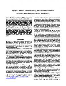
NEURAL NETWORK TAXONOMY Taxonomy of neural-network models. Source: "Unsupervised Learning in Noise," IEEE Trans. on Neural Networks, Volume 1, Number 1, March 1990. (© 1990 IEEE)

FIGURE 1.4

quickly. More abstractly, generalized eigenvalues or Lyapunov exponents describe the underlying dynamical contraction and expansion that may produce chaos. We can classify neural-network models depending on whether they learn with supervision (pattern-class information) and whether they contain closed synaptic loops or feedback. Figure 1.4 provides a rough taxonomy of several popular neuralnetwork models. Supervised feedforward models provide the most tractable, most applied neural models. We discuss these stochastic gradient systems in Chapter 5 and mention recent attempts to extend these supervised systems into the feedback domain. Unsupervised feedback models are biologically the most plausible, but mathematically the most complicated. These networks simultaneously learn and recall patterns. Both neurons and synapses change state when these systems learn and when they recall, recognize, or reconstruct pattern information. Chapter 6 proves global stability for many of these adaptive dynamical systems in the RABAM theorem. Unsupervised feedforward neural networks tend to converge to locally sampled pattern-class centroids, as discussed in Chapters 4 and 6, and in Chapter I of the companion volume 1Kosko, 1991 ].

18


CHAP. 1

Fuzzy Systems and Applications Fuzzy systems store banks of fuzzy associations or common-sense "rules." A fuzzy traffic controller might contain the fuzzy association "If traffic is heavy in this direction, then keep the light greeen longer." Fuzzy phenomena admit degrees. Some traffic configurations arc hcm·ier than others. Some green-light durations are longer than others. The single fuzzy association (HEAVY, LONGER) encodes all these combinations. Fuzzy systems are even newer than neural systems. Yet already engineers have successfully applied fuzzy systems in many commercial areas. Fuzzy systems "intelligently" automate subways; focus cameras and camcorders; tune color televisions; control automobile transmissions. cruise controllers, and emergency braking systems; defrost refrigerators; control air conditioners; automate washing machines and vacuum sweepers; guide robot-arm manipulators; invest in securities; control traffic lights, elevators, and cement mixers; recognize Kanji characters; select golf clubs; even arrange flowers. Most of these applications originated in Japan, though fuzzy products are sold and applied throughout the world. Until very recently, Western scientists, engineers, and mathematicians have overlooked. discounted, or even attacked early versions of fuzzy theory. usually in favor of probability theory. Below, and especially in Chapter 7, we examine this philosophical resistance in more detail and present a new geometrical theory of multivalued or "fuzzy" sets and systems. Fuzzy systems "reason" with parallel associative inference. When asked a question or given an input, a fuzzy system fires each fuzzy rule in parallel, hut to different degree, to infer a conclusion or output. Thus fuzzy systems reason with sets, "fuzzy" or multivalued sets, instead of bivalent propositions. This generalizes the Aristotelian logical framework that still dominates science and engineering. In one second a digital fuzzy VLSI chip may execute thousands, perhaps millions. of these parallel-associative set inferences. We measure such chip performance in FLIPS. fuzzy logical inferences per second. Fuzzy systems estimate sampled functions from input to output. They may usc linguistic (symbolic) or numeric samples. An expert may articulate linguistic associations such as (HEAVY, LONGER). Or a fuzzy system may adaptivcly infer and modify its fuzzy associations from representative numerical samples. In the latter case. neural and fuzzy systems naturally combine. The combination resembles an adaptive system with sensory and cognitive components. Neural parameter estimators embed directly in an overall fuzzy architecture. Neural networks "blindly" generate and reline funy rules from training data. Chapters X through II describe and illustrate these adaptive fuzzy systems. Adaptive fuzzy systems learn to control complex processes very much as we do. They begin with a few crude rules of thumb that describe the process. Experts may give them the rules. Or they may abstract the rules from observed expert behavior. Successive experience refines the rules and. usually. improves performance.

INTELLIGENT BEHAVIOR AS ADAPTIVE MODEL-FREE ESTIMATION

19

Chapter 9 applies this adaptive cognitive process to backing up a truck-andtrailer rig to a loading dock. (A supervised neural system can also solve this problem, though at much greater computational cost. So far the truck-and-trailer dynamical system has eluded mathematical characterization.) The fuzzy system quickly learns a set of governing fuzzy rules as it samples actual truck-and-trailer trajectories. Additional training samples improve only marginally the fuzzy system's performance. This property is better experienced than explained. As an exercise, you might try backing your car into the same parking space five times from five different starting positions.

INTELLIGENT BEHAVIOR AS ADAPTIVE MODEL-FREE ESTIMATION Below we discuss neural and fuzzy systems in more detail. First we examine the properties neural and fuzzy systems share with us and, more broadly, with all intelligent systems. These properties reduce to the single abstract property of adaptive model-free function estimation: Intelligent systems adaptil'ely estimate continuous ji111ctions from data without specifying mathematically how outputs depend on inputs. We now elaborate this thesis. A function f, denoted f: X --+ Y, maps an input domain X to an output range Y. For every element .r in the input domain X, the function f uniquely assigns the element y in the output range Y. We denote this unique assignment as iJ -= f(:r). f(.r) = .r 3 defines a cubic function. f(.ri, .r:2. :q) = (.rJ . .1:2. XT ~ x~) defines a "saddle" or hyperbolic-paraboloid vector function in physical or threedimensional space n'. Pressure is a function of temperature, mass of energy (c = nu· 2 ), gravity of mass, erosion of gravity, consumption of income. Functions define causal hypotheses. Science and engineering paint our pictures of the universe with functions. Humans, animals, reptiles, amphibians, and others also estimate functions. We all respond to stimuli. We associate responses with stimuli. We associate actions with scenarios, class labels with patterns, effects with causes. Equivalently, we map stimuli to responses. Mathematically, all these systems transform inputs to outputs. The transformation defines the input-output function f: X ____, Y. Indeed the transforn1ation defines the system. We can operatively characterize any system-atomic, molecular, biological. ecological. economic or legal, geological, galactic-by how it transforms input quantities into output quantities. We call system behavior "intelligent" if the system emits appropriate, problemsolving responses when faced with problem stimuli. The system may usc an associative memory embedded in the resistive network of an analog VLSI chip or embedded in the synaptic webs of its brain. Or the system may use a mathematical algorithm to search a decision tree. as in computer chess programs.

20


CHAP. 1

Generalization and Creativity Intelligent systems also generali:.e. Their behavioral repertoires exceed their experience. Eighteenth-century philosopher David Hume saw why: Intelligent systems associate similar responses with similar stimuli. Small input changes produce small output changes. Hence they estimate continuous functions. The pilot lands the airplane at night the same way if only a few of the runway lights are out or if the new runway differs only slightly from more familiar runways. The leopard stalks like prey in like ways in like circumstances. Each minnow in a school smoothly adjusts its swimming behavior to the position of its smoothly moving neighbors. Function continuity accounts for much novel or creative behavior, if not all of it. We call system behavior "novel" if the system emits appropriate responses when faced with new or unexpected stimuli. "Novel ideas," says behaviorist psychologist B. F. Skinner [ 1953], are "responses never made before under the same circumstances .... Novel contingencies generate novel fonns of behavior." Usually these new stimuli resemble known or learned stimuli, and our responses usually resemble known responses. Geometrically, when systems generalize or "create." they map stimulus balls to response balls. Consider a known stimulus-response pair (x. y). Stimulus x defines a point in the stimulus space S, the set of all possible stimuli for the problem at hand. In practice S often corresponds to the real Euclidean vector space R". Response y defines a point in the response space R, which may correspond to R 1'. Now imagine a stimulus ball Bx centered about stimulus x and a response ball By centered about response y. All the stimuli x' in Bx resemble stimulus x. The closer stimulus x' is to stimulus x, and hence the smaller the distance d(x'. x), the more x' resembles x. The responses y' in By behave similarly. Suppose y = .f(x) for some unknown continuous function .f: R" --+ H 1'. The function f defines the sampled system. Suppose further that f generates the response ball from the stimulus ball: By = .f(Bxl· So for every similar response y' in By, we can find some similar stimulus x' in Bx such that y' = f(x'). Formally f maps the stimulus ball onto the response ball. (We usc the tern1 "ball" loosely. Technically, .f(Bx) need not define an open ball in [{ 1'. Thus we measure By with a volume measure below in (1-29). The open mapping theorem in real analysis [Rudin. 1974] implies that all bounded onto linear transformations f map the open ball llx to some set in R 1' that contains the open ball By. where y = .f(x). At best we can only locally approximate most system transformations f as linear transformations.) Then we can measure the creativity Cu, (f) of system f, given the stimulus ball Bx, by the volume ratio

c11. (f)

(1-29)

where the \ · operator (Lebesgue measure) measures ball volume in !?" or H1'. CIJ,, crude ~1s it is, captures many intuitions. It also resembles a spectral transfer function.


21

Consider the extreme cases of infinite and zero creativity. For a fixed nondegenerate response ball By, as the stimulus ball Bx contracts to x, the creativity measure CIJ, (f) increases to infinity. (The point x has zero volume.) Cu, (f) also increases to infinity if the stimulus ball is constant and nondegenerate but the response ball By expands without bound as its radius approaches infinity. In both cases an infinitely creative system emits infinitely many responses when presented with, in the first case, a vanishingly small number of stimuli or, in the second case, a fixed set of stimuli. Infinite creativity need not represent infinite problem solving. The reinforcing environment selects "solutions" from our varied or creative responses. Most creative solutions are impractical. We can emit creative responses without solving problems or contributing to our genetic fitness. Sometimes we call these responses "art" or "play." At the other extreme, zero creativity occurs when the response ball By vanishes or when the stimulus ball expands without bound as its radius grows to infinity. In the first case the system f is a constant function. It maps all stimuli in Bx to a single value y in R~'. Such an f is "dumb"' or "dull." In the second case, for an infiniteradius stimulus ball Bx, the stimuli overwhelm the system's response repertoire. Such systems resemble classical pattern-recognition devices that are sensitive only to well-defined, well-centered patterns (faces, zip codes, bar codes). Small variations in input provide the simplest novel stimuli. The physical or cultural environment may produce these variations. Or we may systematically produce them as grist for our analytical mill. We may vary stimuli to solve a crossword puzzle, to fit physical variables to astronomical data, or to formulate and resolve a mathematical conjecture. We are all forward-looking creatures. We tend not to see the gradual causal chains that precede our every action, idea, and innovation. Even Beethoven's Fifth Symphony appears less a discontinuity when we examine Beethoven's notebooks and a variety of preceding musical compositions by him and by other composers. Variation and selection drive biological and cultural evolution. Physical and cultural environments drive the selection process. Function continuity, and other factors, drive variation. Nature and man experiment with local variations of input parameters. This generates local variations of output parameters. Then selection processes filter the new outputs. More accurately, they filter the corresponding new systems. We call the new systems "winners" or "fit" if they pass through the selection filters, "losers" or "unfit" if they do not pass through. Variation and selection rates may vary, especially over long stretches of geological or cultural time. Different perturbed processes unfold at different speeds. So some evolutionary stretches appear more "punctuated" than others [Gould, 19R0l. This means some measures of change-ultimately time derivatives-are nonlinear. It does not mean that the underlying input-output functions arc discontinuous.

22


CHAP. 1

Learning as Change Intelligent systems also learn or adapt. They learn new associatiOns, new patterns, new functional dependencies. They sample the ftux of experience and encode new information. They compress or quantize the sampled ftux into a small, but statistically representative, set of prototypes or exemplars. Sample data changes system parameters. "Learning" and "adaptation" are linguistic gifts from antiquity. They simply mean parameter change. The parameters may be numerical weights in an innerproduct sum, average neurotransmitter release rates at synaptic junctions, or gene (allelic) frequencies at chromosomal loci in populations. "Learning" usually applies to synaptic changes in brains or nervous systems, coefficient changes in estimation or control algorithms or devices, or resistor changes in analog VLSI circuitry. Sometimes we synonymously apply "adaptation" to the same changing parameters. In evolutionary theory "adaptation" applies to positive changes in gene frequencies [Wilson, 19751. In all cases learning means change. Formally, a system learns if and only if the system parameter vector or matrix has a nonzero time derivative. In neural networks we usually represent the synaptic web by an adjacency or connection matrix M of numerical synaptic values. Then learning is any change in any synapse: M

i=

0

( 1-30)

We can learn well or learn badly. But we cannot learn without changing, and we cannot change without learning. Learning laws describe the synaptic dynamical system, how the system encodes information. They determine how the synaptic-web process unfolds in time as the system samples new information. This shows one way that neural networks compute with dynamical systems. Neural networks also identify neural activity with dynamical systems. This allows the systems to decode information. In principle we can harness any dynamical system to encode and decode some information. We can view a kinetic swirl of molecules, a joint population of lynxes and rabbits, and a solar system as systems that transfonn input states to output states. Initial conditions and perturbations encode questions. Transient behavior computes answers. Equilibrium behavior provides answers. In the extreme case we can even view the universe as a dynamical-system "computer." A godlike entity may choose Big-Bang initial conditions, and there are infinitely many, to encode certain information or to ask certain questions. The dynamical system computes as the universe expands transiently. Universal equilibrium behavior could represent the computational output: a heat-death pattern or perhaps a periodic or chaotic oscillation of expansion and contraction. Consider mowing a lawn of green grass. The mower "teaches" the lawn the short-grass pattern. The lawn consists of a parallel field of grass blades. Grass blades learn what they are cut. The lawn behaves as a semipennanent, yet plastic, infonnation-storage medium. It tolerates faults and distributes cut patterns over


23

large numbers of parallel units. We can mow our name in the lawn, and read or decode it from a rooftop. In principle we can encode all known information in a sufficiently big lawn. Eventually the lawn will forget this infonnation if we do not resample comparable data. if we do not re-mow the lawn to a similar shape. Ultimately learning provides only a means to some computational end. Neural networks learn patterns or functions or probability distributions to recognize future patterns, filter future input streams of data, or solve future combinatorial optimization problems. Fuzzy systems learn associative rules to estimate functions or control systems. We climb the ladder of learning and kick it away when we reach the roof of computation. We care how the learned parameter performs in some computational system, not how it was learned, just as we applaud the piano recital and not the practice sessions. Neural and fuzzy systems ultimately learn some unknown probability (subsethood) function p(x). The probability density function p(x) describes a distribution of vector patterns or signals x, a few of which the neural or fuzzy system samples. When a neural or fuzzy system estimates a function f: X ---+ Y, it in effect estimates the joint probability density 11(x. y). Then solution points (x. f(x)) should reside in high-probability regions of the input-output product space X x Y. We do not need to learn if we know p(x). We could proceed directly to our computational task with techniques from numerical analysis, combinatorial optimization, calculus of variations, or any other mathematical discipline. The need to learn varies inversely with the quantity of infonm1tion or knowledge. Sometimes the patterns cluster into exhaustive decision classes JJ 1 ••••• lh. The decision classes may correspond to high-probability regions or "mountains." (If the pattern vectors arc two-dimensional, then p(x) defines a hilly surface in three-dimensional space U1 .) Then class boundaries correspond to low-probability regions or '"valleys" on the probability surface. SuJ)('ITiscd learning uses class-membership infonm1tion. Unsupcn·iscd learning does not. An unsupervised learning system processes each sample x hut does not "know" that x belongs to class JJ, and not to class D.~. Unsupervised learning uses unlabelled samples. Neither supervised nor unsupervised learning systems assume knowledge of the underlying probability density function p(x). Suppose we want to train a speech-recognition system at an international airport. We want the German lighthulh to light up when someone speaks German to the speech-recognition system. the Hindi lightbulb to light up when someone speaks Hindi. and so on. The system learns as we feed it training waveforms or spectrograms. We supervise the learning if we label each training sample as German, Hindi, Japanese, etc. We may do this to compute an error. If the English lightbulb lights up for a (Ierman sample, we may algorithmically punish the system for this m isc lassi tication. An unsupervi\ed system learns only from the ritw training samples. We do not indicate language cia\.\ label\. Unsupervised systems adaptively cluster like patterns \\ ith Iike patterns. The speech-recognition \ystem gradually clumps German speech

24


CHAP. 1

patterns together. In competitive learning, for instance, the system learns class centroids, centers of pattern mass. Unsupervised learning may seem difficult and unreliable. But most learning is unsupervised, since we do not know accurately the labels of most sample data, especially in real-time processing. Every second our biological synapses learn without supervision on a single pass of noisy data.

Symbols vs. Numbers: Rules vs. Principles We all share another property: We cannot articulate the mathematical rules that describe, if not govern, our behavior. We can ask a violinist how she plays, and she can tell us. But her answer will not be a mathematical function. In general her answer will not enable us to reproduce her behavior. All lifeforms recognize vast numbers of patterns. The most primitive patterns relate to how an organism forages, avoids predators, and reproduces [Wilson, 1975]. On this planet only man articulates rules, and he articulates very few. We articulate some rules in grammar, common law, and science ("physical laws"). Yet all our natural languages, living and dead, and all our systems of law have culturally evolved without conscious design and not in accord with articulated principles [Hayek, 1973]. To some extent this also holds for our accumulated knowledge of medical, biological, and social science. There have been exceptions, and the exceptions have helped create the field of artificial intelligence. Last century linguists developed the articulated language Esperanto. Mathematician Giuseppe Peano similarly devised the language lnterlingua. A few fans still learn and speak Esperanto and lnterlingua, but far fewer speak them than speak Latin. This century computer scientists have consciously created the many computer programming languages. Today programmers frequently use C, Pascal, and even Fortran, and infrequently use Algol and Jovial. Computer scientists developed artificial intelligence in large part around the computer language Lisp, or fist processing, and more recently around Prolog, or logic programming. Lisp and Prolog process symbols and lists of symbols. Symbolic logic, the bivalent propositional and predicate calculi, underlies their processing structure.

Expert-System Knowledge as Rule Trees AI systems store and process propositional rules. The rules are logical implications: IF A, THEN n. They associate actions 13 with conditions A. The rule antecedents and consequents correspond to step functions defined on their universes of discourse. One part of the input space activates or "fires" A as true. and the other part does not activate k Collections of rules define "knowledge bases" or "rulebases." The rule A _, IJ locally structures the knowledge of .1 and J3 as a logical implication. The


25

knowledge base globally structures the rules as an acyclic tree (or forest). The logical-implication paths A ----+ B ----+ C ____, D ----+ ••• flow from the tree's root nodes or antecedents to its leaf nodes or consequents. The term knowledge hase stems from the computer-scientific term database. Because of the tree structure of knowledge bases, we might more accurately call them knmvledge trees. Chapter 4 discusses fuzzy cognitive maps, which use feedback and vector-matrix operations to convert knowledge trees to knowledge networks. Knowledge engineers search the knowledge tree to enumerate logical paths. Path enumeration defines the inference process. Forward-chaining inference proceeds from knowledge-tree antecedents to consequents. Backward-chaining inference proceeds from consequents or observations to plausible antecedents or hypotheses. Forward-chaining inference answers what-if questions. It derives effects from causes. Backward-chaining inference answers why or how-come questions. It suggests causes for observed effects. Path-enumeration complexity increases nonlinearly with the number of rules stored. Real-time path enumeration in large knowledge trees may be combinatorially prohibitive, requiring heuristic or approximate search strategies [Pearl, 1984 ]. Knowledge engineers acquire, store, and process the bivalent rules as symbols, not as numerical entities. This often allows knowledge engineers to rapidly acquire structured knowledge from experts and to efficiently process it. But it forces experts to articulate the propositional rules that approximate their expert behavior, and this they can rarely do.

Symbolic vs. Numeric Processing Symbolic processing fits naturally in the brain-as-computer framework. Language strings model thoughts or short-term memory. Rules and relations between language strings model long-term memory. Programming replaces learning. Logical inference replaces time evolution and nonlinear dynamics. Feedforward flow through knowledge trees replaces feedback equilibria. But we cannot take the derivative of a symbol. We require a sufficiently continuous function. Symbol processing precludes mathematical analysis in the traditional senses of engineering and the physical sciences. The symbolic framework allows us to quickly represent structured knowledge as rules, but prevents us from directly applying the tools of numerical mathematics and from directly implementing AI systems in large-scale integrated circuits. Figure 1.5 provides a taxonomy of model-free estimators. The taxonomy divides the knowledge type into structured (rule-like) and unstructured types and divides the framework into symbolic and numeric. All entries define model-free estimators, because users need not state how outputs depend mathematically on inputs. Figure 1.5 outlines the advantages and disadvantages of machine-intelligent systems. AI expert systems exploit structured knowledge, when knowledge engi-

26


CHAP. 1

FRAMEWORK

w

STRUCTURED

SYMBOLIC

NUMERICAL

AI EXPERT SYSTEMS

FUZZY SYSTEMS

CC}

0

w

....J

s: 0

z

UNSTRUCTURED

NEURAL SYSTEMS

~

FIGURE 1.5 Taxonomy of model-free estimators. User need not state how system outputs explicitly depend on inputs.

neers can acquire it, but store and process it outside the analytical and computational numerical framework. Neural networks exploit their numerical framework with theorems, efficient numerical algorithms, and analog and digital VLSI implementations. But neural networks cannot directly encode structured knowledge. They superimpose several input-output samples (x,, YI ), (x2, Y2), ... , (x y on a black-box web of synapses. Unless we check all input-output cases, we do not know what the neural system has learned, and in general we do not know what it will forget when it superimposes new samples (xA. yk) atop the old. We cannot directly encode the common-sense traffic-light rule "If traffic is heavy in one direction, keep the light green longer in that direction." Instead we must present the system with a sufficiently large set of input-output pairs, combinations of numerical traffic-density measurements and green-light duration measurements. 11 ,

11 , )

Fuzzy Systems as Structured Numerical Estimators Fuzzy systems directly encode structured knowledge but in a numerical framework. We enter the fuzzy association (HEAVY, LONGER) as a single entry in a FAM-rule matrix. Each entry defines a fuzzy associative memory (FAM) "rule" or input-output transformation. In Chapter 8 we discuss the fuzzy control of an inverted pendulum. Figure 1.6 shows a bank of FAM rules sufficient to control an inverted pendulum. (}, 6.(}, and v define fuzzy variables. Fuzzy variables (} and 6.(} define the system's state variables. The angle fuzzy variable 0 measures the angle the pendulum shaft makes with the vertical and ranges from -90 to 90. The angular-velocity fuzzy 6.(} variable measures the instantaneous rate of change of angle values. In practice it measures the difference between successive angle values. Output fuzzy

27


e NM NS

ZE

PS

PM

NM NS ~e

ZE PS PM

FIGURE 1.6 Bank of FAM rules to control an inverted pendulum. Each entry in the FAM matrix defines a fuzzy association between output fuzzy sets and paired input fuzzy sets.

NL

'

- 9o

NM

NS

ZE

PS

PM

o 3

PL

8

'

9o

FIGURE 1.7 Seven trapezoidal fuzzy-set values assumed by fuzzy variable e. Each value of 11 belongs to each fuzzy set to some, but usually zero, degree. The exact value 3 belongs to the zero fuzzy number ZE to degree 0.6, to the positive small fuzzy number PS to degree 0.2, and to positive medium PM to degree 0.

variable v measures the current to a motor controller that adjusts the pendulum shaft. Each fuzzy variable can assume five fuzzy-set values: Negative Medium (NM), Negative Small (NS), Zero (ZE), Positive Small (PS), and Positive Medium (PM). The entry at the center of the FAM matrix defines the steady-state FAM rule: "IF (} = ZE AND 6.(} = ZE, THEN v = ZE." We usually define the fuzzy-set values NM, .... PM as trapezoids or triangles over regions of the real line. For the fuzzy angle variable (}, we can define ZE as a narrow triangle centered at the zero value in the interval [-90, 90]. Then the angle value 0 belongs to the fuzzy set ZE to degree 1. The angle values 3 and -3 may belong to ZE only to degree 0.6. Figure 1.7 shows seven trapezoidal fuzzy-set values assumed by fuzzy variable e. Fuzzy systems allow users to articulate linguistic FAM rules by entering values

28


CHAP. 1

in a FAM matrix. Once a fuzzy engineer defines variables and fuzzy sets, the engineer can design a prototype fuzzy system in minutes. Chapter 8 shows that a large neural-type matrix encodes each FAM rule. When fuzzy variables assume fuzzy subsets of the real line, as when we define ZE as a triangle centered about 0, then these associative matrices have uncountably infinite dimension. This endows each FAM rule with rich structure and "memory capacity." FAM systems do not add these matrices together, which avoids neural-type crosstalk. A virtual representation scheme allows us to exploit the coding and capacity properties of these infinite matrices without actually writing them down. This holds for binary input-output FAMs (BIOFAMs), which includes all fuzzy systems used in commercial applications. BIOFAMs accept nonfuzzy scalar inputs, such as fJ = 15 and 6.0 = -I 0, and generate non fuzzy scalar outputs, such as l' = -3.

Generating Fuzzy Rules with Product-Space Clustering Neural networks can adaptively generate the FAM rules in a fuzzy system. We illustrate this in Chapters 8 through II with the new technique of unsupervised product-space clustering. Synaptic vectors quantize the input-output space. Clustered synaptic vectors track how experts associate appropriate responses with input stimuli. Each synaptic cluster estimates a FAM rule. The experts who generate the input-output data need not articulate the FAM rules. They need only behave as experts. The key geometric idea is cluster equals rule. Consider the input-output product space of the inverted-pendulum system. There are two input variables and one output variable, so the input-output product space equals I(' (in practice a three-dimensional subcube within !? 3 ). Each inputoutput triple (fJ. D.B. 1·) defines a point in R 1. The time evolution of the invertedpendulum system defines a smooth curve or trajectory in R 3 • As the fuzzy system stabilizes the inverted pendulum to its vertical position, the trajectory may spiral into the origin of R 3 , where the above steady-state FAM rule keeps the system in equilibrium until perturbed. Each fuzzy variable can assume five fuzzy subsets of the .r. y, or.~ coordinate axes of R 1 . The Cartesian product of these fuay subsets defines 125 ( 5 x 5 x 5) FAM cells in the input-output product space 1?1 . Most system trajectories pass through only a few FAM cells. We show in Chapter 8 that these FAM cells equal FAM rules because the FAM cells equal fuzzy Cartesian products, and the uncountably infinite entries in the associative matrices correspond to these Cartesian products. So a FAM rule equals an associative (fuzzy Hebb) matrix, which equals a fuzzy Cartesian product, which equals a FAM cell. Unsupervised neural clustering algorithms efficiently track the density of inputoutput samples in FAM cells. We need only count the number of synaptic vectors in each FAM cell at any instant to estimate, and to weight, the underlying FAM rules used by the expert or physical process that generates the input-output data. This produces an wlaJIIil·e histogra111 of FAM-cell occupation. Chapters 8 through II apply


29

the adaptive product-space clustering methodology to inverted-pendulum control, backing up a truck-and-trailer in a parking lot, and real-time target tracking. Suppose a system contains n fuzzy variables, and each fuzzy variable can assume 111 fuzzy-set values. This defines rn 11 FAM cells in the input-output product space R 11 • Different fuzzy variables can assume different types and different numbers of fuzzy-set variables. So in general there arc m 1 x · · · x 7rl 11 FAM cells. Suppose 11 = 111 = 3. Suppose the fuzzy sets arc low, medium, and high and have bounded extent. Then a Rubik 's cube represents the input-output product space partitioned into 27 FAM cells if the fuzzy sets do not overlap. In general FAM cells have nonempty but fuzzy intersection. If we define n fuzzy variables, each with m fuzzy-set values, then there are 2' 11 possible fuzzy systems. Expert articulation, fuzzy engineering, and adaptive estimation produce only a small fraction of the total number 2' 11 " of possible fuzzy systems. Different fuzzy-set definitions and different encoding or decoding strategies ("infercncing" techni4ues) produce different classes of 2 11 ' ' possible fuzzy systems.

Fuzzy Systems as Parallel Associators Fuzzy systems store and process FAM rules in parallel. Mathematically a fuzzy system maps points in an input product hypercube (possibly of infinite dimension) to points in an output hypercube. Fuzzy systems associate output fuzzy sets with input fuzzy sets, and so behave as associative memories. Unlike neural associative memories. fuzzy systems do not sum the associative matrices that represent FAM rules. Neural networks sum throughputs. Fu::y systems sum outputs. Summing outputs avoids crosstalk and achieves modularity. We can meaningfully look inside the black box of a fuzzy model-free estimator. Figure I .8 displays the generic fuzzy system architecture for a single-input. single-output FAM system. Fuzzy inference computes the output fuzzy sets Uj, weights them with the scalar weights u·.~, and sums them to produce the output fuzzy set B: lJ

L u·.~u;

( 1-3 I)

In principle in (I -3 I) we sum over all 111 11 possible FAM rules. since most rules have weight u·, = 0. Chapter 8 discusses the mechanism of the two types of fuzzy inference, correlation-product and correlation-minimum inference. Adapti1·c jir:.:y systems use sample data and neural or statistical algorithms to choose the coefficients u·.~ and thus to define the fuzzy system at each time instant. Adaptation changes the system structure. Geometrically, a time-varying betweencube mapping defines an adaptive fuzzy system. In the simplest case, if the input fuzzy sets define points in the unit hypercube ! 11 , and the output fuzzy sets define points in the unit hypercube [I'. then transformation S defines a fuzzy system if S maps !" to 11'. S: l" -~ ! 1'. Then S associates fuzzy subsets of the output space

30


CHAP. 1

,-----------------, :

FAM Rule I

I

(Al,Bl)

I I 1

I I A

:

I

B'

I I

I

FAM Rule 2

1

I I

B~

(Al,Bl)

I

I

I I

I I

FAM Rule m

f---.,, B'm

I

I

I

L _________________ ~ FAM System

FIGURE 1.8 Fuzzy-system architecture. The system maps input fuzzy sets A to output fuzzy sets 13. The system stores separate FAM rules and in parallel fires each FAM rule to some degree for each input. Experts or adaptive algorithms determine the FAM-rule weights u·.~. Experts may use only u·.~ = I (articulates rule) or u·J = 0 (omits rule). Centroidal output converts fuzzy-set vector 1J to a scalar. In BIOFAM systems A defines a unit binary vector or delta pulse.

Y with fuzzy subsets of the input space X. So S(A) = 13. S defines an adaptive fuzzy system if S changes with time: dS

dt

i

( 1-32)

0

BIOFAM systems convert the vector B into a single scalar output value y E Y. We call this process defic:(fication, although to defuzzify a fuzzy set formally means to round it off from some point in a unit hypercube to the nearest bit-vector vertex. Fuzzy engineers sometimes compute y as the mode .lfmax of the B distribution, rn JJ UJmax)

sup{mH(y): y E Y}

(1-33)

Here mB denotes the fuzzy membership function mB: Y -----+ [0, I] that assigns fit values or occurrence degrees to the elements of Y. If the output space Y equals a finite set of values {y 1 , ••• , y1,}, as in some computer discretizations, then we can replace the supremum in (1-33) with a maximum: 1/lii(.lfmax)

max

mn(.IJ.~)

( 1-34)

I

The more popular centroidal dcfuzzification technique uses alL and only, the


31

information in the fuzzy distribution I3 to compute y as the centroid lJ or center of mass of n:

tJ

./~ ymB(!J)

dy

/~ mn(y)

dy

(1-35)

provided the integrals exist. In practice we restrict fuzzy subsets to finite stretches of the real line. In Chapter II we prove that if the fuzzy variables assume only symmetric trapezoidlike fuzzy-set values, then (1-35) reduces to a simple discrete ratio. The numerator and denominator contain only m products. This discrete centroid trivializes the computational burden of defuzzification and admits direct VLSI implementation. Figure 1.8 and Equation ( 1-31) additively combine the weighted fuzzy sets B~. Earlier fuzzy systems [Mamdani, 1977] combined output fuzzy sets with pairwise maxima. Unfortunately, the maximum combination technique, B

max min(w1 . B~)

(1-36)

j

based upon the so-called "extension principle" of classical fuzzy theory [Klir, 1988], tends to produce a unifom1 distribution for B as the number of combined fuzzy sets increases [Kosko, 19871. A uniform distribution always has the same mode and centroid. So, ironically, as the number of FAM rules increases, system sensitivity decreases. The additive combination technique ( 1-31) tends to invoke the fuzzy version of the central limit theorem. The added fuzzy waveforms pile up to approximate a symmetric unimodaL or bell-shaped, membership function. Different fuzzy waveforms produce similarly shaped output distributions B but centered about different places on the real line. We consistently observe this tendency toward a Gaussian membership function after summing only a few fuzzy waveforms. (Technically the CLT requires normalization by the square root of the number of summed wavef-orms. Equation ( 1-31) does not normalize B because, for defuzzification, we care only about the relative values in B, the relative degrees of occurrence of output values.) The maximum combination technique ( 1-36) forms the envelope of the weighted fuzzy sets JJj. Then n resembles the silhouette of a desert full of sand dunes. As the number of sand dunes increases, the silhouette becomes flatter. The additive combination technique ( 1-31) piles the sand dunes atop one other to form a sand mountain. Fuzzy inference allows us to reason with sets as if they were propositions. The virtual-representation scheme for FAM rules greatly simplifies the fuzzy inference process if we usc exact numerical inputs. Figure 1.9 illustrates the FAM (correlationminimum) inference procedure derived in Chapter 8. We can apply this inference procedure in parallel to any number of FAM rules with any number of antecedent fuzzy-variable conditions.

32


CHAP. 1

F AM Rule (PS, NS; NS) PS

ZE

If!:l = PS and 1:.0 then V= NS

= ZE, NS

+

0

v

I

ZE

I

F AM Rule (ZE, ZE; ZE)

I I I

lfO = ZE and 1:.0 = ZE, then V = ZE

ZE

ZE

~~:.2~····-~.----.--A\ 0

115

~e~15l

+

0

go

+

0

+

v

-31 Fuzzy Centroid: Iv

\ 0

+

=I_: I

FIGURE 1.9 FAM inference procedure. The fuzzy system converts the numerical inputs, I! = 15 and !:::.1! = -10, into the numerical output 1· = -3. Since the FAM rules combine the antecedent terms with AND, the smaller of the two fit values scales the output fuzzy set. If the FAM rules combined antecedents disjunctively with OR, the larger of the fit values would scale the output fuzzy set.

Fuzzy Systems as Principle-Based Systems AI expert systems chain through rules. Inference proceeds down, or up, branches of a decision tree. Except for chess trees or other game trees, in practice these search trees are wider than they are deep. Shallow trees (or forests) can exaggerate the all-or-none effect of bivalent propositional rules. Relative to deeper trees, shallow trees use a smaller proportion of their stored knowledge when they inference. They are noninteractive. Fuzzy systems are shallow but fully interactive. Every inference fires every FAM rule, itself a fuzzy expert system. to some degree. A similar property holds for the feedback fuzzy cognitive maps discussed in Chapter 4.


33

Consider an AI judge and a fuzzy judge. Opposing counsel present the same evidence and testimony to both judges. The AI judge rounds off the truth value of every key statement or alleged fact to TRUE or FALSE (I or 0), opens a rule book, uses the true statements to activate or choose the antecedents of some of the rules, then logically chains through the rule tree to reach a decision. A more sophisticated AI judge may chain through the rule tree with uncertainty-factor algorithms or heuristic search algorithms. The fuzzy judge weights the evidence to different degrees, say with fractional values in the unit interval [0, 1]. The fuzzy judge does not use a rule book. Instead the fuzzy judge determines to what degree the fuzzy evidence invokes a large set of vague legal principles. The fuzzy judge may cite case precedents to enunciate these principles or to illustrate their relative importance. The fuzzy judge reaches a decision by combining these fuzzy facts and fuzzy principles in an unseen act of intuition or judgment. If pressed, the fuzzy judge may defend or explain the decision by citing the salient facts and relevant legal principles, precedents, and perhaps rules. In general the fuzzy judge cannot articulate an exact legal audit trail of the decision process. The distinction between the AI judge and the fuzzy judge reduces to the distinction between rules and principles. Recently legal theorists [Dworkin, 1968, 1977; Hayek, 1973] have focused on this distinction and challenged the earlier "'positivist" legal theories of law as articulated rules [Kelsen, 1954; Hart, 1961]. Rules, as Dworkin [ 1977 J says. apply "in an ali-or-none fashion." Principles "have a dimension that rules do not~the dimension of weight or importance," and the court "cites principles as its justification for adopting and applying a new rule." Rules greatly outnumber principles. Principles guide while rules specify: Only rules dictate results. come what may. When a contrary result has been reached, the rule has been abandoned or changed. Principles do not work that way; they incline a decision one way, though not conclusively, and they survive intact when they do not prevail. Rules tend to be black or white. They abruptly come into and out of existence. We post rules on signs, vote on them as propositions, and send them in memos: must be I X to vote, open from 8 a.m. to 5 p.m., $500 fine for littering, office term lasts four years. can take only five sick days a year. and so on. Rules come and go as culture evolves. Principles evolve as culture evolves. Most legal principles in the United States grew out of medieval British common law. Each year their character changes slightly, adaptively, as we apply them to novel circumstances. These principles range from very abstract principles, such as presumption of innocence or freedom of contract, to more behavioral principles, such as that no one can profit from a crime or you cannot challenge a contract if you acquiesce to it and act on it. Each principle admits a spectrum of exceptions. In each case a principle holds only to some, often slight. degree . .Judges cite case precedents in effect to estimate

34


CHAP. 1

the current weight of principles. All the principles "hang together" to some degree in each decision, just as all the fuzzy rules (principles) in Figure 1.8 contribute to some degree to the final inference or decision. We often call AI expert systems rule-based systems because they consist of a bank or forest of propositional rules and an "inference engine" for chaining through the rules. The rule in rule-based emphasizes the articulated, expertly precise nature of the stored knowledge. The AI precedent and modem legal theory suggest that we should call fuzzy systems principle-based systems. The fuzzy rules or principles indicate how entire clumps of output spaces associate with clumps of input spaces. Indeed FAM rules often behave as partial derivatives. Many applications require only a few FAM rules for smooth system control or estimation. In general AI rule-based systems would require vastly more precise rules to approximate the same system performance. Adaptive fuzzy systems use neural (or statistical) techniques to abstract fuzzy principles from sampled cases and to gradually refine those principles as the system samples new cases. The process resembles our everyday acquisition and refinement of common-sense knowledge. Future machine-intelligent systems may match, then someday exceed, our ability to learn and apply the fuzzy commonsense knowledge-knowledge we can articulate only rarely and inexactly-that we use to run our lives and run our world.

REFERENCES Birkhoff, G., and von Neumann, J .. "The Logic of Quantum Mechanics,'' Annals of Mathematics, vol. 37, no. 4, !123-!143, October 1936. Black, M., "Vagueness: An Exercise in Logical Analysis," Philosophy of Science. vol. 4, 427-455, 1937. Churchland, P. M., "Eliminative Materialism and the Propositional Attitudes," Journal of Philosophy. vol. 78, no. 2, 67-90, February 1981. Crick, F., "Function of the Thalamic Reticular Complex: The Searchlight Hypothesis." Proceeding.\· of" the National Academy of Sciences, vol. 81. 4586-4590. 1984. Dworkin. R. M., "Is Law a System of Rules?" in Essays in Legal Philosophy, R. S. Summers (ed.). Oxford University Press, New York. 196!1. Dworkin, R. M .. Taking Rights Seriously, Harvard University Press, Cambridge, MA. 1977. Grossberg, S., "Cortical Dynamics of Three-Dimensional Form. Color. and Brightness Perception: I. Monocular Theory,'' Perception and Psvchophysics, vol. 41, no. 2. 87-116, 19!17. Gould. S. J.• ''Is a New and General Theory of Evolution Emerging''" Palco!Jiologv. vol. 6, no. I. I 19-130. 19!10. Hart, H. L. A .. The Concept of Law, Oxford University Press, New York. 1961.

CHAP. 1

REFERENCES

35

Hayek, F. A., Law, Legislation, and Liherty, val. 1: Rules and Order, University of Chicago Press, Chicago, 1973. Hopfield, J. J., "Neurons with Graded Response Have Collective Computational Properties like Those of Two-State Neurons," Proceedings of the National Academy of Sciences, vol. 81, 3088-3092, 1984. Kanizsa, G., "Subjective Contours," Scientific American, val. 234, 48-52, I 976. Kant, 1., Prolegemona to any Future Metaphysics, 1783. Kant, 1., Critique

(Jf

Pure Reason, 2nd ed., 1787.

Kclscn, H., General Theory of Law and State, Harvard University Press, Cambridge, MA, 1954. Kline, M., Mathematics: The Loss of Certainty, Oxford University Press, New York, 1980. Klir, G. J., and Folger, T. A., Fuzzy Sets, Uncertainty, and Information, Prentice Hall, Englewood Cliffs, NJ, 1988. Kosko, B., "Fuzzy Entropy and Conditioning," Information Sciences, vol. 40, 165-174, 1986. Kosko, B., Foundations of Fuzzy Estimation Theory, Ph.D. dissertation, Department of Electrical Engineering, University of California at Irvine, June 1987; Order Number 8801936, University Microfilms International, 300 N. Zeeb Road, Ann Arbor, Ml 48106. Kosko, B., "Fuzziness vs. Probability," International Journal of General Systems, val. I 7, no. 2, 21 I -240, 1990. Kosko, B., Neural Networks for Signal Processing, Prentice Hall, Englewood Cliffs, NJ, 1991. Mamdani, E. H., "Application of Fuzzy Logic to Approximate Reasoning Using Linguistic Synthesis," IEEE Transactions on Computers, val. C-26, no. 12, 1182-1191, December 1977. Mead, C., Analog VLSI and Neural Systems, Addison- Wesley, Reading, MA, I 989. Pearl, J., Heuristics: Intelligent Search Strategies j(1r Computer Prohlem Solving, AddisonWesley, Reading, MA, I 984. Quine, W. V. 0., "What Price Bivalence?" Journal of Philosophy, val. 78, no. 2, 90-95, February 198 I. Rescher, N ., Many- Valued Logic, McGraw-Hill, New York, 1969. Rosser, J. B., and Turquette, A. R., Many- Valued Logics, North-Holland, New York, I 952. Rudin, W., Real and Complex Analysis, McGraw Hill, New York, 1974. Skinner, B. F., Science and Human Behavior, Macmillan, New York, I 953. Thompson, R. F., The Brain: An Introduction to Neuroscience, W. H. Freeman & Company, New York, 1985. Wiener, N., Cvhernetics: Control and Communication in the Animal and the Machine, M.I.T. Press, Cambridge, MA, 1948. Wilson, E. 0., Sociohiology: The New Synthesis, Harvard University Press. Cambridge, MA, 1975. Yao, Y.. and Freeman, W. J.. "Model of Biological Pattern Recognition with Spatially Chaotic Dynamics." Neural Networks, 153-170, vol. 3, no. 2, 1990. Zadeh, L. A., "Fuz.ry Sets," lnj(mnation and Control, vol. 8, 338-353, 1965.

36


CHAP. 1

PROBLEMS 1.1. Lukasiewicz's multivalued or "fuzzy" logic (L 1 logic) uses a continuous-valued truth function t: S _____, [0, I] defined on the set S of statements. Lukasiewicz def]ned the generalized conjunction (AND), disjunction (OR), negation (NOT) operators respectively as

t(A AND /J)

min(t(A). t(TJ))

t(A OR IJ)

max(t(A), t(IJ)) I - t(A)

t(NOT-A)

for statements A and B. Prove the generalized noncontradiction-excluded-middle law: t(A AND

~A)+

t(A OR

~A)

The equality above implies that the classical bivalent law of noncontradiction, t(A AND ~ A) = 0, holds if and only if the classical bivalent law of excluded middle, t(A OR ~A)= I, holds. Note that in the case of bivalent "paradox," when I( A)= t(NOT-A), the equality reduces to the equality 1/2 + 1/2 = 1.

1.2. Let 1: S _____, [0. 1] be a continuous or "fuzzy" truth function on the setS of statements. Define the Lukasiewicz implication operator as the truth function t d A _____, B) = min(!. 1-t(A)+I(B)) for statements A and B. Then prove the following generalized fuzzy modus ponens inference rule:

tJ(A _____,B)

Therefore

r

t(A)

:2:

a

t(B)

:2:

max(O. r1 + c- I)

Hence if t(A) = tL(A _____,B)= I, then t(B) =I, which generalizes classical bivalent modus ponens.

1.3. Use the multivalued logic operations in Problem 1.2 to prove the following generalized fuzzy modus to/lens inference rule: c

tL(A _____,B)

Therefore Hence if tJ(A _____, B) = I and t(B) bivalent modus to/lens.

=

t(B)

0 unless, in the extreme case, a sustained pulse, or a high-density pulse train, has recently arrived. If a pulse is absent, -S(t) < 0 unless, in the other extreme, no pulses, or very low-density pulse trains, have recently arrived. In both extremes the velocity equals zero. The signal has stayed constant for some relatively long length of time. Other mechanisms can check for this condition. In Chapter 4 we will see how pulse-coded signal functions suggest reinterpreting classical Hebbian and competitive learning. There we obtain methods of local unsupervised learning as special cases of the corresponding differential Hebbian and differential competitive learning laws when pulse-coded signal functions replace the more popular, less realistic logistic or other non-pulse-coded signal functions. We have examined pulse-coded signal functions in detail because of their coding-decoding importance to biological and artificial neurons and synapses, and because of their near absence from the neural-network literature. Pulse-coded neural systems, like signal-velocity learning schemes, remain comparatively unexplored. They offer a practical reformulation of neural-network models and promise fresh research and implementation insights.

REFERENCES Anderson, J. A., "Cognitive and Psychological Computation with Neural Models," IEEE Transactions on Svstems. Man, and Cyhcrnetics, vol. SMC-13, 799-815, SeptemberOctober 1983. Gluck. M. A., Parker, D. B .. and Reifsnider, E .. "Some Biological Implications of a Differentiai-Hebbian Learning Rule," Psvclwhiology. vol. 16, no. 3. 298-302, 1988.

CHAP. 2

PROBLEMS

53

Gluck, M. A., Parker, D. B., and Reifsnider, E. S., "Learning with Temporal Derivatives in Pulse-Coded Neuronal Systems," Proceedings 1988 IEEE Neural Information Processing Systems (NIPS) Conference, Denver, CO, Morgan Kaufman, 1989. Hoptleld, J. 1., "Neural Networks and Physical Systems with Emergent Collective Computational Abilities," Proceedings of the National Academy of Science, vol. 79, 2554-2558, 1982. Hopfield, J. 1., and Tank, D. W., "Neural Computation of Decisions in Optimization Problems," Biological Cybernetics, vol. 52, 141-152, 1985. Jaynes, E. T., Papers on Probability, Statistics, and Statistical Physics, Rosenkrantz, R. D. (ed.), Reidel, Boston,l983. Kosko, B., Neural Networks for Signal Processing, Prentice Hall, Englewood Cliffs, NJ, 1991. Kohonen, T., Self-Organi::ation and Associative Memory, 2nd ed., Springer-Verlag, New York, 1988. Shepherd, G. M., The Synaptic Organization of the Brain, 2nd ed., Oxford University Press, New York, 1979.

PROBLEMS 2.1. Show that the following signal functions Shave activation derivatives dS/dx, denoted S', of the stated form: 1 (a) If S'(f) = , then S'(:r) = cS'(l ~ S). 1 + e-'" (b) If

s=

(c) If S'

=

tanh(CJ:), then S'

=

c(l ~ 8 2 ).

(d) If S = e' ",then d" Sjrl:T" = c"e'·'. (e) If S' = 1 ~ e·", then S" = ~c2 c-'". :rn cnxn -I (f) If 8 = - - , then S = ( (' + :r" c + .r" •

r.

-yf

2.2. Consider the logistic signal function:

c>O (a) Solve the logistic signal function S'(:r) for the activation .r. J' strictly increases with logistic 8 by showing that d.r/dS' > 0. (c) Explain why in general the "inverse function" .r increases with S' if S' > 0.

(b) Show that

2.3. Consider the general first-order linear inhomogeneous differential equation: .i:

for t

~

+ p(t ).r:

q( I)

0. Show that the solution is 1 .l ·(f)

,. - . /'o t•l•id.•[ .r (())

+ ~~ q (s) ('· /"t•lwldll " • I)

ds ]

54

NEURONAL DYNAMICS 1: ACTIVATIONS AND SIGNALS

CHAP. 2

2.4. Consider the pulse-coded signal function:

~~ x(s)e'-

S(t)

1

ds

Use the general solution in Problem 2.3 to derive the velocity-difference property:

S

X-

S

3 NEURONAL DYNAMICS II: ACTIVATION MODELS

NEURONAL DYNAMICAL SYSTEMS Neuronal activations change with time. How they change depends on the dynamical equations (2-1) through (2-6) in Chapter 2. These equations specify how the activations .r; and y1 , the membrane potentials of the respective ith and jth neurons in fields F, and F 1 , change as a function of network parameters: .r,

g,(X. Y, ... )

(3-1)

y,

h1 (X, Y . ... )

(3-2)

Below we develop a general family of activation dynamical systems, study some of their steady-state behavior, and show how we can derive some from others. We begin with the simplest activation model, the passive-decay model, and gradually build up to the most complex models. We postpone the general global analysis of these models until Chapter 6. The global analysis requires incorporating synaptic dynamics as well. In this chapter we assume the neural systems do not learn when they operate. Synapses either do not change with time or change so slowly we can assume them constant. Chapters 4 and 5 study synaptic dynamics. 55

56

NEURONAL DYNAMICS II: ACTIVATION MODELS

CHAP. 3

ADDITIVE NEURONAL DYNAMICS What affects a neuron? External inputs and other neurons may affect it. Or nothing may affect a neuron-then the activation should decay to its resting value. So in the absence of external or neuronal stimuli, first-order passive decay describes the simplest model of activation dynamics: X;

-x,

(3-3)

-y)

(3-4)

Then the membrane potential :r; decays exponentially quickly to its zero resting potential, since x;(t) = x 1(0)c- 1 for any finite initial condition x;(O). In the simplest case we add to (3-3) and (3-4) external inputs and information from other neurons. First, though, we examine and interpret simple additive and multiplicative scaling of the passive-decay model.

Passive Membrane Decay We can add or multiply constants as desired in the neural network models in this book. In practice, for instance, the passive-decay rate A; > 0 scales the rate of passive decay to the membrane's resting potential: -A;x;

X;

(3-5)

with solution x;(t) = x,(O)e-A,t. The default passive-decay rate is A 1 = 1. A relation similar to (3-5) holds for y1 as well, but for brevity we omit it. Electrically the passive-decay rate A; measures the cell membrane's resistance, or "friction," to current flow. The larger the decay rate A;, the faster the decay-the less the resistance to current flow. So A varies inversely with the resistance R, of the cell membrane: 1

A;

R;

(3-6)

Ohm's law states that the voltage drop v; in volts across a resistor equals the current I, in amperes scaled by the resistance R; in ohms (3-7)

If we interpret the activation variable :r; as the voltage v;, (3-6) allows us to interpret the passive-decay term A;x; as the current I, flowing through the resistive membrane. The inverse resistance 1/ R;-the passive-decay rate A;-summarizes the conductance g; of the cell membrane. We measure g, in amperes per volt. The conductance measures the permeability of membrane, axonal, or synaptic ions. The most common neuronal ions are calcium (Ca 2 r ), chloride (CI- ), potassium (K+), and sodium (Na f) ions. Each ion type has its own conductance characteristic g;. The notation y, is standard and usually indexed by ion type. This index and context

ADDITIVE NEURONAL DYNAMICS

57

should successfully distinguish it from the nonlinear function g, described above in Equation (3-1).

Membrane Time Constants The membrane time constant C; > 0 scales the time variable of the activation dynamical system. The notation C; suggests that the membrane capacitance affects the time scale of activation fluctuation. The smaller the capacitance, the faster things change. As the membrane capacitance increases toward positive infinity, membrane fluctuation slows to a stop. So the multiplicative constant C; scales the entire function g, in (3-1) or h, in (3-2) above, in this case:

C1x1 =

-A;x;

(3-8)

with solution :J;;(t) = x 1(0)e-(A,fC,Jt. The default neuronal time constant is C; = 1. The voltage drop v; across the ith capacitor with capacitance C; in farads and stored charge Q; in coulombs equals the ratio Q;

(3-9)

C;

Since C, is constant and the current is the time derivative of the charge, I, = dQjdt, time differentiation of (3-9) gives the membrane current as the left-hand side of (38):

C;x;

(3-10)

Kirchoff's conservation laws underlie the electrical interpretation of (3-8). Kirchoff's voltage law states that the sum of the voltages in a closed electrical loop equals zero. Kirchoff's current law states that the sum of currents directed toward a circuit junction equals the sum of currents directed away from the junction. Equations (3-6), (3-7), and (3-10) show that Equation (3-8) obeys Kirchoff's current law. Equation (3-8) equivalently states that the sum of the voltage drops across the membrane resistor and membrane capacitor equals the zero applied voltage.

Membrane Resting Potentials The resting potential P; is an additive constant. It need not be positive. The default resting potential equals zero: P; = 0. We define the resting potential as the activation value to which the membrane potential equilibrates in the absence of external or neuronal inputs:

C,:i;,

-A,:r;

+ P;

(3-11)

with solution .r, ( t)

.r,(O)e (,\,fC,lt

+

P, (I- e-(.1,/C,)t)

A,

(3-12)

58


CHAP. 3

The time-scaling capacitance C; enters the solution only transiently by scaling the exponential. The capacitance does not affect the asymptotic or steady-state solution P;/ A;, which also does not depend on the choice of the finite initial condition .T;(O). Steady state means zero system time derivative in a differentiable model. So we can often directly find the steady-state solution by setting a dynamical equation, in particular Equation (3-11 ), equal to zero and solving for the variable in question. Of course this shortcut gives no insight into the transient behavior that precedes steady state-if fixed-point steady state ever occurs. Most dynamical systems have oscillatory or aperiodic (chaotic) equilibrium behavior. In many biological or implementation instances, transient behavior may be more important than steady-state behavior, especially if convergence is slow or if one needs to estimate or manipulate the rate of convergence, as in the "simulated annealing" discussed in Chapter 6. If A; = 1 in (3-11 ), the steady-state activation value equals the resting potential P;. If the resting potential P, is large enough (suprathreshold), the neuron will spontaneously generate signals or pulse trains in the absence of external or neuronal stimuli, an observed biological effect. If P; = 0 and if the logistic signal function, S;(xJ =(I+ p-

By the threshold law (3-26), this implies positive: 1\ u ~D1

( .11 · ) [ .!.k+l 1

-

[J.l lj

>

U,. So the product in (3-63) is

0

76


CHAP. 3

Second, suppose fiS;(:r:;) < 0. Then S' i (..£ik+ I )

~

S'i (.£1k)

0- 1

:r;'

1 In this case (3-26) implies < U;. Again the product terms in (3-63) agree in sign, and so the product is positive:

LiS;(:r:;)[x;+l - U;]

> 0

This argument holds by (3-26) for any of the 2"- 1 possible subsets of Fx neurons with nonzero state changes at time k + I. The same argument produces the same strict energy decrease for any nonzero state changes in the F}· field (at, say, time k or time k + 2) when we use Equations (3-25) and (3-27). So L,~ 1 - Lk < 0 for every state change. Since L is bounded, L behaves as a Lyapunov function for the additive BAM dynamical system defined by (3-24) through (3-27). Since the matrix AI was arbitrary in (3-24)-(3-25), every matrix is bidirectionally stable. Q.E.D. The bivalent BAM theorem has an intriguing database interpretation: BAM dynamical networks perform 0( I), order-one, search for stored patterns. This interpretation depends on how, indeed on whether, we encode pattern information in the synaptic connection matrix AI. Correlation encoding techniques, discussed below and in Chapter 4, tend to store information at local "energy" or Lyapunov minima. Then the time it takes to descend into an attractor basin does not depend on the number rn of attractor basins (stored patterns). This dimension-independent property holds for all globally stable neural networks and suggests a distributed mechanism for real-time pattern recognition and retrieval in biological nervous systems. Figure 3.1 depicts the geometry of this "0( 1) search" property of globally stable dynamical systems. The 0( 1)-search hypothesis of associative neural networks gives one explanation why the time it takes us to recognize our parent's face in a picture is the same for us at age 5 as it is for us at age 25 or age 50. Familiar patterns produce well-dug attractor basins. Other attractor basins affect the width and contour of an attractor basin. They do not appreciably affect the rapid speed with which a state trajectory descends into the attractor basin. Classification accuracy may change with time. In particular, the number of learned items stored in memory at any time may change. Overcrowding may degrade classification accuracy. Similar learned patterns may have overlapping basins. Spurious basins may occur. Still, classification speed will remain roughly constant over time. That also makes evolutionary sense. Natural selection has surely favored real-time pattern-recognition mechanisms over alternative non-real-time recognition mechanisms in the evolution of adaptive organisms and the optimization of their time-energy budgets-in the shaping of their foraging, antipredation, and reproduc-

ADDITIVE BIVALENT MODELS

77

L( x)

Pat tern Space

FIGURE 3.1 Convergence in a globally stable neural network, such as a BAM. Encoding sculpts attractor basins in then-dimensional state space. We can view this as placing rocks on a Lyapunov or "energy" rubber sheet. An input state vector CJ quickly rolls into the nearest attractor basin independently of the number of other attractor basins ("0( I) search"). If the learning procedure encodes patterns 1'1 • !'2 .... by placing them at local energy minima, the system "classifies" input pattern Q as a pattern of the ith type if Q rolls into P, 's basin. The neural network misclassifies input Q if Q is of the ith type but rolls into the basin of another pattern PJ, or if Q rolls into a spurious attractor produced by an imperfect encoding procedure. In the latter case, the network experiences deja vu. The network "remembers" a pattern it never learned.

tive behavior [Wilson 1975]. Selection usually favors quick behavior over perfect behavior. Order-one search provides a central, if only theoretical, relative advantage of computing with dynamical systems instead of with digital computers. (Other advantages are learning from examples and model-free function estimation.) For with computers, serial or parallel, search time increases as we store more items in memory: memory up, search up. Often this presents no problem. Computers are fast, and we may need to store only a tractable number of items in memory. Sufficiently many, sufficiently powerful, sufficiently fast digital computers may in principle perform any conceivable computation fast enough to be considered real-time. Whether we judge a neural or nonneural computational approach more efficient depends on several problem-specific factors: training time, computing costs, hardware realizability, etc. At present, dynamical-system computation may prove more efficient for rapidly recognizing large numbers of ill-defined, high-dimensional patterns-images or power spectra, say.

78


CHAP. 3

BAM trajectories rapidly converge to fixed-point attractors. In the continuous case we can prove that convergence is exponentially fast under a wide range of conditions. We can study convergence in the discrete case by examining how the Lyapunov function L decreases with neuronal state changes. The Lyapunov or "energy" decrease in (3-63) equals the sum of the separate energy decreases produced by each Fx neuron that changes state. This yields two insights about the rate of convergence of the BAM dynamical system to the nearest local minimum of L. First, the individual energies decrease nontrivially. So the overall energy decreases nontrivially. The BAM system does not creep arbitrarily slowly down the Lyapunov or "energy" surface toward the nearest local minimum. The system takes definite hops into the basin of attraction of the fixed point. The BAM system hops down the attractor basin because the difference x~·+l U; has some small but definite lower bound. This holds because the matrix entries m, 1 , which appear in the activation difference equation (3-24), are finite constants (often integers). So, for a given synaptic connection matrix 1\f, the inner product p

L S (yj)m, 1

1

and hence the difference :r; +1 - U;, can assume at most 2P possible values. Moreover, the individual energy change 6S;(x;)[x}+ 1 - U,]

equals an integer multiple of the difference x;+l- U,, since, if a state change occurs, the absolute state change I6S;(xz)l equals +1 in the binary case or +2 in the bipolar case. Second, a synchronous BAM tends to converge faster than an asynchronous BAM. Intuitively, asynchronous updating should take more iterations to converge, especially the fewer the number of neurons updated per iteration. Equation (3-63) grounds this intuition. Since every state change decreases the Lyapunov function, the sum of all state changes tends to produce a comparatively large decrease in the Lyapunov function. The more state changes per iteration, the more the Lyapunov function or "energy" decreases and the quicker the system reaches the nearest local minimum. The network not only hops down the energy surface, it bounds down. So in practice synchronous networks usually converge in two or three iterations. The index notation and back-and-forth information flow also make clear that state changes occur only in one neuron field at a time. We can drop this restriction in the continuous case. If we update neurons in both fields at the same time, the total "energy" change equals /'::,L

-/'::,S'(X)MS(Yk) 1

-

!'::,S(Y)M 1 8(XA) 1

-

t:,S(X)M /'::,S(Y)r

where for convenience all thresholds and inputs equal zero. The new third term can

BAM CONNECTION MATRICES

79

differ in sign from the other two terms. The product of differences tlS;(.r;) tlSj(YJ) need not have the same sign for all neurons at all times. The product of differences defines a two-valued random variable. On average the M -weighted sum of these differences will tend to equal zero as the differences tend to cancel out one another. Then convergence proceeds unabated. Instability may result if the third term differs in sign from the first two terms and exceeds them in magnitude.

BAM CONNECTION MATRICES Any method of learning, supervised or unsupervised, can produce the matrices

AI and MT in the BAM theorem. The matrices can even change gradually-very gradually in general relative to the BAM equilibration rate, or a bit faster if the network uses a Hebbian or competitive learning law, as we establish in the ABAM theorem in Chapter 6. The most popular method for constructing 1\J, and hence for sculpting the system energy surface, is the bipolar Hebbian or outer-product learning method. This method sums weighted correlation matrices. We can use binary or bipolar vectors. A Boolean sum (pairwise maximum) sometimes replaces the arithmetic sum when combining binary correlation matrices. We begin with m many associations of binary vectors (Ai, Bi). A; denotes a binary vector of length n. Bi denotes a binary vector of length p. Or we begin with m bipolar vector associations (X;, Y;). X; denotes a point in the bipolar n-cube { - l, l} 71 • Y; denotes a point in the bipolar p-cube { -1, l }P. We can convert the binary pair (A;, B,) to the bipolar pair (X;, Y;) if we replace Os with -1 s, and vice versa. Formally this conversion scales and translates the vectors:

I

A,

l[X1 +1]

(3-65)

X;

2A; -1

(3-66)

where 1 denotes the n-vector of all l s: 1 = (I, .... I). So the binary vector A; =c (I 0 0 l) corresponds to the bipolar vector X; = ( l -1 -1 l ). The bipolar outer-product law sums the individual n-by-p bipolar correlation matrices X{ Y,: Iii

""" LxkT YA·

(3-67)

k

The binary outer-product law sums the rn binary correlation matrices A{B,: Ill

LAfih k

(3-68)

80


CHAP. 3

The Boolean outer-product law combines the rn binary correlation matrices A[ Bk with pairwise maxima: rn

EB A[Bk

M

(3-69)

k=i

where EB denotes the Boolean sum defined pointwise by max( a]lr(, ... , a~, IY,n)

(3-70)

So in Boolean arithmetic: 0 EB 0 = 0, I EB 0 = 0 EB I = 1, but 1 EB 1 = 1. Different associations can have different priority weights. Suppose we assign the real-valued weight wk to the association (Akl Bk). If wk ;:::: 0, we can enter the importance of the kth association multiplicatively in the weighted outer-product law, which sums the scaled bipolar correlation matrices wkX{Yk: m

M

LwkX{Yk

(3-71)

k

A similar multiplicative scaling extends the binary outer product (3-68) and the Boolean outer product (3-69). Though unnecessary, we can normalize the weights wk to take values in [0, 1] and to sum to unity: m

LWk

(3-72)

k

Normalization converts the weight vector (w 1 , ••• , wn) to a probability distribution, a set of convex coefficients. The weighted-sum structure (3-71) allows us to recursively update M with weighted future associations, wk+IXZ~ 1 Yk+J, without increasing the dimensions of M. We can denote the weighted outer product law more compactly in matrix notation as (3-73)

M

The bipolar vector Xk defines the kth row of the rn-by-n matrix X. The vector Yk defines the kth row of the rn-by-p matrix Y. The rn-by-rn diagonal matrix W displays the weight vector (w 1 , ••• , wm) along its main diagonal and zeroes elsewhere:

w

[Xfl ... IX~]

(3-74)

[Y/1 .. -IY,~]

(3-75)

Diagonal[w,, ... , 111111 ]

(3-76)

We recover the classical outer-product laws when the weight matrix W reduces to the m-by-m identity matrix 1-when W = I. We can arrange coefficients of the weight matrix W to produce a recency or fading-memory effect. This gives more weight to more recent associations (those


81

with larger index values) than to less recent associations. This models the inherent exponential fading of first-order unsupervised learning laws, as discussed in Chapter 4. A simple recency effect time-orders the weights: w 1 < w 2 < · · · < wm. An exponential fading memory, constrained by 0 < c < I, results if (3-77)

The neural-network literature has largely overlooked the weighted outerproduct laws. Unweighted encoding skews memory-capacity analyses. It suggests that outer-product feedback networks apply to only a small set of association training samples, and overlooks the signal-processing potential of many stable feedback networks. An appropriately weighted fading-memory network yields a "moving window" nonlinear filter for an arbitrary sequence of association training samples.

Optimal Linear Associative Memory Matrices The optimal linear associative memory (OLAM) matrix, studied by Wee [ 1968, 1971] and Kohonen [ 1988], provides another data-dependent BAM connection matrix: M

(3-78)

X*Y

The n-by-rn matrix X* denotes the pseudo-inverse of X. We can define the pseudoinverse matrix in many ways. We shall say that X* is the pseudo-inverse of X if and only if X* behaves as a left-identity and right-identity, and X*X and XX* are symmetric (Hermitian in the complex case): xx·x

X

(3-79)

X*XX*

X*

(3-80)

X*X

XX*

(XX*f

(3-81)

The pseudo-inverse exists, and is unique, for every matrix. For a scalar x, x* = 1/x if :r; is nonzero, and :r:* = 0 if :r; is zero. For a vector x, x* equals the zero vector if x equals the zero vector. Else x* equals the scaled transpose x*

XT

For rectangular matrix X, if the inverse matrix (XXT) -I exists, the pseudo-inverse matrix X* equals the product xr(xXT)- 1 :

The recursive Grcville algorithm. computationally equivalent to an appropriate timeindependent Kalman fi Iter [Kishi, 1964 J, provides an efficient method for computing

82


CHAP. 3

pseudo-inverses. The OLAM memory matrix M = X*Y minimizes the meansquared error of forward recall in a one-shot, synchronous linear network. Consider a BAM stripped of feedback (J\JT connections) and with linear signal functions: S;(:r,) = x, and SJ(y1 ) = y1 . So forward recall reduces to vector-matrix multiplication. The associations (X,, Yj,.) can consist of arbitrary realn-vectors and p-vectors. Define the matrix Euclidean norm IIMII as

jr;a---;~-1\IAfll

IIMII

n, when capacity exceeds dimension. More "neurons" allow us to more reliably store, filter, detect, and recall more patterns. This vividly illustrates how dimensionality limits memory capacity in associative networks.

BAM Correlation Encoding Example The above data-dependent encoding schemes add outer-product correlation matrices. Even the pseudo-inverse X' equals an infinite sum of matrices [Kohonen,

if,'> U;

S,(.r~)

if

rk+I •'j

=U

()

if

'I

{ for constant threshold U,.

I

r' tl < U;

(3-88)


93

We precompute the Hebbian synaptic connection matrix M by summing bipolar outer-product (autocorrelation) matrices and zeroing the main diagonal: m

M

:Lxrx,- rni

(3-89)

k=l

where I denotes the n-by-n identity matrix. For example, we encode the bipolar pattern (I - 1) as the zero-diagonal matrix

0 ( -1

-1 )

0

Zeroing the main diagonal tends to improve recall accuracy by helping the system transfer function S(X M) behave less like the identity operator. For suppose state vectors are random bipolar (or binary) vectors. Then, for symmetric probability distributions, the off-diagonal terms in each column of tend to contain as many 1s as -1 s. The diagonal term rnii always equals 1. Adding m autocorrelation matrices produces rn 11 = rn. The larger rn, the more such a sum of autocorrelation matrices M tends to behave as the identity matrix I, since (3-88) thresholds activations (by sign if U; = 0). Every random input pattern X tends to threshold to itself: S(X M) = X. So every pattern tends to be a fixed point. Zeroing the main diagonal removes this encoding bias. So far the Hopfield model restates the Amari [ 1977] model. The Hopfield model departs from the synchronous Amari model in its assumption of simple asynchrony. The Hopfield model updates only one neuron at a time. Simple asynchrony reduces the network's parallel vector-matrix operation to serial operation. Simple asynchrony allows us to stochastically interpret the Hopfield network. We interpret each neuron as a scalar random process. So the entire network defines a vector random process. Each neuron randomly decides whether to threshold its current activation. Hopfield [1982] suggested that a mean update value and an update variance characterize each "random" neuron. Presumably if we discretize time finely enough, at most one neuron changes state per cycle. In general, arbitrary subsets of neurons change state per cycle. The stochastic interpretation of simple asynchrony makes a virtue of a necessity. For, in general, if more than one neuron changes state at a time, the Hopfield network is unstable. It is bidirectionally stable, but not unidirectionally stable. Consider again the 2-by-2 matrix with zero diagonal that encodes the bipolar state vector (I - I):

xr xk

1\1

0 ( -1

-1 )

0

Now pass the unit vector X = (I 1) through M. This gives X M = (-1 -1 ). Synchronously applying the bipolar threshold signal function gives back the same vector: S(XM) =-X= (--1 -1). Passing -X through AI, and synchronously thresholding, gives S(-XM) =X.

94


CHAP. 3

So the Hopfield network is unidirectionally unstable. It oscillates in a two-step limit cycle, {X, -X}. Note, though, that this defines a bidirectional fixed point. The BAM structure governs since A/ 7 = M in the backward pass of the signal state vector. Now suppose we pass the unit vector ( l I) through M but we update only the first neuron. Then the new signal state vector is ( -1 1). Passing this vector through M yields the same vector if we update any neuron. Simple asynchrony has produced stability.

ADDITIVE DYNAMICS AND THE NOISE-SATURATION DILEMMA Additive dynamics resemble linear dynamics. The change in neuronal activation equals a sum of activations and signals, not a product, logarithm, square, or other nonlinear function of these variables. Additivity begets simplicity. We can more easily solve activation differential equations, and Kirchoff's law naturally holds. But activations may saturate in the presence of large inputs. Usually we, or the environment, restrict the activation x; to an obtainable finite upper bound xj' and finite lower bound x:. The interval [:r~, x)'] defines the activation's operating range. In theory we have allowed activation x; to arbitrarily range from negative infinity to positive infinity. We have required boundedness only of nonlinear signal functions. In practice the passive decay term -A;x; imposes a finite dynamical range on x;. Infinite activations, like infinite voltages, provide convenient theoretical fictions. Physical systems "bum out" long before they reach infinite values. Will activations x:; saturate to their upper bounds x}' when the system confronts arbitrarily large inputs J,? Suppose the dynamical range equals [0. oo]. How can a neuron, with limited operating range, remain sensitive to an unlimited range of inputs? We have arrived at the noise-saturation dilemma of Grossberg [ 1982]. If the network is sensitive to large inputs, the network tends to ignore small inputs as noise. If the network is sensitive to small inputs, large inputs tend to saturate the system. A limited operating range seems incompatible with an unlimited dynamical range of inputs. The noise-saturation dilemma resembles a measurement uncertainty principle. It applies to any signal-processing system, not just to neural networks. A signalprocessing system cannot, it seems, perform well for signals of both arbitrarily large and arbitrarily small intensity. Grossberg's central result shows that, for feedforward networks, additive networks saturate for large inputs, but multiplicative or shunting networks do not saturate. Grossberg claims that this result also resolves the noise part of the noisesaturation dilemma. The result does resolve the noise part of the dilemma, but only if we narrowly interpret noise and noise suppression, and carefully choose network

'

ADDITIVE DYNAMICS AI'I!D THE NOISE-SATURATION DILEMMA

95

parameters. In Chapter 6 we present the RABAM noise suppression theorem as a more full-blooded resolution of the noise half of the dilemma. Still, Grossberg's result provides the premiere theoretical motivation for using the multiplicative activation models discussed below.

Grossberg's Saturation Theorem Grossberg's saturation theorem states that additive activation models saturate for large inputs, but multiplicative models do not. Moreover, the multiplicative or shunting models remain sensitive to the pattern information in the input-if a discrete probability distribution 1' - (p 1 , ••• , p 11 ) defines "pattern information." The saturation theorem applies to the early stages of visual information processing in the brain and eye. These networks arc essentially feedforward. A nonnegative background intensity I( t) stimulates the network system. The intensity or energy I(t) represents background light, the illuminant the system must "discount." Autoassociative field Fx contains n neurons. Each neuron has the limited operating range [0, B;]. In his early works, Grossberg interprets the ith neuron in f\ as a population of \.m-off neurons. Then activation x;(t) measures the proportion of firing neurons in the population at time t. Grossberg builds his framework out of "grandmother" cells, dedicated feature detectors that reside more frequently in sensory-processing areas of the brain than in cognitive-processing areas. The population interpretation of :r, magnifies this difficulty. We shall continue to view activation .7:; as the potential difference across a single neuronal cell membrane. The stationary "reflectance pattern" P = (p 1 , ••• , Pn) confronts the system amid the background illumination I ( t ). The pattern P defines a probability distribution. So p, ~ 0 and p 1 + · · · + p 11 ccc I. Intuitively we see the same reflectance pattern in a room as the lights dim or increase. On this planet, natural selection has evolved adaptive organisms whose behavior does not vary with wide lluctuations in light intensity. (Cave-dwelling creatures, and bottom-dwelling marine life in the deep sea, experience minimal and effectively constant light intensity. Sight atrophies to blindness, or may never evolve.) The adaptive system must adapt, equilibrate, or "self-organize" its visual parameters in real time to survive in an arbitrary photonic environment. We do not go blind when a cloud blocks the sun. The ith neuron receive~ input I,. Convex coefficient p; defines the "reflectance" l,: 1,

p;l

The neuron must remain sensitive to the pattern information p, as the background intensity I fluctuates arhitr;n ily. The simplest add it iv•· :.1etivation model combines the feedforward input I;, the passive decay rate .1. :!1;0: th activ;Jtion bound [0, B], where we have dropped

96


CHAP. 3

subscripts for convenience. This results in the additive Grossberg model: -Ax;+ (B- x;)I;

X;

(3-90)

+ BI;

-(A+ I;)x,

We can solve this linear differential equation to yield x;(t)

For initial condition steady-state value:

BI + A+ 'I; [1 -

x;(O)e-(A+I,)t

e-(A+I,)t]

(3-91)

= 0, as time increases the activation converges to its

x; (0)

BI; A+I;

X;

(3-92)

We can obtain (3-92) directly if we set (3-90) equal to zero and solve for x;. Using I; = p;l, we can rewrite (3-92) to give X;

=

B

P'I

(3-93)

B

A+p.J

as I -----+ oo. So the additive model saturates. The value of p; does not affect the equilibrium activation value. Grossberg [ 1982] suggests that the n - I inputs I 1 should inhibit x;. This gives an on-center off-surround flow of input values, the kind found in biological vision systems. In the simplest case we could add the other inhibitive I; terms to the activation equation (3-90). But saturation would still result. Instead Grossberg advances the multiplicative activation model: X

-Ax;+ (B- x;)I;- x;

'

LI

1

(3-94)

#i

-(A+ I;+

L I )x; + BI; 1

jfi

-(A+ I)x;

+ BI;

since I; = p;l and p 1 + · · · + Pn = 1. For initial condition x;(O) = 0, the solution to this differential equation becomes X;

=

p B _I_ (1- e-(A+l)t)

' A+ I As time increases, the neuron reaches steady state exponentially fast: I

p.;B A+ I _____.

(3-95)

(3-96)

p.;B

as I ------> oo. So at equilibrium the neuronal activation measures the scaled pattern information p;. Pattern sensitivity replaces activation saturation. This proves the

J

ADDITIVE DYNAMICS AND THE NOISE-SATURATION DILEMMA

97

Grossberg saturation theorem: Additive models saturate, multiplicative models do not. The equilibrium condition (3-96) and the probability structure of the reflectance pattern P = (p 1 , ••• , Pn) implies a dimension-independent constraint:

"

BI A+I

i=l

for any number n of neurons in Fx. Grossberg calls this constraint a normalization rule or conservation law. He uses it to analyze problems of brightness contrast. Grossberg [ 1982] also observes that this equilibrium ratio has the form of a Weber law of sensation--of "just measurable" sensation to a change in sensory stimulusas found in psychology. In general the activation variable x; can assume negative values. Then the operating range equals [-C;, B,] for C, > 0. In the neurobiological literature the lower bound -C; is usually smaller in magnitude than the upper bound B;: C; R~'. The function .f maps n-vectors x to p-vectors y. The system has learned the function f if the system responds with y, and y = .f (x), when x confronts the 111

112

SYNAPTIC DYNAMICS 1: UNSUPERVISED LEARNING

CHAP. 4

system for all x. The system has partially learned, or approximated, the function y', which is "close" to y = f(x), when presented with an x' "close" to x. The system maps similar inputs to similar outputs, and so estimates a continuous function. Learning involves change. A system learns or adapts or "self-organizes" when sample data changes system parameters. In neural networks, learning means any change in any synapse. We do not identify learning with change in a neuron, though in some sense a changed neuron has learned its new state. Synapses change more slowly than neurons change. We learn more slowly than we "think." This reflects the conventional interpretation of learning as semipermanent change. We have learned calculus if our calculus-exam-taking behavior has changed from failing to passing, and has stayed that way for some time. In the same sense we can say that the artist's canvas learns the pattern of paints the artist smears on its surface, or that the overgrown lawn learns the well-trimmed pattern the lawnmower imparts. In these cases the system learns when pattern stimulation changes a memory medium and leaves it changed for some comparatively long stretch of time. Learning also involves quantization. Usually a system learns only a small proportion of all patterns in the sampled pattern environment. The number of possible samples may well be infinite. The discrete index notation "(x;, y;)" reflects this sharp disparity between the number of actually learned patterns and the number of possibly learned patterns. In general there are continuum many function samples, or random-vector realizations, (x, y). Memory capacity is scarce. An adaptive system must efficiently, and continually, replace the patterns in its limited memory with patterns that accurately represent the sampled pattern environment. Learning replaces old stored patterns with new patterns. Learning forms "internal representations" or prototypes of sampled patterns. Learned prototypes define quantized patterns. Neural network models represent prototype patterns as vectors of real numbers. So we can alternatively view learning as a form of adaptive vector quantization (AVQ) [Pratt, 1978]. The AVQ perspective embeds learning in a dynamic geometry. Learned prototype vectors define synaptic points m; in some sufficiently large pattern spaceR". Then the system learns if and only if some point m, moves in the pattern space R". The prototypes m, gradually wiggle about R" as learning unfolds. Figure 4.1 illustrates a two-dimensional snapshot of this dynamical n-dimensional process. Vector quantization may be optimal according to different criteria. The prototypes may spread themselves out so as to minimize the mean-squared error of vector quantization or to minimize some other numerical performance criterion. More generally, the quantization vectors should estimate the underlying unknown probability distribution of patterns. The distribution of prototype vectors should statistically resemble the unknown distribution of patterns. Uniform sampling probability provides an information-theoretic criterion for an optimal quantization. If we choose a pattern sample at "random"-according to

f if the system responds with

J

LEARNING AS ENCODING, CHANGE, AND QUANTIZATION

113

FIGURE 4.1 Quantization of pattern spaceR" into k regions of quantization or decision classes. In the simplest case exactly one quantization vector occupies a single region. In the unsupervised case we do not know the class boundaries. Clusters of the k quantization vectors estimate the unknown pattern classes.

the underlying unknown probability density function p(x)-then pattern x should belong with equal probability to each quantization-estimated pattern class. These equiprobable partitions are not unique.

Supervised and Unsupervised Learning in Neural Networks The distinction between supervised and unsupervised learning depends on information. The learning adjectives "supervised" and "unsupervised" stem from pattern-recognition theory. The distinction depends on whether the learning algorithm uses pattern-class information. Supervised learning uses pattern-class information; unsupervised learning does not. An unknown probability density function p(x) describes the continuous distribution of patterns x in the pattern space Rn. Learning seeks only to accurately estimate p(x). The supervision in supervised learning provides information about the pattern density p(x). This information may be inaccurate. The supervisor assumes a pattern-class structure and perhaps other p(x) properties. The supervisor may assume that p(x) has few or equally likely modes or maximum values. Or the supervisor may assume that p(x) does not change with time, that random quantities are stationary in some sense. Or the supervisor may assume that p(x)-distributed random vectors have finite covariances or resemble Gaussian-distributed random vectors. Unsupervised learning makes no p(x) assumptions. It uses minimal inforn1ation. Supervised learning algorithms depend on the class membership of each train-

114


CHAP. 4

ing sample x. Suppose the disjoint pattern or decision classes IJ 1 , ••• , D, exhaustively partition the pattern space R". Then pattern sample x belongs to some class DJ and not to any other class D;: x E D 1 and x ~ D; for all i i j. (With zero probability x can belong to two or more classes.) Class-membership information allows supervised learning algorithms to detect pattern misclassifications and perhaps compute an error signal or vector. Error information reinforces the learning process. It rewards accurate classifications and punishes misclassifications. Unsupervised learning algorithms use unlabelled pattern samples. They "blindly" process the pattern sample x. Unsupervised learning algorithms often have less computational complexity and less accuracy than supervised learning algorithms. Unsupervised learning algorithms learn rapidly, often on a single pass of noisy data. This makes unsupervised learning practical in many high-speed real-time environments, where we may not have enough time, information, or computational precision to use supervised techniques. We similarly distinguish supervised and unsupervised learning in neural networks. Supervised learning usually refers to estimated gradient descent in the space of all possible synaptic-value combinations. We estimate the gradient of an unknown mean-squared performance measure that depends on the unknown probability density function p(x). The supervisor uses class-membership information to define a numerical error signal or vector, which guides the estimated gradient descent. Chapter 5 presents supervised and unsupervised (competitive) learning in the statistical framework of stochastic approximation. Unsupervised synaptic learning refers to how biological synapses modify their parameters with physically local information about neuronal signals. The synapses do not use the class membership of training samples. They process raw unlabelled data. Unsupervised learning systems adaptively cluster pattems into clusters or decision classes D 1 • Competitive learning systems evolve "winning" neurons in a neuronal competition for activation induced by randomly sampled input patterns. Then synaptic fan-in vectors tend to estimate pattern-class centroids. The centroids depend explicitly on the unknown underlying pattern density p(x). This illustrates why we do not need to learn if we know p(x). Then only numerical, combinatorial, or optimization tasks remain. Leaming is a means to a computational end. Other unsupervised neural systems evolve attractor basins in the pattern state space R". Attractor basins correspond to pattern classes. Feedback dynamics allocate the basins in width, position, and number. Chapter 6 studies unsupervised basin formation in the ABAM and RABAM theorems. First-order difference or differential equations define unsupervised learning laws. In general, stochastic differential equations define unsupervised lcaming laws. The differential equations describe how synapses evolve with locally al'ailah/e injin·mation. Local information is information physically available to the synapse. The ~ynapse has access to this infom1ation only briefly. Local information usually in-

FOUR UNSUPERVISED LEARNING LAWS

115

volves synaptic properties or neuronal signal properties. In mammalian brains or opto-electronic integrated circuits, synapses may have local access to other types of information: glial cells, inter-cellular fluids, specific and nonspecific hormones, electromagnetic effects, light pulses, and other "interference" sources. We shall lump these phenomena together and model them as net random unmodelled effects. These noisy unmodelled effects give a Brownian-motion nature to synaptic equilibria but usually do not affect the structure of global network computations. Biological synapses learn locally and without supervision. Neuroscientist Richard Thompson [ 1986] summarized biological synaptic learning as follows: "All evidence to date indicates that the mechanisms of memory storage are local and do not involve the formation of new projection pathways. Local changes could include the formation of new synapses, structural and chemical alterations in neurons and synapses, and alterations in membrane properties that influence functional properties of preexisting synapses." Locality allows asynchronous synapses to learn in real time. The synapses need not wait for a global error message, a message that may never come. Similarly, air molecules vibrate and collide locally without global temperature information, though their behavior produces this global information. Economic agents locally modify their behavior without knowing how they daily, or hourly, affect their national interest rate or their gross national product. Locality also shrinks the function space of feasible unsupervised learning laws. Synapses have local access to very limited types of information. Learning laws contain only synaptic, neuronal, and noise (unmodelled effects) terms. Associativity further shrinks the function space. Neural networks associate patterns with patterns. They associate vector pattern y with vector pattern x as they learn the association (x, y). Neural networks estimate continuous functions f: X --+ Y. More generally they estimate the unknown joint probability density function p(x, y). Locally unsupervised synapses associate signals with signals. This leads to conjunctive, or correlation, learning laws constrained by locality. In the simplest case the signal product S;(:E,)SJ(Y;) drives the learning equation. Neuroscientist Donald Hebb [ 1949] first developed the mechanistic theory of conjunctive synaptic learning in his book The Organization of Behavior.

FOUR UNSUPERVISED LEARNING LAWS We shall examine four unsupervised learning Jaws: signal Hebbian, competitive, differential Hebbian, and differential competitive. We first state their deterministic forms. We then formally review probability theory, random processes, Brownian motion, and white noise. This review allows us to state rigorously the stochastic version of the learning laws, which we actually use in practice and which we study throughout this hook. For instance, stochastic synaptic vectors wander

116


CHAP. 4

in a Brownian motion about their equilibrium values. In simulations the Brownian wandering corresponds to the synaptic vectors jittering slightly after convergence. Finally we study in detail the distinct properties of the four types of unsupervised learning. Chapter 6 examines the dynamical behavior of stochastic competitive learning in feedforward networks in the AVQ convergence theorem. It examines the dynamical behavior of all four types of learning in feedback networks in the RABAM theorem.

Four Deterministic Unsupervised Learning Laws The deterministic signal Hebbian learning law correlates local neuronal signals: (4-1)

or more simply, (4-2)

The overdot denotes time differentiation. rn;1 denotes the synaptic efficacy of the synapse along the directed axonal edge from the ith neuron in the input neuron field }\ to the jth neuron in field Fy. The ijth synaptic junction is excitatory if m;1 > 0, inhihitory if m;1 < 0. The monotone-nondecreasing signal function S, transduces the real-valued activation, or membrane potential, :r, to the bounded signal S;(x;). The deterministic competitive learning law [Grossberg, 1969] modulates the signal-synaptic difference S;(:c;)- rn, 1 with the zero-one competitive signal S;(yJ: r'n, 1

(4-3)

A steep logistic signal function, (4-4)

with large c > 0, can approximate a binary win-loss indicator. The jth Fy neuron "wins" the competition at time t if 5 1 (y 1 ( t)) = I, "loses" if SJ (y1 ( t)) = 0. So competitive learning means that synapses learn only if their postsynaptic neurons win. Postsynaptic neurons code for presynaptic signal patterns. The }}· neurons compete for the activation induced by signal patterns S(x) at input field Fy [Von der Malsburg, 1973]. S(x) denotes the F\ signal vector (S 1 (.r 1 ) ••••• 5 11 (1· 11 )). The Fi· neurons excite themselves and inhibit one another in a laterally inhihitive within-field connection topology. In practice this F 1 feedback competition reduces to nearest-neighbor pattern matching. The user compares the input pattern to the p synaptic vectors m1 •... , mfl.

FOUR UNSUPERVISED LEARNING LAWS

117

m 1 denotes the synaptic row vector (m 1.1, •••• m,1 ). The jth neuron "wins" the competition if synaptic vector m 1 yields the smallest distance d(S(x), m 1 ) between Fx signal vector S(x) and synaptic vector mF So the competitive signal 51 (y.J) becomes a metaphor for the metrical indicator function

{~

if d(S(x), m

1)

= m}nd(S(x), mk)

if d(S(x), m 7 ) >

~ind(S(x),

mk)

(4-5)

In practice F\ neurons behave linearly: S;(x;) = :r;. The input pattern vector x represents the output of the Fx neurons. Then the competitive learning law reduces to the linear competitive learning law: (4-6)

m.J

in vector notation. The deterministic differential Hebbian learning law [Kosko, 1988] correlates signal velocities as well as neuronal signals: (4-7) The signal velocity

S,

decomposes with the chain rule as dS;(:T;) dt

dS; dx; ~-

d:r; dt

s;:r;

(4-8) (4-9)

In principle synapse m; 1 has access to signal velocities if it has access to signals. Below we show how pulse-coded signal functions, discussed in Chapter 2, greatly simplify computing signal time derivatives and reduce differential Hebbian learning to Hebbian learning. The simplest differential Hebbian learning law omits the signal Hebbian product S, 51 in (4-7). The signal velocities may be positive or negative even though the signals may take only nonnegative values. This helps provide synaptic modification with an "arrow of time." It also allows us to use differential Hebbian learning laws for real-time causal inference. The deterministic differential competitive learning law [Kosko, 1990] combines competitive and differential Hebbian learning: (4-10) Differential competition means learn only if change. The signal velocity S1 provides local reward-punish reinforcement. The !31 factor resembles the reward-punish behavior of supervised competitive learning systems, as we discuss below and illustrate in Chapter I of the companion volume [Kosko, 1991]. Pulse-coded signal functions reduce differential competitive learning to competitive learning in many cases. Then the presence or absence of a binary pulse

118


CHAP. 4

YJ ( t) estimates the instantaneous sign of the signal velocity, and hence estimates

whether the signal function increases or decreases at that instant. In practice we use the linear differential competitive learning law for pattern recognition and probability-density-function estimation:

m}

(4-11)

Again metrical comparison picks the "winning" synaptic vector mJ for modification. In discrete simulations, as in Chapters 8 through II and in Chapter I of [Kosko, 1991], we approximate the signal velocity with the sign-!, 0, or -1-of the signal difference 8 1(yj r-I)- SJ (yJ) or the linear activation difference y]·+I- yJ. This resembles the delta modulation technique used in communication theory [Hambly, 1990]. The stochastic version of the above unsupervised learning laws relate time changes in random processes. They also perturb learning with Brownian-motion changes or white noise. For instance, the stochastic differential version of the signal Hebbian learning law (4-2) takes the form dm, 1

-rn,1 dt

+ S,SJ dt + dBiJ

(4-12)

where { Bu (t)} represents a Brownian-motion diffusion process. The less rigorous "noise" form of (4-12) takes the form r'n;J

(4-13)

where {nu (t)} represents a zero-mean Gaussian white-noise random process. Intuitively the stochastic differential equation (4-13) simply adds noise to the signal Hebbian learning law (4-2). But mathematically we cannot "add" random functions to deterministic differential equations. The following sections provide motivation and partial justification for this application of the stochastic calculus. The complete justification [Skorokhod, 1982] of our use of the stochastic calculus lies beyond the mathematical scope of this book. Still, we can identify enough of the stochastic-calculus framework to prove theorems about how several neural dynamical systems behave in stochastic equilibrium and on their way to stochastic equilibrium. We now review the concepts we will need from the theory of probability and random processes. We will apply these concepts extensively in Chapters 5 and 6.

Brownian Motion and White Noise Brownian motion and white noise are related random processes. They model many physical and information systems. A sample from a Brownian process resembles a continuous jittery curve drawn with kinks everywhere. White noise represents the idealized time derivative of Brownian motion. Ideal white noise has a flat spectrum across the infinite band of frequencies. A flat

PROBABILITY SPACES AND RANDOM PROCESSES

119

spectrum implies that the white-noise process {11 1 } has infinite average power E[n}] at each time instant t: (4-14)

as we show below. White noise is a mathematical fiction in a special sense. White noise represents a limiting extreme of observed behavior: thermal-noise jitter in circuits, vibration about stock-price trends, static on a radio, "snow" on a television screen. The ideal gas law, PV =' w-T, also represents limiting extremes of observed behavior. It does not "really" hold in spacetime reality. Neither does white noise. But unlike the ideal gas law, white noise does not exist in mathematical reality, except as a pseudolimiting case. Brownian motion is continuous but nowhere differentiable, since it has kinks everywhere. Yet we define white noise as the derivative of Brownian motion. This forces us to approximate white noise as a pseudoderivative in the mean-squared stochastic calculus. As we will see, white noise involves the equally elusive, equally useful, Dirac delta function.

PROBABILITY SPACES AND RANDOM PROCESSES Random processes are sequences or families of random variables. More generally they are sequences or families of random vectors, multidimensional random variables. Random processes are indexed random variables. Different index sets define different species of random processes. A finite index set defines a random vector, such as x = (.r 1 ..•• , .r A finite or countable index set defines a random sequence. A continuous or uncountable index set defines a random process. Subintervals of the real line R define continuous or timelike index sets. Connected subsets of R" define spacelike index sets, which index random fields. An infinite sequence of slot-machine plays defines a random sequence. An oscilloscope voltage display defines a random process. The random pixels on a television screen define a discrete random tleld. Random-process properties depend on probability-space properties. Probability spaces are special cases of measure spaces. Intuitively a measure generalizes length, area, and volume in abstract mathematical settings. The following section reviews basic measure theory. 11 ).

Measurability and Sigma-Algebras Formally we de tine the random vector process {x 1 } as a function x: R" x T ------+ !?"' from the product space H" x '/' to the space H'" of vector realizations. At each time t. the random process x(l) can assume different outcome R'" vectors r with

120


CHAP. 4

different probabilities. R" defines the sample space of point events. T denotes the index set, perhaps the interval [0. T] or the half-line [0, oo ). The notation x(., .) indicates that a random process is a function of two variables. For a fixed realization r E R", x( r, . ) defines a sample function from the random process. For a fixed index value t, x(., t) defines a random vector, or a random variable in the scalar case. Technically the mapping x must be "measurable." Measurability involves which R" subsets possess probabilities. This depends on Rm subsets. Suppose the Rm subset B consists of interval products. In general this means B

(-x, y!]

X··· X

{ ( b1 ,

bp) E

••. ,

(-x, Ym]

flP:

b1 :S: y 1 .

(4-15) • • ..

bp :S: Yp}

(4-16)

Suppose the R" subset A consists of n-vectors r that x maps into B:

{r

A

E

R": x(r)

E

B}

(4-17)

The set A is a B(R")-measurable set, or a Borel set, if A belongs to the set collection B(R"). If A belongs to B(R"), then the probability P(A) is defined. If the inverse-image set x- 1 (B) belongs to B(R") for every interval-product subset B, then the mapping x: R" -------+ R"' is Borel measurable, or simply measurable. More generally, a function or mapping is measurable if and only if inverse images of measurable sets are measurable sets. The triple (R", B(R"), P) defines the underlying probability space. The sample space R" provides the probability space with points or elementary events. The set collection B(R") provides it with sets of points, with events. The probability measure P: B(R") -------+ [0. I] weights set events with numbers in the unit interval [0, 1]. B(R") denotes the Borel field, the topological sigma-algebra [Rudin, 1974], on R". B(R") contains the Borel-measurable subsets of R". B(R"') contains the Borel sets of Rm. A sigma-algebra, or sigma-field, is a collection of subsets of a sample space. A sigma-algebra contains enough sets to endow it with an algebraic structure. The "sigma" in sigma-algebra means that in general A contains infinitely many subsets of the sample space. Suppose R" defines the sample space. Then 2w denotes the power set of R", the collection of all subsets of R". So the sigma-algebra A defines a subcollection of the power set 2R": A c 2w. Formally set collection A is a sigma-algebra on the sample space R" if A satisfies three properties. First, A must contain a unit:

R"

E

A

(4-18)

The sample space R" behaves as a unit or identity operator with the operation of set intersection: S n R" = S for all S c R". Second, A must be closed under complementation. If setS belongs to A, then the complement setS'= {r E R": rtf. S'} must belong to A: S E A

______,

S' E A

(4-19)


121

Third, A must be closed under countable unions of its subsets: ClG

81

E

A, 82

E

A, . . .

U8, E A

---->

(4-20)

i=l

The countability in the third property formally accounts for the "sigma" in sigmaalgebra. If A satisfies the first two properties but contains only finite unions of its subsets, A is simply an algebra. The first two properties imply that A contains the empty set, because ( R 11 )" = 0. The empty set 0 behaves as a unit or identity operator with set union: 8 U 0 = 8 for all 8 c R". The second and third properties imply that A contains all countable intersections of its subsets. The proof uses DeMorgan's law for countable set collections. The power set 2R" satisfies trivially all three properties. 2R" is the "largest" sigma-algebra on R", even though uncountably many other sigma-algebras share its 2c cardinality. c denotes the cardinality of the continuum, or of R"-the transfinite "number" of elements in R". The set of all sigma-algebras on Rn is closed under intersection. The intersection of any number of sigma-algebras produces another sigma-algebra. This includes uncountable intersections. We can see this with the two extreme sigma-algebras, the power set 2R" and the smallest sigma-algebra, {0, R"}. Their intersection gives back {0, R Not all collections C of R" subsets define sigma-algebras. But every collection C generates a sigma-algebra g(C). The generated sigma-algebra g(C) equals the intersection of all sigma-algebras Ac that contain the set collection C: 11

}.

g(C) = nAc

and

C

c Ac

(4-21)

The intersection index c usually ranges over an uncountable set. The interval-product subsets of R" generate the Borel sigma-algebra B(R"): B(R")

= g( {0

C

R": 0 = (-oo, rl] x · · · x ( -oo, r 11 ]})

(4-22)

Intuitively, Borel sets are made up of products of intervals. If a finite set X defines the sample space, then the Borel sigma-algebra equals the finite power set 2x: B(X) = 2x. This does not hold in general if X is infinite. Other set "bases" generate the Borel field B(R 11 ). For example, the set of all open balls with rational radii centered at rational-number coordinates provides a countable base for B(R"). This implies [Rudin, 1974] that B(R") has the cardinality c of the continuum. We can place the sets in B(R") in one-to-one correspondence with the real numbers or, equivalently, with the points in R". We cannot place the Borel sets in one-to-one correspondence with 2nn, all subsets of R", which has cardinality 2r. 2/l" contains vastly more R" subsets than the Borel field B(R") contains-so many more that in general [Chung, 1974] we cannot define probability measures on 2!1". In practice all "infinite" sets we model are countable, or are intervals or interval products, and so they are Borel sets. We treat the Borel sigma-algebra B(R") as (fit equaled the set of all subsets 2 11".

122


CHAP. 4

The range space RP admits the Borel field B(ll~'). In general a set X and a sigma-algebra A on X define a measurable space (X, A). A measurable function from R" to RP actually defines a mapping between the measurable spaces (R", B(R")) and (RP, B(R~')). We formally define a random vector x: R"---+ RP as a Borel-measurable mapping. So inverse images x· 1 (B) of Borel sets B in RP are Borel sets in R": x- 1(B) E B(R")

for all BE B(RP)

(4-23)

If we replace the domain space R" with R and the range space RP with R, the random vector reduces to the random variable :r:: R ----> R. In practice we often assume that random variables and vectors define the identity function. In pattern recognition, the random pattern vector x equals the measurable identity function x: R" --+ R" such that x( v) = v for all v in R". Then a probability density function p(x) measures the occurrence probability of pattern vectors in different R" subsets. The measurable space (R". B(R" )) becomes a measure space (R", B(R"), Af) when we define a nonnegative measure A/ on B(R"). If ll1 assigns only finite values to Borel sets, then A/ equals a probability measure P, perhaps unnormalized, and we arrive at the probability space (R", B(R"). P).

Probability Measures and Density Functions Probability measures assign numbers to sets. They assign nonnegative numbers to sets in the Borel sigma-algebra B(R" ). Probability measures are finite measures. They assign a finite positive number to the sample space R". We take this number P(R") to be unity: P(R") = I. Formally the triple (R", B(R"), P) defines a probability space if the set function P defines a probability measure. The set function P: B(R") ---+ [0, 1] defines a probability measure if P is countably additive on disjoint subsets A 1 , A2, ... of the Borel sigma-algebra B (R"): -x

"C

P(U A;)

i-c I

i=l

A, n A.i = 0 The random vector x: R" on RI' vectors y:

-+

(4-24)

LA, if i

1-

(4-25)

j

RP induces the cumulative probability function Px

P({r E R": x(r) P({r

E

~~

R": :r1(r) :S

(4-26)

y}) .IJI, ... , ::;

.cp(r)})

(4-27)

Many texts denote Px(Y) as F,Jy), or simply as F(y). Since most random vectors x we encounter are identity functions, f'x. (x) denotes the cumulative distribution

J


123

function. For simplicity we shall also refer to Fx(x), or simply F(x), instead of f',_(y). Suppose F(x) has continuous partial derivatives of all orders. Then we define the probability density function p(x) as the multiple partial derivative

an F(x) (4-28) axl ... axn where x refers to the row vector (x1, ... , xn)· The probability density function p(x) need not exist. In practice we assume it does. The cumulative distribution function F(x) always exists, since random vector x is Borel measurable. We shall focus on p(x) instead of F(x) throughout this book. The probability density function p(x) cannot assume negative values, and it sums (integrates) to unity: p(x)

p( x)

.L"

p(x)dx

=

2

0

for all x

1: . . I:

E

(4-29)

Rn

(4-30)

p(x) dx1 ... dxn

Continuous partial derivatives of F(x) allows us to integrate p(x). Strictly speaking, p(x) = 0 for every x in R", since the sample space R is continuous. When we write p(x) > 0, we mean that the infinitesimal volume dx has nonzero probability: p(x) dx > 0. The Gaussian density pr;(x) represents one of the most important probability density functions. We define pc(x) relative to our original probability density function p(x): 11

(4-31)

po(x)

\K\ denotes the (positive) determinant of the covariance matrix K: K

= E[(x- mxf(x- mx)]

(4-32)

which we define componentwise below. mx denotes the mean vector of the random vector x: (4-33)

E[x]

r xp(x) dx

(4-34)

}[(n

1: . . .1:

(4-35)

xp(x) dx1 ... dx 11

(.{~···I: :r:1p(x) dx, ... , (E[:ri], .... E[.r 11 ])

1: . . .r:

X

11

p(x) dx)

(4-36) (4-37)

124


CHAP. 4

We have defined the mathematical expectation E[x] of scalar random variable x as the Riemann (or Lebesgue) integral, if it exists, of x over Rn with weight function p(x): E[x]

f

=

}Rn

xp(x) dx

(4-38)

We define the correlation R(x, z) between two R" vectors as the average inner product

= E[xz 1 ]

R(x, z)

(4-39)

We define the variance V[:r:] of scalar random variable x as V[x]

E[(x- m 1.) 2 ]

(4-40)

E[x 2] - m;

(4-41)

where m.r = E[x]. If V(x) < oo, we often denote V(:r:) as CJ~. We define the covariance Cov[x, y] of two scalar random variables x and z as Cov[.1:, z]

E[(x- mr)(z- mz)]

(4-42)

E[xz] - m.rmo

(4-43)

which generalizes the variance relationship (4-41 ). We define the covariance matrix K of random vector x as (4-44)

Each component k;j of K equals the covariance term Cov[x 1, xy]· The diagonal terms k;; equal the variances V[.1: 1]. More generally, suppose x denotes a random vector on R", and z denotes a random vector on RP. Then the joint probability density function p(x, z) describes the continuous distribution of vector pairs (x, z) in the product sample space Rn x RP. We define the cross covariance matrix Kxz as (4-45)

The subscript on Exz indicates that we integrate with respect to the joint density p(x, z). We form the mean vectors mx and mz with the individual or "marginal" densities p( x) and p( z). Random vectors x and z are independent if the joint density p(x, z) factors:

p(x, z)

= p(x)p(z)

(4-46)

For instance, the random vector x decomposes into n separate random variables x; if the joint density p(x) factors into the product p(:ri)p(:r 2 ) •.. p(x,). Scalar random variables :r and z are uncorrelated if their joint expectation factors:

E[:rz]

=

E[:r]E[z]

(4-47)


125

Independent random variables are uncorrelated, but most uncorrelated random variables are dependent. Uncorrelated Gaussian random variables are independent. Vector quantization reduces to scalar quantization when vector components are uncorrelated or independent [Pratt, 1978]. For scalar random variables x and z we define the conditional probability density function p( xI z) as

p(x, z) p(z)

p(:r I z)

(4-48)

when p(z) > 0 locally. We define a realization of the conditional expectation random variable E[:r: I z] as

E[xlz

=

~]

=

1:

xp(xlz

=

~)

dx

(4-49)

when random variable z assumes or "realizes" the value~- The set of all realizations E[x Iz = ~] defines the random variable E[:r: Iz]. This definition directly extends to the random-vector case. Random variables x and y are conditionally independent of random variable z if the conditional expectation E[xy I z] factors for all realizations of z:

E[xylz]

= E[xlz]E[ylz]

(4-50)

Suppose set D c R" belongs to the Borel sigma-algebra B(R"). We can equivalently define D as the indicator function /D:

!D(x)

1 if XED { 0 if X~ D

(4-51)

The indicator function ID indicates whether element x belongs to set D. ID is Borel measurable because the inverse-image sets equal D or D', and both belong to B(R") and admit the probabilities P(D) and P(D'). So we can take the mathematical expectation of the random variable ! 0 . This gives a functional representation of the class probability P(D):

E[!D]

1!" ID(x)p(x) dx

(4-52)

lp(x) dx

(4-53)

P(D)

(4-54)

Equality (4-53) follows because D and D' partlflon the sample space R"R" =DUD', and D n /J' = 0-and because ID(x) = I - I[J(x) = 0 for all x in D' . This property rigorously distinguishes supervised from unsupervised learning in pattern recognition. Supervised learning algorithms depend explicitly on indicator functions Ig of pattern classes D,. Unsupervised learning algorithms do not depend on indicator functions.

126


CHAP. 4

Random vectors converge componentwise as their constituent random variables converge. So consider a random-variable sequence x 1, x 2 , ... defined on the scalar probability space ( R, B (R), P). This defines a discrete random process {xn} in the sense that the index n assumes only integer values. Each random variable .1:;: R ---> R assigns the real number x; (r) to the real number r. The random sequence {x 1} can converge to a random variable x in many ways. The sequence converges "everywhere" if it converges in the traditional sense of nonrandom functions. In general we cannot attain convergence everywhere in a probability space. We state the definition for completeness. {xn} converges everywhere to :r if for all r E R and for all s > 0, there exists an integer no such that if n > no, then lxn(r)- x(r)l

< c

(4-55)

x(r)

(4-56)

So for every real r the limit of Xn (r) exists: lim Xn(r) 71---+X

The choice of no may depend on sand r. Uniform convergence results when it does not depend on r. The random sequence {xn} converges uniformly to random variable x if for all c > 0, there exists an integer no such that if n > n 0 , then jx,(r)- x(r)l

no, at least c close to x, no matter how small c and for every r. A random sequence can stochastically converge to a random variable in at least four ways. {xn} converges with probability one to random variable x if (4-58)

P( {r E R: lim :r:,(r) = x(r)}) /1---+X'

Equivalently, P(x, ----. x) = 1 if {x,} converges to x except possibly on a Borel set S of probability measure zero: P(S) = 0. For this reason we synonymously say that { x,} converges almost everywhere or converges almost surely to x with respect to probability measure P. Convergence in probability provides a weaker type of stochastic convergence. Random sequence {:r: 12 } converges in probability to random variable J: if for all c > 0: lim P( {r !1---+::x.._

E

R: j:r:n(r)- :r(r)j > c})

= 0

(4-59)


127

The limit occurs outside the probability measure P(.) in convergence in probability, but inside it in convergence with probability one. Convergence with probability one implies convergence in probability, but not conversely. In this sense convergence in probability is "weaker" than convergence with probability one. For instance, the weak law of large numbers refers to convergence in probability of the sample mean to the population mean of a sequence of independent identically distributed random variables. The strong law of large numbers refers to convergence with probability one of the same sample mean to the same population mean. Random sequence {J: converges in the mean-square sense to random variable :r if 11 }

(4-60) Mean-squared convergence also implies convergence in probability, but not conversely. In general mean .. squared convergence and convergence with probability one do not imply each other. Both are "strong" types of convergence. Convergence in distribution provides the weakest type of stochastic convergence. It involves convergence everywhere of cumulative distribution functions, not random variables. The random sequence {J:,} converges in distribution to the random variable :r if the corresponding deterministic sequence of evaluated cumulative distribution functions {F,, (1·)} converges everywhere to the cumulative-distributionfunction value Fr(r) of the random variable J: at all points of continuity r of F:r: lim Fr, (r)

Pr(r)

(4-61)

U-----+'X

Convergence with probability one, convergence in probability, and convergence in the mean-squared sense each imply convergence in distribution. These three stronger types of stochastic convergence directly involve random variables. As the random variables approach convergence, in the "tail" of the sequence, the random variables grow more dependent in the sense that the error between them tends to decrease. This need not happen in convergence in distribution. The random variables in the tail of the sequence can stay independent. This happens in central limit theorems, where sums of independent random variables, normalized by fo not n, converge in distribution to a random variable with a Gaussian probability distribution. (Nonnalizing by n yields either the weak or strong laws of large numbers, and the sequence converges to the constant population mean, not a random variable.) We now apply these probabilistic concepts to the Brownian-motion and whitenoise processes. We shall assume a continuous time index t throughout.

Gaussian White Noise as a Brownian Pseudoderivative Process { B 1 } denotes a continuous Brownian-motion diffusion or Wiener process. With probability one, {n, l is continuous everywhere but differentiable nowhere

128


CHAP. 4

[May beck, 1982]. Yet {B 1 } has a pseudoderivative, a time derivative in a limiting mean-squared sense. This pseudoderivative random process {dB j dt} equals ideal Gaussian white noise {n 1}: dB

dt

=

(4-62)

n

We will heuristically argue this relationship with autocorrelation functions and power spectra. A Gaussian density function describes the joint probability density function of any collection of the random variables in the process {nt}. In general a noise process is any process independent or uncorrelated in time, no matter how small the time difference. The white-noise process {n1 } is zero-mean and uncorrelated in time:

E[n(t)]

0

for all t

(4-63)

+ s)]

0

for all s cf. 0

(4-64)

E[n(t)n(t

The mathematical expectation in (4-64) uses the joint probability density function of the random variables n(t) and n(t + s). The white-noise process {n1 } has finite variance a- 2 for each time t: a- 2

V[n(t)]

s if t
0. Instead we must assume our noise processes are white over some large but finite frequency bandwidth interval [-13, B]. Noise with nonflat spectrum defines colored noise. The "color" of band-limited noise increases as the bandwidth interval [-B. B] shrinks. The color whitens as B approaches infinity.

STOCHASTIC UNSUPERVISED LEARNING AND STOCHASTIC EQUILIBRIUM The random-signal Hebbian learning law relates random processes in the stochastic differential equation (4-92)

{ JJ,, (t)} denotes a Brownian-motion diffusion process with autocorrelation function R 11 ( t, s) given by (4-71 ). Each term in (4-92) denotes a separate random process.

132


CHAP. 4

For instance, the activation random process {1: 1(t)} gives rise to the signal random process {8 1(:r,(t))} when we apply the monotone-nondecreasing signal function 8, to every random variable x 1(t) in the activation random process {x 1(t)}. If we divide the stochastic differentials in (4-92) by the time differential dt and use the noise relationship (4-62), we can rewrite (4-92) in the less rigorous, more familiar "noise notation" (4-93) We assume the zero-mean, Gaussian white-noise process {n 11 (t)} is independent of the "signal" process -m;J + 8 181 . We shall work with the noise version of stochastic differential equations throughout this book. In Chapter 6 we allow independent noise processes to corrupt each activation stochastic differential equation. The stochastic nature of the differential equation (4-93) complicates its equilibrium behavior. This holds for all first-order stochastic differential equations that define unsupervised learning noise. So we consider first the general case. A noisy random unsupervised learning law takes the abstract form

= fu(x, y, M) + n, 1

rr1u

(4-94)

{n,1 ( t)} still denotes a zero-mean, Gaussian white-noise process independent of the synaptic "signal" process {J;1 (t)}. Since independence implies uncorrelatedness, we have the following general lemma. We shall use a version of this lemma repeatedly in Chapter 6. The lemma places a lower hound on how much synaptic processes randomly vibrate in equilibrium and on their way to equilibrium.

Lemma

>

2 (J'l)

(4-95)

Pro(if. Square both sides of (4-94): . 2

(4-96)

rn,.J

We can define an expectation operator E with the general joint density M, n). Independence factors this density into the product p(x, y, M)p(n), and so the expectation and (4-30) "integrates out" the noise density p(n). We take expectations of both sides of (4-96) and exploit the independence of the noise process { n,J ( t)}, its zero-mean property (4-63 ), and its finite-variance property (4-65):

p(x, y,

l:-'[!1~]

+ E[n~.l] + 2E[.f;.~n,.J]

(4-97)

E[f,~]

+ O';J + 2E[fu]E[n;.~]

(4-98)

£[!,~] + a;J

>

(4-99) (4-100)

STOCHASTIC UNSUPERVISED LEARNING AND STOCHASTIC EQUILIBRIUM

133

Inequality (4-1 00) follows because J,~ ::::> 0 holds everywhere. { !;~ (t)} is an increasing process. The expectation E[f,~] integrates a nonnegative function weighted with a nonnegative probability density function. So E[f;~] ::::> 0. Q.E.D. The lemma says that stochastic synapses vibrate in equilibrium, and they vibrate at least as much as the driving noise process vibrates. O"~J > 0 implies E[rrLTJ] > 0. The mean-squared velocity is always positive. On average the synaptic vector mJ changes or vibrates at every instant t. The synaptic vector mJ can equal a constant value, such as a pattern-class centroid, only on average. Then mJ wanders in a Brownian motion about the constant value E[mJ].

Stochastic Equilibrium Synaptic equilibrium in the deterministic signal Hebbian law (4-2) occurs in "steady state" when the synaptic state vector mJ stops moving: (4-101)

0

0 denotes the R" null vector (0, ... , 0). Suppose the steady-state condition (4-10 I) holds for the random signal Hebbian learning law (4-93) or, more generally, for the stochastic synaptic differential equation (4-94). Then the randomly vibrating noise vector nJ cancels the random signal vector fJ at all future times: -fJ

(4-1 02)

This unlikely event has zero probability at every time t-P( -fJ = n;) = 0-because { fJ (t)} and { nJ ( t)} are independent vector processes. The positive noise variance O"fJ alters our deterministic picture of equilibrium. The synaptic vector mJ reaches stochastic equilibrium when only the randomnoise vector n J changes mJ: (4-103)

nJ

Then fJ = 0 holds with probability one. So !,~ = 0 holds with probability one in the lemma. Then the lemma confirms componentwise what (4-103) implies: E[rrt~J] = O"~. At stochastic equilibrium the mean-squared synaptic velocity obtains its theoretical lower bound. Stochastic equilibrium corresponds to deterministic equilibrium on average. Here average means ensemble or spatial average, the p(x)-weighted average of all realizations of the synaptic random vector mJ ( t) at time t. It does not mean time average. The zero-mean noise property (4-63) and the stochastic-equilibrium condition (4-103) imply the average equilibrium condition E[mj(t)]

for all times t after

mJ

reaches equilibrium.

0

(4-104)

134


CHAP. 4

In practice we observe only samples of the synaptic random process {m J ( t)}. At each time t we observe only one of infinitely many possible realizations of the random vector mJ(t). So (4-103) better describes observation than (4-101) does. In practice the equilibrium process mJ often behaves as an erf?odic process. Then synaptic time averages approximate instantaneous ensemble averages. Timesummed noise vectors n 1 ( t) tend to add to the null vector 0. Then time-summed synaptic vectors mJ(t) accurately estimate the stationary constant vector E[m1]. Stochastic equilibrium (4-103) implies the equivalent differential Brownian relationship n 1 dt

(4-105)

dB1

(4-106)

We can stochastically integrate [Maybeck, 1982] these stochastic differentials to give the random-process relationship (4-107) BJ(O) defines the first random vector in the vector Brownian motion process {BJ(t)}. Mathematicians often stipulate that BJ(O) equal the null vector 0 with probability one. This "centers" the zero-mean Brownian motion about the R" origin. If we follow that convention, then (4-1 07) states that the synaptic vector process mJ equals the Brownian process BJ. We can center the Brownian motion about any R" vector. This just translates the origin. Indeed the average stochastic-equilibrium condition (4-104) centers the Brownian motion for us. It centers it about the stationary equilibrium synaptic vector E[mJ]:

(4-108) with probability one. The stochastic equilibrium condition (4-103) implies that f = 0 with probability one. For the stochastic signal Hebbian learning law (4-93) this implies that synapses equal signal products with probability one: (4-109) or in vector notation, mJ

(4-110)

Below we see that in general the Hebbian synapses learn an exponentially weighted average of sampled signal products. Yet the tendency to converge exponentially toward (4-1 09) remains. The random learning laws are first-order stochastic differential equations. The first-order structure drives synaptic vectors toward stochastic equilibrium exponentially quickly. This holds equally for competitive, differential Hebbian, and differential competitive learning. We now state general stochastic version of these unsupervised learning laws.


135

The random competitive learning law modulates the random vector difference S(x) - m 1 with the random competitive signal 51 (YJ) and appends an independent Gaussian white-noise vector nJ to model unmodelled effects: (4-111)

The random linear competitive learning law replaces the nonlinear signal vector S(x) with the untransformed random vector x: (4-112)

As we discuss below, competitive dynamics in effect replace the competitive signal 5 1 (y1 ) with the pattern-class indicator function In). The decision classes D1, .... Dk partition the pattern sample space R" into disjoint pieces: k

R"

UD;

(4-113)

i=I

0

if i

#

j

(4-114)

Then (4-111) and (4-112) simplify to

mJ mJ

In1 (x)[S(x)- mJ] + nJ

(4-115)

In)(x)[x-mJ]+nJ

(4-116)

The synaptic vector process in (4-116) approximates a linear system [Kailath, 1980] in DJ. In (4-115) and (4-116) the jth synaptic vector m J locally samples Di in the sense of nearest-neighbor classification. Every input sample x is closest to some quantizing synaptic vector mJ. (We break ties arbitrarily if x is closest to multiple synaptic vectors. Since the pattern vectors x are continuously distributed in R", borderline cases occur with probability zero.) The synaptic vectors adaptively define decision-class partitions of R". In this sense learning remains unsupervised in (4-115) and (4-116) even though the single indicator function In, appears explicitly. In contrast, the random supervised competitive learning law depends explicitly on all class indicator functions In,, .... I n1 through the reinforcement function r,: (4-117)

or, in the linear case with indicatorlike competitive signal, (4-118)

The supervised reinforcement function rJ rewards correct classifications with a and punishes misclassifications with a -1 or negative learning: r 1 (x)

In, (x)- LIn. (x) 1/.J

+1

(4-119)

136


CHAP. 4

The reinforcement function requires that we label every sample pattern x with its class membership. If we ignore zero-probability boundary cases, rJ equals only I or -I. r.J = 1 if x E DJ, and r.~ = -I if x ~ DJ. So we can rewrite (4-117) in the more familiar "supervised" form SJ(Yj)[S(x)- mJ] { -SJ(YJ)[S(x)- mJ]

+ nJ + n1

if x

E DJ

if x ~ DJ

(4-120)

In practice neural engineers often use the supervised competitive learning algorithm, first studied by Tspykin [ 197 4] and other early learning theorists, as the system of discrete stochastic differential equations m.~(k+l)

m.~(k)

mj(k + 1)

m.~(k)- ck[x~.:-

m;(k + 1)

m;(k)

+ ck[xk- m 1 (k)] m 7 (k)]

if

Xk

E DJ

(4-121)

if

Xk

~ Dj

(4-122)

if i

i

j

(4-123)

The sequence of learning coefficients {ck} defines a decreasing sequence of positive numbers in accord with stochastic-approximation restrictions, as discussed in Chapter 5. The index notation means that mJ has won the "competition" at time k, and all other synaptic vectors m; have lost at time k. The competition is the metrical classification summarized in (4-5) above. Kohonen [1988] calls the supervised stochastic system (4-121)-(4-123) a learning vector quantization system. Kohonen has modified this algorithm slightly by adding a "window" restriction on pattern samples, as discussed in Chapter 1 of the companion volume [Kosko, 1991]. Kohonen calls the simpler unsupervised stochastic system (4-124 )-( 4-125) a self-organizing map system: m;(k+ 1)

mJ(k)

m.~(k+l)

m.~(k)

+ ck[xk- m.~(k)] ificfj

(4-124) (4-125)

provided the jth F1· neuron wins the metrical "competition" at time k. HechtNielsen [ 1987] calls the same system a counterpropagation system when applied heteroassociatively to two concatenated neural fields to estimate a measurable function f: H' ---. RP or an unknown joint probability density p(x, y). Neural theorists have comparatively only recently interpreted the above difference laws as competitive learning laws. Grossberg [ 1969] appears to have first equated the deterministic learning law (4-3) with competitive learning. Von der Malsburg [ 1973] and Rumelhart [ 1985] have also studied this deterministic equation and its variants. Pattern-recognition theorists have studied the stochastic unsupervised learning system (4-124)-(4-125) for decades. MacQueen [1967] popularized the random linear competitive learning algorithm (4-124 )-( 4-125) as the adaptive A:- means


137

clustering algorithm. Sebestyn [ 1962] and many other pattern-recognition theorists studied the same algorithm but named it differently. Kohonen and Hecht-Nielsen allow multiple winners per iteration in their neural interpretations of the competitive learning equations. In analogy with featuredetecting neurons in a lateral-inhibition planar topology, if the jth competing neuron wins, the neurons nearest the jth neuron also win. Kohonen calls these winning subsets "bubbles." Hecht-Nielsen calls them "block parties." The random differential Hebbian learning law [Kosko, 1990] takes the form (4-126) or, in vector notation, llij

(4-127)

The random classical differential Hebbian law omits the Hebbian product and correlates only signal velocities: (4-128) Since we can multiply or add scaling constants anywhere in our neural models, (4-126) reduces to (4-128) if we scale the Hebbian signal product S; S1 in (4-126) with a small constant. Without the Hebbian signal product, feedback differential Hebbian systems can oscillate. The RABAM theorems in Chapter 6 guarantee adaptive global stability only for the complete laws (4-126) and (4-127). The random differential competitive learning law takes the form (4-129) or, in vector notation, (4-130) In practice we often use the random linear differential competitive learning law (4-131) Chapter 1 of the companion volume [Kosko, 1991] discusses and applies a simple discrete version of (4-131) and applies this stochastic algorithm to centroid estimation and phoneme recognition. Differential competitive learning underlies the product-space clustering method used in Chapters 8 through 11 to generate fuzzyassociative-memory rules from sample data. We now examine these four types of learning in detail. For convenience we shall work with the noiseless deterministic versions of the learning laws. The derived properties carry over to the noisy stochastic case, though in some cases we must replace random variables with their expectations to suppress noise effects.

138


CHAP. 4

SIGNAL HEBBIAN LEARNING We can solve the deterministic first-order signal Hebbian learning law, (4-132) to yield the integral equation (4-133)

rntJ(t)

The integral remains in the solution because in general Xi and YJ depend on rn;j through the activation differential equations discussed in Chapter 3. The bounded signal functions S; and SJ produce a bounded integral in (4-133). The unbounded activation product x;yJ, found in early models of Hebbian learning, can produce an unbounded integral.

Recency Effects and Forgetting Hebbian synapses learn an exponentially weighted average of sampled patterns. The solution to an inhomogenous first-order ordinary differential equation dictates the average structure and the exponential weight. This holds for all four types of learning we have examined. The exponential weight in the solution (4-133) induces a recency effect on the unsupervised learning. We learn and forget equally fast. Every day, and every night, we experience an exponential decrease in the information we retain from our day's experience. This well-known recency effect underlies the quote by philosopher David Hume at the beginning of this chapter. In this epistemological sense we remember more vividly our sensory experiences in the last twenty minutes than anything we have experienced in our past. Nothing is more vivid than now. The exponential weight c- 1 on the prior synaptic "knowledge" rn,J(O) in (4-133) arises from the forgetting term -rn,J in the differential equation (4-132). Indeed the forgetting law provides the simplest local unsupervised learning law: (4-134) The forgetting law illustrates the two key properties of biologically motivated unsupervised learning laws. It depends on only local information, the current synaptic strength rn,J(t). And it equilibrates exponentially quickly, which allows real-time operation.

Asymptotic Correlation Encoding Equation (4-133) implies that the synaptic matrix M of long-term memory traces mu asymptotically approaches the bipolar correlation matrix discussed in Chapter 3: (4-135)

xzy,

SIGNAL HEBBIAN LEARNING

139

Equation (4-135) uses the abbreviated notation from Chapter 3. Here state vectors X and Y denote the bipolar signal vectors S(x) and S(y), and the signal values S; and SJ equal 1 or -1. Suppose the signal functions S; and Si are bipolar. Then the signal product s, sl is also bipolar: (4-136) The signal product equals -I iff one signal equals 1 and the other equals -I. The signal product equals I iff both signals equal 1 or -1. So the signal product S; 8 1 behaves as an equivalence operator in a multivalued logic, as discussed in Chapter I. Consider the extreme case S; 8 1 = I. Then (4-132) reduces to the simple first-order linear ordinary differential equation (4-137) This differential equation has solution ri1 iJ ( t)

mu (0) e -1

+

lt

e 8-l ds

(4-138)

()

mij(O)e- 1 + 1 - e- 1

(4-139)

1 + [mi1 (0)- l]e- 1

(4-140)

So m ii ( t ) ______, 1

as

t

------> XJ

(4-141)

for any finite initial synaptic value m;1 (0). Similarly in the other extreme, when S;S1 = -1, m;1 (t) converges to -1 exponentially quickly. So the signal Hebbian learning law approaches asymptotically, and exponentially quickly, the bipolar outer-product matrix (4-135) discussed in Chapter 3. This asymptotic analysis assumes we present only one pattern to the learning system for an infinite length of time. The pattern washes away all prior learned pattern information m, 1 (0) exponentially quickly. In general, unsupervised synapses learn on a single pass of noisy data. They sample a training set representative of some continuous pattern cluster. Each sample tends to resemble the preceding and succeeding samples. In practice discrete signal Hebbian learning requires that either we cycle through a training set, presenting each associative pattern sample (S(xk), S(yk)) for a minimal period of learning, or we present the more recent of the m associative patterns for shorter periods of learning than we presented previous patterns. Mathematically this means we must use a diagonal fading-memory exponential matrix W, as discussed in Chapter 3: Ill

X 1 WY

(4-142)

140


CHAP. 4

The weighted outer-product matrix X 1 WY compensates for the inherent exponential decay of learned information. X and Y denote matrices of bipolar signal vectors.

Hebbian Correlation Decoding Signal Hebbian learning represents the simplest form of correlation learning. The correlation structure admits a direct analysis in the discrete case. The analysis holds approximately in the continuous case. Consider the bipolar correlation encoding of the m bipolar vector associations (X;. Y;). As discussed in Chapter 3, X; denotes a point in the bipolar n-cube { ~ 1. 1}", and Y; denotes a point in the bipolar p-cube { ~ 1, 1}I'. The bipolar associations (X;, Y;) correspond to the binary vector associations (A;, B,). We simply replace ~Is with Os in (X1, Y;) to produce (A 1 , B 1). A; denotes a point in the Boolean n-cube {0. 1}". B; denotes a point in the p-cube {0, 1}P. Then Hebbian encoding of the bipolar associations (X;, Y;) corresponds to the weighted Hebbian encoding scheme (4-142) if the weight matrix W equals the rn-by-rn identity matrix I: Ill

M

=

LX,T Y; '"""

(4-143)

We can use the Hebbian synaptic matrix M for bidirectional processing of and Fy neuronal signals. We pass neuronal signals through M in the forward direction, through M 1 in the backward direction. For our purposes we need examine only the forward direction with synchronous thresholding of activations to bipolar signals. The same analysis applies to backward passes of signals. Suppose we present the bipolar vector X; to the neural system. In general a different bipolar vector X confronts the system. Suppose X is closer to X; than to all other X 1 vectors. The accuracy of the following decoding approximation argument increases as the resemblance of X to X 1 increases. Vector X; passes through the filter M. Synchronous thresholding yields the output bipolar vector Y. To what extent will Y resemble Y;? The analysis depends on the signal-noise decomposition F~;,:

Ill

(X,X,T)Y;

+ L(X,XJ)Y;

(4-144)

Jli

nY;

"'

+ L(X,Xj)Y)

(4-145)

Jcli

(4-146)


141

where ciJ = X;X{ = XJX( = c;i· In this context Y; behaves as a "signal" vector and the Y 7 vectors behave as "noise" vectors. The c,J terms are correction coefficients. They "correct" the noise terms Y 1 in sign and magnitude to make each CiJ Yj vector resemble Y, in sign as much as possible. (Note that the maximum positive weight, c;; = n, scales the "signal" vector Y,.) Then the nonlinear threshold operation tends to produce Y;. The same correction property holds in the backward direction when Y;, or some close vector Y, passes through AF. The correlation argument shows why dimensionality tends to limit Hebbian BAM storage capacity: m

0, and the less }j resembles the signal vector Y; by the continuity assumption. But the less Y 1 resembles Y; in this case, the more - }j resembles Y;, since - Y 1 equals the complement bipolar vector YJ. The correction inequality (4-150) and c, 1 < 0 produce the desired sign change of }j to - Y 7 in the Hebbian-encoding sum. In the extreme case H (A;, A 1 ) = n, and so c;; = -n. So c; 1 Y1 = -n}j = nY;. . In all three cases the correction coefficients c, 1 scale the noise vectors }j in sign and magnitude to produce a new vector r, 1 Y 1 that tends componentwise to agree in sign with the signal vector Y,. Threshold signal functions then tend to reproduce }~, since they depend on only the sign of F 1 activations.


143

Hence threshold nonlinearity suppresses noise. The nonlinearities that make system analysis difficult help make decoding accurate or "fault tolerant." Linear signal functions do not suppress noise. Orthogonality improves decoding accuracy and thus improves capacity. Decoding accuracy increases the more the Fx signal vectors X 1, and the more the F'y signal vectors Y;, resemble mutually orthogonal vectors. Equation (4-144) reduces to (4-157)

nY;.

if X,, ... , X, are mutually orthogonal: X 1XJ = 0 if i cl j. The amplified activation vector nY, agrees in sign with Y; in all p slots. So it thresholds to Y;. Similarly, if Y,, ... , Y,, are mutually orthogonal, then a backward pass yields (4-158) which thresholds to the signal vector X,. So the BAM synchronously converges in one iteration. The nonorthogonal case may require multiple iterations. In both cases a correlation decomposition of M accounts for system stability, and correlation correction accounts for rapid convergence to stability. The correlation-correction argument extends to temporal associative memories (TAMs) [Kosko, 1988a]. An n-neuron autoassociative feedback network tends to encode an ordered sequence of n-dimensional bit vectors A 1 , A2, ... , Am, A 1 as a stable limit cycle in the signal state space {0, 1}". The square synaptic matrix T contains asymmetric coefficients (else a BAM argument ensures two-step limit cycles). We omit the local Lyapunov stability argument, which extends the discrete BAM stability argument in Chapter 3. The Hebbian encoding method first converts each binary vector A, to a bipolar vector X; and then sums contiguous correlation-encoded associations: m-1

T

x;;;x, + L

x;rxi+t

(4-159)

if the TAM continuity assumption holds: H(A,, A 1 )

:::::;

H(A;+t, A 1 tt)

(4-160)

Then presenting X; to the synchronous TAM, which synchronously thresholds activations to signals, tends to yield X;+ 1: X;T

nX;+t

+L

ri;X;+l

(4-161)

jcpl

___, x

:::::oX;+'

(4-162)

The arrow ______, indicates that the TAM synchronously thresholds the activation vector X,T to yield the signal vector X. The feedforward version of TAM encoding and decoding resembles the Grossberg [ 1982] avalanche, which uses hormonal control neurons to modulate the pattern's rhythm or speed as well as its order.

144


CHAP. 4

The backward TAM matrix TT plays the limit-cycle tune in reverse. Passing xi through the backward TAM matrix TT tends to produce Xi-!: n X i-1

X'-TT

+ "' ~ Ci; X j-1

(4-163)

)'11.

(4-164) TAM networks illustrate how to encode discretized time-varying patterns in associative networks. But TAMs inefficiently encode time-varying patterns. They require impractically large TAM matrices to encode most temporal patterns of interest. Most temporal patterns also violate the TAM continuity assumption. Suppose we represent English alphabet letters as long binary vectors. Then we can accurately encode and decode the sequence NETWORK but not the sequence BABY. Each letter in NETWORK abuts a unique letter pattern. But the B in BABY abuts both A andY. In principle we can always add tag bits to the Ai bit vectors to distinguish contiguous associations. But the price paid may well be computational intractability. Consider the three-step limit cycle At --. A2 --. A3 --. A 1 defined by the bit vectors (I 0 1 0) At 1 0 0) (1 A2 (I 0 0 1) A3 We convert these bit vectors to bipolar vectors:

1 -1) (1 -1 1 -1 -1) (1 1) (1 -1 -1

Xt x2 X3

We then add the contiguous correlation matrices Xf Xi to produce the asymmetric TAM matrix T: T

= X 1T X2 + X 2T X3 + X 3T x1 1 -I -1 -I 1 1 -1 + ( -1 -1 -1 1 -1

(

+

(

~!)

_:1

1 -1

-1

1 1 -1 -1 1 -1

1 -1

-1

1 -1 1 -1 -1 1 1 -1 1 1 -1

-I

)

)

-~)

3 -1 -1 -1 -1 -1 3 -1 -I -1 -I -1 3 -1

(

J

COMPETITIVE LEARNING

145

Passing the bit vectors A; through T in the forward direction produces A1T AzT A3T

=

(2 (2 (2

2 -2 -2

-2 -2 2

-2) 2) -2)

----+ ----+ ----+

(1 (1 (1

1 0 0

0 0

0) l) 0)

= = =

Az A3 A1

So the TAM dynamical system recalls the forward limit cycle A1 --> Az --> A3 --> A1 --> if given any bit vector in the limit cycle. The TAM system will tend to reconstruct this limit cycle if given bit vectors A that resemble some A;. Passing the bit vectors A; through TT in the backward direction produces A1T A3T AzT

= =

(2 (2 (2

-2 2 -2

-2 -2 2

2) -2) - 2)

----+ ----+ ----+

(l (1 (1

0

0

1)

1 0

0 l

0) 0)

= =

A3 Az A1

So the TAM dynamical system recalls the backward limit cycle A1 --> A3 A 1 --> given any A; or any bit vector A that sufficiently resembles A;.

-->

Az

-->

COMPETITIVE LEARNING The deterministic competitive learning law m;J

=

S 1 [S;- m;j]

(4-165)

resembles the signal Hebbian learning law (4-132). If we distribute the competitive signal SJ in (4-165), (4-166) we see that the competitive learning law uses the nonlinear forgetting term --S1m;;· The signal Hebbian learning law uses the linear forgetting term -m;i. So competitive and signal Hebbian learning differ in how they forget, not in how they learn. In both cases when SJ = !-when the jth competing neuron winsthe synaptic value m;1 encodes the forcing signal S; and encodes it exponentially quickly. But, unlike a Hebbian synapse, a competitive synapse does not forget when its postsynaptic neuron loses, when 5 1 = 0. Then (4-165) reduces to the no-change relationship (4-167) while the signal Hebbian law (4-132) reduces to the forgetting law (4-134 ). Signal Hebbian learning is distributed. Hebbian synapses encode pieces of every sampled pattern. They also forget pieces of every learned pattern as they learn fresh patterns. In competitive learning. only the winning synaptic vector (m 11 , .... m,J) encodes the presently sampled pattern S(x) or x. If the sample patterns S(x) or x persist long enough, competitive synapses behave as "grandmother" synapses. The

146


CHAP. 4

synaptic value m, 1 soon equals the pattern piece S;(.T;) or J·,. No other synapse in the network encodes this pattern piece. So persistent deterministic competitive learning is not distributed. We can omit the learning metaphor and directly copy the sample pattern x into the appropriate memory registers, directly into the jth column of the synaptic matrix M. Neural engineers often do this in practice. The adaptive-resonance-theory architectures ART-I and ART-2 [Carpenter, 1987] encode binary and continuous n-vector patterns in just this way. Random competitive learning laws distribute sample patterns in the weak, but important, sense of a statistical average. Synaptic vectors learn the centroid of the pattern class they locally and randomly sample. More generally, synaptic vectors only equal centroids on average, as we show below in (4-186). They equal Brownian motions centered at the unknown centroids, as in (4-107).

Competition as Indication Centroid estimation requires that the competitive signal S; approximate the indicator function ID, of the locally sampled pattern class D 1 : (4-168) So if sample pattern x comes from region D 1 , the jth competing neuron in Fy should win, and all other competing neurons should lose. In practice we usually use the random linear competitive learning law (4-112) and a simple additive model, as discussed in Chapter 3, of Fr neuronal activation: (4-169) for random row vectors x and mr fJ denotes the inhibitive within-field feedback the jth neuron receives from its Fy competitors. Usually the inhibitive-feedback term f 1 equals the additive sum of synapseweighted signals: )!

2: s, sk(.l)k) 1

(4-170)

k~I

S denotes the symmetric within-field inhibition matrix: S = S 7 . So s,1 = s 1 k· The symmetry assumption arises from the distance dependence of lateral inhibition strength found in fields of competing biological neurons. In the simplest case diagonal entries are positive and equal, s 11 = ... ccc s 1,1' > 0, and off-diagonal entries are negative and equal, si- 1 < 0 for distinct k and j. For signal functions S1 that approximate binary thresholds, (4-170) reduces to fi = sn if the jth neuron wins, and to fi = ~s, 1 if instead the kth neuron wins. Competing neurons excite themselves (or near neighbors) and inhibit others (distant neighbors).


147

Competition as Correlation Detection In practice we estimate the competitive signal function Si as the metrical indicator function defined in (4-5). The fictitious jth competing neuron wins the imaginary competition if the input vector x is closer to stored synaptic vector m 1 than to all other stored synaptic vectors mk. We say all other neurons lose, and we break ties arbitrarily. This gives the metrical indicator function

{~

2

if llx- mJII =min llx- m,ll

2

k

2

if llx- m 7 ll > m}n llx- mkll

2

(4-171)

where the squared Euclidean or l 2 vector norm llzW equals the sum of squared entries: (4-172) z 21 + ··· + Z 712 ZZT

Then competitive learning reduces to classical correlation detection of signals [Cooper, 1986]-provided all synaptic vectors m 1 have approximately the same norm value llmJ 11. Kohonen [1988] has suggested that synaptic vectors are asymptotically equinorm. The centroid argument below shows, though, that the equinorm property implicitly includes an equiprobable synaptic allocation or vector quantization of R" as well as other assumptions. We need the equinorm property along the way to asymptotic convergence as well as after the synaptic vectors converge. In practice competitive learning systems tend to exhibit the equiprobable quantization and equinorm properties after training. Hecht-Nielsen [ 1987] and others simply require that all input vectors x and synaptic vectors mJ be normalized to points on the unit W sphere: llxll 2 = llmJ W = I. Such normalization requires that we renormalize the winning synaptic vector m 1 at each iteration in the stochasticdifference algorithm (4-124). To see how metrical competitive learning reduces to correlation detection, suppose at each moment the synaptic vectors m 1 have the same positive and finite norm value: (4-173) Our argument will not require that the norms in (4-173) equal the same constant at every instant, though they often do. From (4-171) the jth competing neuron wins the competition if and only if llx-m,ll iff (x- m 1 )(x-

iff xx1

+ m,m;

itf llm,ll 2

2

mj

- 2xm1 -

2xmJ

minllx- mkW

(4-174)

min(x- mk)(x- mk) T

(4-175)

k

k

min(xx1 k

+ mkm{ -

min(llm,ll 2 k

-

2xm{)

2xm{l

(4-176) (4-177)

148


CHAP. 4

We now subtract llm1 11 2 from both sides of (4-177) and invoke the equinorm property (4-173) to get the equivalent equality 2 min -xmkT

( 4-178)

k

The De Morgan's law max( a, b) = -min( -a, -b) further simplifies (4-178) to produce the correlation-detection equality

r

xm.J

= max xmf

(4-179)

k

The jth competing neuron wins iff the input signal or pattern x correlates maximally with m.J. We minimize Euclidean distance when we maximize correlations or inner products, and conversely, if the equinorm property (4-173) holds. From a neuralnetwork perspective, this argument reduces neuronal competition to a winner-take-all linear additive activation model. Correlations favor optical implementation. Optical systems cannot easily compute differences. Instead they excel at computing large-scale parallel multiplications and additions. Small-scale software or hardware implementations can more comfortably afford the added accuracy achieved by using the metrical classification rule (4-170). The cosine law (4-180)

provides a geometric interpretation of metrical competitive learning when the equinorm property (4-173) holds. The term cos(x. m.~) denotes the cosine of the angle between the two R" vectors x and mr The cosine law implies that the jth neuron wins iff the input pattern x is more parallel to synaptic vector mj than to any other rnA. Parallel vectors maximize the cosine function and yield cos(x, m 1 ) = 1. Suppose all pattern vectors x and synaptic vectors m.J lie on the R" unit sphere S" = {z E R": llzll 2 = 1}. So llxll 2 = llmill 2 = 1. Then the cosine law confirms the intuition that the jth neuron should maximally win the competition if the current sample x equals m.~, and should maximally lose if x equals -m; and thus lies on the opposite side of S". All other samples x on S" produce win intensities between these extremes.

Asymptotic Centroid Estimation Approximation (4-169) reduces the linear competitive learning law (4-112) to the simpler competitive law (4-116): (4-181)

Most stochastic competitive learning laws approximate (4-1 S I). As a result, as discussed in Chapter 6 in considering the AVQ equilibrium theorem, synaptic vectors


149

rn1 tend to equal the unknown centroid of D 1 , at least on average. We can see a simple version of this if we use the (unrealistic) equilibrium condition (4-101): 0

(4-182) In,(x)[x

~

rn1 ]

+n7

We take expectations (probabilistic averages over all possible realizations x) of both sides of these equations, and use the zero-mean property (4-63) of the noise process {n1}, to give 0

.!,,

In,(x)[x

~ rnJ]p(x) dx + E[nJ]

r [x ~ rnJ]p(x) dx r xp(x) dx ~ .JD,r p(x) dx Jn j TJJ

mj

(4-183) (4-184) (4-185)

1

Solving for the equilibrium synaptic vector mJ shows that it equals the centroid of D 1 :

mJ

I, L,

xp(x) dx (4-186) p(x)dx

Chapter 6 discusses this result in more detail and, in the AVQ convergence theorem, guarantees that average synaptic vectors converge to centroids exponentially quickly. We use the centroid-estimation result repeatedly in competitive learning. Unfortunately, it does not hold for deterministic versions of competitive learning, as found throughout the neural-network literature. The centroid-estimation result has antecedents in pattern-recognition theory and no doubt elsewhere. In the 1960s MacQueen [ 1967] proved that, with probability one, the adaptive k-means clustering algorithm drives rn1 vectors to centroids. Though this result contains the central asymptotic idea, and central advantage, of competitive learning, MacQueen used a discrete real-analytic approach. MacQueen did not consider a continuous stochastic-differential formulation or how noise affects the learning process. The continuous stochastic-differential formulation allows us to prove not only that average synaptic vectors converge to centroids, but that they converge exponentially quickly to centroids. We use this property in applications to justify learning with only one or a few passes of sample data.

Competitive Covariance Estimation Parameter estimators have variances or covariances. Centroids provide a firstorder estimate of how the unknown probability density function p(x) behaves in the regions D 1 • Local covarianccs provide a second-order description.

150


CHAP. 4

We can extend the competitive learning laws to asymptotically estimate the local conditional covariance matrices K J: (4-187) Xj denotes the D 1 centroid in (4-186). If we use the denominator constant in (4-186) to scale the joint density p(x) in the numerator, we can rewrite the centroid as a particular realization E[x ID;] of the conditional expectation random vector E[x 1-l:

l

(4-188)

xp(xl D 1 ) dx 1

(4-189)

E[xlxc:D1 ]

So every decision class D; has exactly one centroid. The conditional expectation E[y I x] provides the mean-squared-error optimal estimate of a Borel-measurable random vector y. Estimation theorists sometimes refer to this result as the fundamental theorem of estimation theory [Mendel, 1987]:

E[(y- E[ylx])(y- E[ylx]f]

Uj. Klopf requires that presynaptic signals 8; cannot decrease in time. Then the presynaptic signal differences /::,.8; (t) must be nonnegative:

t:,.8,(.r,(t- k))

= 8,(:r:;(t- k))- 8,(x;(t- k-

1))

>

0

(4-213)

So Klopf replaces the presynaptic differences t:,.8,(x;) in (4-209) with the threshold terms max[O. l:,.8;(:T:,(t- k))]. Then the synapse learns only if the frequency of presynaptic pulses increases. Klopf empirically chooses the learning coefficients c; in (4-211) to model an exponential recency effect: r·1 = 5, c2 = 3.0, c3 = 1.5. c4 = 0.75, and c5 = 0.25. He includes the synaptic magnitudes lrn; 1 ( t - k) I in (4-209) to "account for the initial positive acceleration in the acquisition curves of classical conditioning." Klopf uses this drive-reinforcement model to successfully retrodict several types of Pavlovian conditioning at the level of the individual neuron. Hebbian synaptic models fail to retrodict the same learning hehavior.

160


CHAP. 4

The term drive reinforcement arises from variables and their velocities. Klopf defines a neuronal drive as the weighted signal rn; 1 S;, and a neuronal reinforcer as the weighted difference m;.i6S;. Sutton [1988] has developed a related recursive reinforcement model for supervised learning with temporal differences instead of with desired-less-actual errors, which extends earlier adaptive-heuristic-critic reinforcement models [Barto, 1983]. A differentiable version of the drive-reinforcement model (4-209) would take the form r'niJ

-m;1

+ lm;JIS;S1

(4-214)

The synaptic magnitude Im;J I amplifies the synapse's plasticity. In particular, suppose the ijth synapse is excitatory: m;J > 0. Then we can rewrite (4-214) as (4-215) Implicitly the passive decay coefficient A;J scales the -m;J term in (4-214). A;1 will usually be much smaller than unity to prevent rapid forgetting. Then (4-215) becomes (4-216) So drive-reinforcement synapses are exponentially sensttlve to concomitant variation in signals. This allows drive-reinforcement synapses to rapidly encode neuronal signal information. Moreover, signal velocities or directions tend to be more robust, more noise tolerant, than the underlying signals, as we show below in terms of delta modulation. Unfortunately, drive-reinforcement synapses tend to zero as they equilibrate, and they equilibrate exponentially quickly. This holds for both excitatory and inhibitory synapses. For instance, in (4-216) the equilibrium condition irL;J = 0 implies that (4-217) or rn; 1 = 0 in general. This would hold equally in a signal Hebbian model if we replaced the signal product S;S1 with the magnitude-weighted product lm;j IS;SJ. Klopf apparently overcomes this tendency in his simulations by forbidding zero synaptic values: lmu(t)l 2> 0.1. In contrast, the simple differential Hebbian learning law (4-205) or (4-208) equilibrates to (4-218) More generally the differential Hebbian law (4-205) learns an exponentially weighted average of sampled concomitant variations, since it has the solution

1 1

rn, 1 (t)

Tn;j(O)e·t

+

S;(8)S1 (s)es-t ds

(4-219)

ll

in direct analogy to the signal-Hebbian integral equation (4-133 ).

j

DIFFERENTIAL HEBBIAN LEARNING

161

Concomitant Variation as Statistical Covariance The very term concomitant variation resembles the term covariance. In differential Hebbian learning we interpreted variation as time change, and concomitance as conjunction or product. Alternatively we can interpret variation spatially as a statistical variance or covariance-as an ensemble's dispersion about its average value. We shall see that these two interpretations relate in an approximate ergodic sense of time averages estimating space averages. Sejnowski [ 1977] has cast synaptic modification as a mean-squared optimization problem and derived a covariance-based solution. After some simplifications the optimal solution takes the form of the covariance learning law -m;1

+ Cov[S,(x,),

51 (y1 )]

(4-220)

where (4-42) defines the deterministic covariance Cov[x, z] of random variables x and z. In (4-220) we have added the passive decay term -m,J to keep the synaptic model bounded and to model forgetting. Sejnowski 's model does not include -mu. The covariance term in (4-220) implies that we have returned to the stochasticcalculus framework, and (4-220) describes the time evolution of the synaptic random process {m;1 ( t)}. We can add an independent Gaussian white-noise term niJ to the right-hand side of (4-220). For notational convenience we omit this term in the discussion below. With (4-43) we can rewrite (4-220) as (4-221)

Ill;;

The subscripts on Er 11 indicate that 8 1. 11 averages random variables with the joint probability density function p( s, (X I)' s) (Yi)). Sejnowski invokes the stochastic-approximation principle [Tsypkin, 1974] to estimate expected random variables as the observed realizations of the random variables. Chapter 5 discusses this technique in detail. In its simplest form the technique replaces an unknown average E[z] with the observed realization of random variable z. At time t we observe the single realization product S;(t. w)SJ(t, w), one of infinitely many possible realizations of the random-variable product S;(t)S1 (t) from the product random process {S,(t)S1 (t)}. The expectation Er 11 [5;(t)51 (t)] weights all possible realizations of the random-variable product S, (t )SJ (t) with the unknown joint probability p(S;(t, ·). S1 (t, ·)). The stochastic-approximation approach estimates the unknown expectation with the observed realization product: £, 11 [5,51]

~

5;51

(4-222)

So we estimate a random process with its observed time samples. Sejnowski uses this stochastic-approximation argument to rewrite (4-221) as Ill,.!

(4-223)

and has since searched for biological support for this covariance learning law.

162


CHAP. 4

The covariance law (4-223) involves a conceptual difficulty. It both uses and estimates the unknown joint density p(S;. SJ). We should apply the stochasticapproximation estimation technique to the original covariance term Cov[S;, SJ] in (4-220). In equation (4-221) we have already distributed the joint expectation E,y and simplified: (4-224)

Cov[S,. SJ]

(4-226) in accord with (4-43). We have used the unknown joint-density information to replace E 111 [S;] and E, 11 [S1 ] with Er[S;] and Ey[SJ]. Suppose instead that we estimate the unknown joint-expectation term

as the observed time samples in the E 111 integrand: (4-227) This leads to the new covariance learning law (4-228) Covariance learning law (4-228) differs from (4-223), since, in general, 2E,[S;JE.,1 [S1]

cf

S,~8.~1 [SJ]

+ f"',[S;]Si

(4-229)

We trivially eliminate the difference between (4-223) and (4-228) if we assume that Er[S,] = S, and that Ey[SJ] = Si, because then both laws collapse to the forgetting law (4-134 ). So we cannot appeal directly to a stochastic approximation similar to (4-222) or (4-227). Then how should a synapse estimate the unknown averages E 1 [S,(t)] and E,1 [SJ(t)] at each timet? We can lag slightly the stochastic-approximation estimate in time to make a martingale assumption [Stark, 1986]. A martingale assumption estimates the immediate future as the present, or the present as the immediate past: E 1 [S,(t)]

~

E,[S;(t)IS;(s)

for 0-::; s < t]

(4-230) (4-231)

for some time instant s arbitrarily close to t. The martingale assumption (4-230) increases in accuracy as s approaches t. Approximation (4-231) represents a "rational expectations" hypothesis [Muth, 1961; Samuelson, 1973], as when we estimate tomorrow's stock price as today's, even though we know all past stock prices. This approximation assumes that the signal processes {S',(t)} are well-behaved: continuous (differentiable), have finite variance, and are at least approximately wide-sense stationary.


163

We can rewrite the martingale assumption in discrete notation as Er[S;(t)]

= S;(t

~

I)

(4-232)

Then the covariance term reduces to a timelike concomitant-variation term, and the learning law becomes a classical differential Hebbian learning law: rniJ(t+ 1)

+ (S, (t) ~ E [S; (t)]) (SJ (t) m;J(t) + (S;(t) ~ S;(t ~ l))(SJ(t) m;J(t) + 6.S;(t)6.8J(t) rn,J (t)

1

~

Eu[SJ (t)])

~

SJ(t

~

1))

(4-233) (4-234) (4-235)

which corresponds to a discrete form of (4-205). If the recursion (4-233) begins with rn, 1 (0) = 0, then (4-235) has the form of an unnormalized sample conditional covariance [Kosko, 1985], since I

m;J(t

+ 1) =

I

L

6.8;(k)SJ(k)

+ 6.8;(t)6.8J(t)

(4-236)

k=l I

L

~::.s;(k)t::.s)(k)

(4-237)

k=l t

L(S;(k) ~ E.r[S;(k) IS;(k ~ l)])(Sj(k) k=l

(4-238) In an approximate sense when time averages resemble ensemble averages, differential Hebbian learning and covariance learning coincide.

Pulse-Coded Differential Hebbian Learning In Chapter 2 we introduced the pulse-coded signal functions [Gluck, 1988, 19891: S;(t)

ds

(4-239)

YJ(s)e'-t ds

(4-240)

if pulse present at t if pulse absent at t

(4-241)

Itx

Itx

X; ( s )es-t

for pulse functions

164


CHAP. 4

and similarly for the Fr binary pulse functions y1 . We now view the pulse trains {:r,(t)} and {y1 (t)} as random point processes and view the exponentially windowed integrals (4-239) and (4-240) as stochastic integrals. In Chapter 2 we proved the velocity-difference property for pulse-coded signal functions:

S;(t)

:r 1(t)- S1(t)

(4-242)

S'1 ( t)

y1 (t)- S1 (t)

(4-243)

So synapses can estimate signal velocities in real time by the mere presence or absence of the pulses :r, (t) and y1 ( t). The pulse-coded differential Hebbian law replaces the signal velocities in the usual differential Hebbian law with the differences (4-242) and (4-243): (4-244)

77ljj

-rnu + (x;-

S;)(yJ- S;)

+ n,.J

-rnu + 5 15 1 + [J:,y; - x 1S; - YJS;] + n 11

(4-245) (4-246)

The pulse-coded differential Hebbian learning law reduces to the random-signal Hebbian law (4-93) exactly when no pulses are present, when xi = YJ = 0, a frequent event. This suggests that signal-Hebbian behavior represents average pulsecoded differential-Hebbian behavior. When no pulses impinge on the synapse at an instant, the synapse still changes but fills in the missing pulses with the expected pulse frequencies S, and S; in (4-239) and (4-240). Suppose pulses are sufficiently infrequent to be zero-mean:

E[x;]

= E[y;]

0

(4-247)

Alternatively we could replace the binary pulse functions in (4-241) with the bipolar pulse functions

:r;(t)

=

1 if pulse present at t { - 1 if pulse absent at t

(4-248)

and similarly for y1 . Then zero-mean assumption (4-247) can model even frequent or dense pulse trains. Next, suppose the :r;(t) and y1 (t) pulses, and the expected pulse frequencies 5 1( t) and SJ ( t), are pairwise independent. The ijth synapse blindly associates the independent signals or pulses that impinge on it. Then the average behavior of (4-246) reduces to

-}"'[mii] + E[S;]E[S1 ] + E[x;]E[y;]- E[J';]E[S1 ] -E[y1 ]E[S,] + E[n, 1 ] -E[m, 1 ] + E[S,]E[S1 ]

(4-249) (4-250)


165

the ensemble-averaged random signal Hebbian learning law (4-93) or, equivalently, the classical deterministic-signal Hebbian learning law (4-2). In the language of estimation theory [Sorenson, 1980], both random-signal Hebbian learning and random pulse-coded differential Hebbian learning provide unhiased estimators of signal Hebbian learning (4-2). On average they are all equal at every moment of time. Since pulses are infrequent events, this holds approximately in (4-246) even if we drop the independence assumption of associated pulses and signals. In practice observed behavior tends to equal (ensemble) average behavior, especially if we time-average observed samples. This suggests that simple neurophysiological measurement of synaptic behavior cannot adjudicate between random-signal Hebbian and pulse-coded differential Hebbian learning models. The expected pulse frequencies S; and SJ in (4-239) and (4-240) are exponentially weighted time averages. We can interpret them ergodically (time averages equaling space averages) as ensemble averages: S;( t)

1-"'[:r;(t)l:r;(.s), 0 0, and SJ = 0 - sj < 0. So the mere presence or absence of the postsynaptic pulse Y.1 (t) estimates the signal velocity at time t. The bound 0 < s.~ < I will tend to hold more in high-speed sensory environments, where stimulus patterns shift constantly, than in slower, stabler pattern environments. The synapse can physically detect the presence or absence of pulse Y.1 as a change in the postsynaptic neuron's polarization. The synapse clearly detects the presynaptic pulse train {:r; (t)}, and thus the pulse-train's pulse count SJ (t) in the most recent 30 milliseconds or so. The differential-competitive synaptic conjecture then states that the synapse electrochemically correlates the incoming pulse train with the detected postsynaptic pulse. The pulse-coded differential Hebbian learning law (4-245) can also exploit the presence or absence of pulses .r:; and y1 to estimate in real time presynaptic and postsynaptic signal velocities. But do synapses always encode pulse-train velocities instead of pulse-train patterns? Klopf [1988] and Gluck [ 1988] suggest that input signal velocities provide pattern information for the broader behavior patterns involved in animal learning. In these cases biological synapses may employ pulse-coded differential Hebbian learning, which may appear under the microscope as classical signal Hebbian learn-

168


CHAP. 4

ing. But in many other cases, perhaps most, synapses process signals and store, recognize, and recall patterns. In these cases pulse-coded differential competitive learning may operate. Then noisy synaptic vectors can locally estimate pattern centroids in real time without supervision.

Differential Competitive Learning as Delta Modulation The discrete (or pulse-coded) differential competitive learning law (4-261) represents a neural version of adaptive delta modulation. In communication theory [Cooper, 1986], delta-modulation systems transmit consecutive sampled amplitude differences instead of the sampled amplitude values themselves. A delta-modulation system may transmit only + 1 and -1 signals, indicating local increase or decrease in the underlying sampled waveform. As we shall see, delta modulation works well for signals sampled at high frequency or for signals, such as speech signals, with inherent correlation between samples. The system must sample the waveform frequently enough to result in high positive correlation between consecutive differences. In Chapter 1 of [Kosko, 1991] we approximate the signal difference 6.SJ as the activation difference 6.y1 : 6.S1 (:y1 (t))

::::o

6.yJ(t)

(4-262)

sgn[yJ(t + 1)- y1 (t)]

(4-263)

where the signum operator sgn(.) behaves as a modified threshold function: sgn(x)

if X> 0 if X= 0

(4-264)

if X< 0 The signum operator fixes the step size of the delta modulation. A variable step size, as in (4-261), results in adaptive delta modulation. The activation difference (4263) stays sensitive to changes in activation long after signal (sigmoid) differences saturate. Consecutive differences are more informative than consecutive samples if the consecutive samples are sufficiently correlated. To show this we define the statistical correlation p( x, z) between random variables x and z as the deterministic ratio Cov[:r, z] (4-265) p(:c, z)

vvr.;:r JV1ZI

Cov[x, z]

~v~

(4-266)

-~

DIFFERENTIAL COMPETITIVE LEARNING

169

Cov[.c, z] for finite nonzero variances bipolar interval [-1, 1]:

(J;

and

(J;.

(4-267)

The correlation function takes values in the

-1sp(x,z)

0, negatively correlated if p < 0. Let dk denote the Fy activation or pulse difference b.yJ: (4-269) Our derivation will not require that the functions YJ(k) be two-valued. What are the first and second moments, the means and variances, of the random-difference sequence {dk}? For simplicity suppose the wide-sense-stationary random sequence {y1 ( k)} is zero mean, and each random variable y1 ( k) has the same finite variance [Cooper, 1986]: 0

E[y1 (k)]

V[y 1 (k)]

(J

for all k

(4-270)

for all k

(4-271)

2

Properties (4-270) and (4-271) imply that the consecutive samples y1 ( k YJ ( k) have correlation value E[yJ(k

+ 1)y1 (k)J

+ I)

and

(4-272)

(J2

We can rewrite (4-272) as (4-273) where p denotes p(y;(k + 1), Y;(k)). The zero-mean property (4-270) and the linearity of the expectation (integral) operator E imply that the random sequence {dk} also has zero mean:

E[dk]

E[y1 (k +I)]- E[y;(k)J

(4-274)

0

(4-275)

The zero-mean property simplifies the variance

V[dk]

E[d~]

E[(d,- E[dk]) 2 ]

+ 1)- y1 (k)) ] E[y;(k + l) + :v7(k:)- 2y1 (k +

E[(y1 (k

E[y;(A·

(4-276)

2

+

l)]

(4-277) l)y1 (k)]

+ E[yJ(k)J- 2E[y1 (k +

l)y1 (A:)J

(4-278) (4-279)

170


CHAP. 4

We now use (4-270) and (4-271) to eliminate the first two terms in (4-279), and use (4-273) to eliminate the third term. This gives the variance of each random variable in the difference sequence {dk} as 0"2

+ 0"2

-

2p172

217 2 ( 1 - p)

(4-280) (4-281)

So if consecutive samples are highly positively correlated, if p > 1/2, then (4-281) implies that the differences d~, have less variance than the samples YJ ( k + 1) and yJ(k) have: (4-282) Differential competitive learning allows synapses to exploit this generic property of sampled signals. In the pulse-coded case, when the jth Fy neuron wins, it emits a dense pulse train. This winning pulse frequency may be sufficiently high to satisfy (4-282). Pulse-coded differential Hebbian synapses may similarly exploit (4-282) with high-frequency presynaptic and postsynaptic pulse trains.

REFERENCES Barto, A. G., Sutton, R. S., and Anderson, C. W., "Neuronlike Elements That Can Solve Difficult Control Problems," IEEE Transactions on Systems, Man, and Cybernetics, vol. SMC-13, no. 5, 834-846, September 1983. Carpenter, G. A., and Grossberg, S., "A Massively Parallel Architecture for a Self-Organizing Neural Pattern Recognition Machine," Computer Vision, Graphics, and /maRe Processing, vol. 37, 54-115, 1987. Carpenter, G. A., and Grossberg, S., "ART 2: Self-Organization of Stable Category Recognition Codes for Analog Input Patterns," Applied Optics, 4919-4930, 1 December 1987. Chung, K. L., A Course in Probability Theory, Academic Press, New York, 1974. Cooper, G. R., and McGillem, C. D., Modern Communications and Spread Spectrum, McGraw-Hill, New York, 1986. Gluck, M. A., Parker, D. B., and Reifsnider, E. S., "Some Biological Implications of a Differentiai-Hebbian Learning Rule," Psychobiology, vo!. 16, no. 3, 298-302, 1988. Gluck, M. A., Parker, D. B., and Reifsnider, E. S., "Learning with Temporal Derivatives in Pulse-Coded Neuronal Systems," ProceedinRs 1988 IEEE Neural information Processing Svstems (NIPS) Conference, Denver, CO, Morgan Kaufman, 1989. Gotoh, K., Murakami, J., Yamaguchi, T., and Yamanaka, Y.. "Application of Fuzzy Cognitive Maps to Supporting for Plant Control," (in Japanese) SICE Joint Symposium of 15th Syst. Symp. and lOth Knowledge Engineering Symposium. 99-104, 1989. Grossberg, S., "On Learning and Energy-Entropy Dependence in Recurrent and Nonrecurrent Signed Networks," Journal of Statistical Physics. vol. I. 319-350, 1969.

CHAP. 4

REFERENCES

171

Grossberg, S., "Adaptive Pattern Classification and Universal Recoding, I: Parallel Development and Recoding of Neural Feature Detectors," Biological Cybernetics, vol. 23, 121-134, 1976. Hambly, A. R., Communication Systems, Computer Science Press, New York, 1990. Hebb, D. 0., The Organization of Behm·ior, Wiley, New York, 1949. Hecht-Nielsen, R., "Counterpropagation Networks," Applied Optics, vol. 26, no. 3, 49794984, I December 1987. Kailath, T., Linear Systems, Prentice Hall, Englewood Cliffs, NJ, 1980. Kalman, R. E., "A New Approach to Linear Filtering and Prediction Problems," Transactions of the ASME, Journal of Basic Engineering, vol. 82, 35-46, 1960. Klopf, A. H., "A Drive-Reinforcement Model of Single Neuron Function: An Alternative to the Hebbian Neuronal Model," Proceedings American Institute of Physics: Neural Networks for Computing, 265-270, April 1986. Klopf, A. H., "Drive-Reinforcement Learning: A Real-Time Learning Mechanism for Unsupervised Learning," Proceedings IEEE International Conference on Neural Networks (ICNN-88), vol. II, 441-445, June 1987. Klopf, A. H., "A Neuronal Model of Classical Conditioning," Psychobiology, vol. 16, no. 2, 85-125, 1988. Kohonen, T., SelFOrganization and Associative Memory, 2nd ed., Springer-Verlag, New York, 1988. Kong, S.-G., and Kosko, B., "Differential Competitive Learning for Centroid Estimation and Phoneme Recognition," IEEE Transactions on Neural Networks, vol. 2, no. 1, 118-124, January 1991. Kosko, B., "Adaptive Inference," monograph, Verac Inc. Technical Report, June 1985. Kosko, B., and Limm, J. S., "Vision as Causal Activation and Association," Proceedings SPIE: Intelligent Robotics and Computer Vision, vol. 579, 104-109, September 1985. Kosko, B., "Fuzzy Cognitive Maps," International Journal of Man-Machine Studies, 65-75, January 1986. Kosko, B., "Differential Hebbian Learning," Proceedings American Institute ral Networks for Computing, 277-282, April 1986.

o.l Physics:

Neu-

Kosko, B., "Bidirectional Associative Memories," IEEE Transactions on Systems, Man and Cybernetics, vol. SMC-18, 49-60, January 1988. Kosko, B., "Feedback Stability and Unsupervised Learning," Proceedings 2nd IEEE International Conf'erence on Neural Networks (ICNN-88), vol. I, 141-152, July 1988. Kosko, B., "Hidden Patterns in Combined and Adaptive Knowledge Networks," International Journal of' Approximate Reasoning, vol. 2, no. 4, 377-393, October 1988. Kosko, B., "Unsupervised Learning in Noise," IEEE Transactions on Neural Networks, vol. I, no. I, 44-57, March 1990. Kosko. B., Neural Networks for Signal Processing. Prentice Hall, Englewood Cliffs, NJ, 1991. MacQueen, J., "'Some Methods for Classification and Analysis of Multivariate Observations," Proceedings of' the 5th Bcrkelcv Svmposium on Mathematical Statistics and Probabi!in·, 281-297, 1967.

172


CHAP. 4

Maybeck, P. S., Stochastic Models, Estimation, and Control, vol. 2, Academic Press, Orlando, FL, 1982. Mendel, J. M., Lessons in Digital Estimation Theory, Prentice Hall, Englewood Cliffs, NJ, 1987. Mill, J. S., A System 11{ Logic, 1843. Muth, F., "Rational Expectations and the Theory of Price Movements," Econometrica, vol. 29, 315-335, 1961. Nikias, C. L., and Raghuveer, M. R., "Bispectrum Estimation: A Digital Signal Processing Framework," Proceedings of the IEEE, vol. 75, 869-891, July 1987. Pearl, J., Prohahility Reasoning in Intelligent Systems: Networks of Plausihle Inference, Morgan-Kaufman, 1988. Pratt, W. K., Digital Image Processing, Wiley, New York, 1978. Rudin, W., Real and Complex Analysis, 2nd ed., McGraw-Hill, New York, 1974. Rumelhart, D. E., and Zipser, D., "Feature Discovery by Competitive Learning," Cognitive Science, vol. 9, 75-112, 1985. Samuelson, P. A., "Proof that Properly Discounted Present Values of Assets Vibrate Randomly," Bell Journal of Economics and Management Science, vol. 4, 41-49, 1973. Sebestyen, G. S., Decision Making Processes in Pattern Recognition, Macmillan: New York, 1962. Sejnowski, T. J., "Storing Covariance with Nonlinearly Interacting Neurons," Journal of Mathematical Biology, vol. 4, 303-321, 1977. Skorokhod, A. V., Studies in the Theory of Random Processes, Addison-Wesley, Reading, MA, 1982. Sorenson, H. W., Parameter Estimation, Marcel Dekker, New York, 1980. Styblinski, M. A., and Meyer, B. D., "Fuzzy Cognitive Maps, Signal Flow Graphs, and Qualitative Circuit Analysis," Proceedings of the 2nd IEEE International Conference on Neural NeMorks (ICNN-87), vol. II, 549-556, July 1988. Stark, H., and Woods, J. W., Prohahility, Random Processes, and Estimation Theory for Engineers, Prentice Hall, Englewood Cliffs, NJ, 1986. Sutton, R. S., "Learning to Predict by the Methods of Temporal Differences," Machine Learning, vol. 3, 9-44, 1988. Taber, W. R., and Siegel, M., "Estimation of Expert Weights with Fuzzy Cognitive Maps," Proceedings iJ{ the 1st IEEE International Conference on Neural Networks (ICNN-87), vol. II, 319-325, June 1987. Taber, W. R., "Knowledge Processing with Fuzzy Cognitive Maps," Expert Systems with Applications, vol. 2, no. I, 83-87, 1991. Thompson, R. F., 'The Neurobiology of Learning and Memory," Science, 941-947,29 August 1986. Tspykin, Ya. Z., Foundations of the Theorv of Learning Systems, Academic Press, Orlando, FL, 1973. Von dcr Malsburg. C., "Self-Organization of Orientation Sensitive Cells in Striata Cortex," Kyhernetik, vol. 14, X5-I 00, 1973.

CHAP. 4

PROBLEMS

173

Williams, W. E., "South Africa is Changing," San Diego Union, Heritage Foundation Syndicate, August 1986. Winston, P. H., Artificial Intelligence, 2nd ed., Addison-Wesley, Reading, MA, \984. Zhang, W., and Chen, S., "A Logical Architecture for Cognitive Maps," Proceedings of the 2nd IEEE International Conference on Neural Networks ( ICNN-8X ), vol. I, 231-238, July 1988.

PROBLEMS 4.1. Prove that sigma-algebras are closed under countable intersections: If

AI E

A, A2

A, ... ' then

E

n

A, E A

'

I

4.2. Find the power spectral density S of a WSS random process with correlation function R given by R(s)

for some constant c > 0.

4.3. A hand-limited function f has a Fourier transform F that equals zero everywhere outside some finite band or interval of frequencies. We define the Fourier transform off as

and the inverse transform as -l 27i

f(s)

;·x. -

F(w)e'~'

dw

'L

where i = /=T. Suppose the Fourier transform F looks like a rectangle centered about the origin:

I

I

F(w')

{

~~J

if

- B 'S w 'S B

if

[w[ > B

for constant B > 0. Show that the original function f is proportional to (sin ct) / ct for some c > 0. You may need the trigonometric identities (-'/./'-(,-II

sm.r

\ cos .r

\

~

2i f,ll

+ .1/1

4.4. Prove:

Vi.r

4.5. Prove:

Cov[.r. u]

= =

\'[.r]

+('

/,!"

2

+ V[y] + 2Covl.r, u] for random variables .r and

0 if .rand

!I

are independent.

y.

174


4.6. Prove:

CHAP. 4

-I::; p(:r. y)::; I, where Cov[:r, y]

p(:r, y)

4.7. Define the conditional-expectation random variable E[.r y] for each realization ,. of 1

random variable y as

1~ :rp(:rlr)d:r

E[:rly = r] Prove the following equalities:

(a) E[.r Iy] = E[.r] if .r and y are independent; (b) Ey[E,[zly]] = E,[z] if z = .f(.r); (c) E,,,[ru:

+ bylz]

=

o.E,[J:Iz]

+ bEM[ylz]

for constants o and b.

4.8. Suppose x and y are random row vectors. Suppose f is any Borel-measurable vector function of x. f(x). Prove the fundamental theorem of estimation theory:

:S

E[(y- E[ylx])(y- E[ylx])T]

E[(y- f(x))(y- f(x)) 1 ]

4.9. Define the conditional variance l7[.r Iy] and conditional covariance Cov[.r. y Iz] as V[.rly] Cov[.r. y Iz]

E[(:r- E[:rly]) 2 ly]

(4-283)

E[(.r- E[Tiz])(y- E[ylz])lz]

(4-284)

Prove the following equalities: 2

2

E[T I.'!]- .E [.rly]

V[.rly] \/,[.r]

Ey[V[.rly]]

+ Vu[E[.rly]]

H[.ry Iz] - E[:r Iz]E[y Iz]

Cov[.r. ulz]

4.10. Construct a temporal associative memory (TAM) that successively encodes and decodes the limit cycle A 1 _____, A 2 _____, A 3 ----+ A 1 ----+ ... and the limit cycle A1 ---+ A, ----> A 2 ----+ A 1 ______, ... with the following binary vectors: (I (I (I

0 I

()

0 0

I 0

0

0 0

I

0

I

0

0

I) I)

0

0)

I

0

Compute the forward "energies" -A, TA;. 1 and backward energies - A,T'A;_ 1. Test the recall accuracy with binary vectors A that have nonzero Hamming distance from stored binary vectors A,: H(.1. A,)= I. H(A. A,)= 2. H(A. A,)= 3, and so on.

4.11. Construct trivalent fuzzy cognitive maps (FCMs) from opposing political or economic articles in the editorial section of a Sunday newspaper. Identify the fixed points and limit cycles of each FCM. Combine the two FCMs and identify the new equilibrium states.

CHAP. 4

SOFTWARE PROBLEMS

175

4.12. Combine the following three fuzzy cognitive maps and identify the equilibrium states of the combined FCM: FCM 1:

FCM 2:

+

FCM 3:

SOFTWARE PROBLEMS Part 1: Competitive Learning Construct a feedforward two-layer competitive network. The input field Fx should contain two neurons or nodes. The competitive field F1· should contain 25 nodes. The following command sequence constructs such a competitive neural network. Dots indicate the 25 quantizing synaptic vectors. l. Run CL. 2. Select "Activate KOH" from the "Network" menu. 3. Set the Load Parameters as follows: Nodes in Network Inputs to Network Weight Scatter Radius Weight Scatter Bias

25 2 1.0 0.0

176


CHAP. 4

4. Set the Distribution to "Uniform" in the "Run" menu. Set the X and Y extents to 1.0. This creates a uniform probability density of pattern vectors over a 2-by-2 square centered at the origin. Setting the "Weight Scatter Radius" to unity in step 3 ensures that the 25 synaptic vectors will be initialized with the first 25 samples drawn from the uniform distribution. 5. Use "Set Run Parameters" in the "Run" menu to set the "Learning Rate" to 0.06 and "Examples per Run" to 10. (This is a slow learning rate.) Do not change the Scatter Radius or the Scatter Bias. 6. Select "Train" from the "Run" menu. Let the network iterate for 500 iterations. While the network trains, occasionally press the SPACE bar to see the network's progress. After very few iterations, the 25 2-dimensional synaptic vectors should be approximately uniformly distributed over the square. 7. After the 500 iterations, press the SPACE bar and let the network iterate for another 200. iterations. Then press the "Q" key to pause the network. Question 1: Have the 25 synaptic vectors converged (stopped moving)? Do they approximate the (unknown) uniform pattern distribution?

8. Select the "Restart Network" option in the "Run" menu. 9. Use "Set Run Parameters" and set the "Learning Rate" to 0.3, a much faster learning rate. 10. Let the network iterate for 500 iterations. 11. After the 500 iterations, press the SPACE bar and let the network iterate for another 200 iterations. Then press the "Q" key to pause the network. Question 2: Have the 25 synaptic vectors converged this time? How does this competitive network compare with the first competitive network? Which network estimates more accurately the unknown, but sampled, probability density function? Do the two networks exhibit a "stability-plasticity" tradeoff? Question 3: Repeat steps 8 through 11 but now set the "Weight Scatter Radius" to 0.5. This initializes the 25 synaptic vectors with points from an interior subsquare centered at the origin. Are 700 iterations sufficient for approximating the uniform density?

Repeat steps 8 through 11 but now set the "Weight Scatter RaQuestion 4: dius" to 0.0. This degenerate initialization scheme does not depend on the sample distribution. Do the synaptic vectors converge after 500 iterations? After 50,000 iterations?

Part II: Differential Competitive Learning Construct a feedforward two-layer competitive neural network but train it with differential competitive learning (DCL). The DCL software allows a small number of multiple winners.

CHAP. 4

SOFTWARE PROBLEMS

177

1. Run CL. 2. Select "Activate DCL'' from the "Network" menu.

3. Set the Load Parameters as follows: Nodes in Network Inputs to Network Weight Scatter Radius Weight Scatter Bias

25 2 1.0 0.0

= =

4. Set the Distribution to "Uniform" in the "Run" menu. Set the X and Y extents to 1.0. This creates a uniform probability density of pattern vectors over the 2-by-2 square, as in Part I above. 5. Use "Set Run Parameters" in the "Run" menu to set the following specifications: Learning Rate Examples Per Run Alpha Value Beta Value Prorate Exponent Winners

= = = = = =

0.06 10 0.0 1.0 1.0 1

6. Select 'Train" from the "Run" menu. Let the network iterate for 500 iterations. Press the SPACE bar and let the network iterate for another 200 iterations. Then press the "Q" key to pause the network. Question 5:

Have the 25 synaptic vectors converged?

7. Now repeat steps 1 through 6 but set "Learning Rate" to 0.3, "Winners" to 5, and "Prorate Exponent" to 0.01. For multiple winners, you must multiply the original learning rate by the number of winners and you must keep "Prorate Exponent" close to zero. Question 6: Have the 25 synaptic vectors converged? Has the rate of convergence changed? Has the equilibrium distribution of synaptic vectors changed? You can also experiment with the nonuniform distribution "Triangle 2" in the "Run" menu and the "KCON" algorithm in the "Network" menu. KCON supervises competitive learning with a "conscience mechanism" to force the n competing neurons to win approximately 1/n percent of the time. (For KCON, set "B" to 0.0001 and "C" to 10.0 when using "Set Run Parameters" in the "Run" menu.)

5 SYNAPTIC DYNAMICS II: SUPERVISED LEARNING The need for learning arises whenever available a priori information is incomplete. The type of learninf? depends on the def?ree of completeness of this a priori information. In learninf? with supervision, it is assumed that at each instant of time we know in admnce the desired response of the learning system, and we use the difference between the desired and actual response, that is, the error of the learninf? system, to correct its behavior. In learning without supervision, we do not know the desired response (){the learning system.

Ya. Z. Tsypkin Foundations of the Theory of Learning Systems

Operant conditioninf? shapes behavior as a sculptor shapes a lump of clay. Although at some point the sculptor seems to have produced an entirely novel object, we can always follow the process back to the original und!fferentiated lump, and we can make the successive stages by which we return to this condition as small as we wish. At no point does an.vthing emerge which is \'ery different ji"om what preceded it.

B. F. Skinner Science and Human Behavior

179

180

SYNAPTIC DYNAMICS II: SUPERVISED LEARNING

CHAP. 5

SUPERVISED FUNCTION ESTIMATION This chapter presents supervised learning as stochastic approximation of an unknown average error surface. We attempt to estimate an unknown function .f: X---+ Y from observed random row-vector samples (x 1 ,y 1) . . . . . (x,,.y,,) by minimizing an unknown expected error functional E[.J]. We define error as desired performance minus actual performance. "Supervision" determines desired behavior. Supervision provides an ever-present error or "teaching" signal. In pattern recognition, supervision means complete knowledge of pattern-class boundaries. We search for a locally optimal synaptic vector m* that depends on all possible random vector realizations (x, y) through the unknown joint probability density function p(x. y). E[.J] defines an average error surface "over" the synaptic weight space. At each iteration, the current sample (x,, y;) and previous initial conditions define an instantaneous error surface in R"x 1' x R if the neural network contains np synapses and if random-vector realizations x; and y; belong respectively to R" and R 1'. We indirectly search E[J] for a local minimum by using stochastic gradient descent to search the instantaneous error surfaces. The local minimum m* may differ significantly from the unknown global minimum of E[.J]. Some shallow local minima may be no better than expected error values determined by randomly picking network parameters. Since we do not know E[.J], we do not know the depth of its local minima. In general, nonlinear multivariable systems define complicated, and bumpy, average error surfaces. We may overlook this geometric fact when experimenting with small-dimensional problems. Local minima are the best we can achieve, and then only in certain cases. In the set of all possible supervised learning algorithms, most algorithms define dynamical systems that do not converge at all. They oscillate or chaotically wander through the network parameter space. Even at a local minimum m*, we do not know what the neural network has learned unless we check all input-output pairs (x. y), a computationally prohibitive task. Even if we could check all (x, y) pairs, we still would not know what the neural network will learn or forget in future training. Model-free estimation of f: X ---+ Y gives only a computational black box. The neural network's linear or nonlinear dynamics depend on a synaptic parameter vector m. The neural network N,, behaves as a transformation Nm: X ---+ Y between random sample spaces, usually R" and R~'. Supervised learning defines a family of neural networks {Nm} indexed by synaptic parameter vectors m. For suitable learning-rate coefficients, stochastic approximation ensures that the network Nm converges eventually to Nm.. Parameter vector m* locally minimizes the unknown mean-squared error functional E[.J]. At each iteration, the current synaptic vector m( k) estimates the unknown optimal synaptic vector m*.

The desired output y, minus the actual neural-network output N(x,) defines the instantaneous error y,- S(x,). a random vector. i:'[y, -- N(x,)] de-

SUPERVISED LEARNING AS OPERANT CONDITIONING

181

fines the instantaneous a\·erage or expected error, a deterministic vector. We do not know E[y, ~ N(x,)] because we do not know the joint probability density function p(x, y) that defines the linear mathematical expectation operator E. E[(y; ~ N(x,))(y, ~ N(x,))1 ] defines the mean-squared error, a scalar, of the random sample (x;. y,), The total sampled mean-squared error sums over all random realizations or "samples" (x;, y,). Stochastic approximation estimates expected quantities with observed random quantities, then uses these estimates in a discrete approximation algorithm, usually a stochastic gradient -descent algorithm, Most supervised neural-network algorithms reduce to stochastic approximation. Rosenblatt's perceptron estimates a linear expected cost or misclassification error with an instantaneous observed misclassification error. Widrow's LMS algorithm estimates the mean-squared error of a linear network with an instantaneous squared error. Recently White [ 1989] fom1ally reduced the backpropagation algorithm to stochastic approximation. Related reinforcement learning [Barto, 1983, 1985 J and learning-automata algorithms explicitly define stochastic-approximation algorithms. Reinforcement learning performs estimated gradient descent with an error scalar instead of an error vector. Below we review these neural-network algorithms and reductions. First we examine supervised learning in behaviorist psychology and in pattern recognition.

SUPERVISED LEARNING AS OPERANT CONDITIONING Operant conditioning reinforces responses. Environmental stimuli excite or stimulate an organism. The organism "freely" emits behavioral responses. A supervisor ignores or reinforces these responses to increase the intensity or probability of desired responses. The reinforcement can be a reward or a punishment, a bonus or a fine. The supervisor can represent the naturally selecting environment or a loving parent. Skinner [1953] originally defined positi\'e reinforcement as any applied reinforcement The reinforcement could be either reward or punishment. He defined negatil'e reinforcement as absence of reinforcement ("No work, no pay"). These definitions have largely given way to the more intuitive interpretation of positive reinforcement as reward and negative reinforcement as punishment. We continue this interpretation. Classical conditioning reinforces stimuli. The organism has already learned a stimulus-response sequence S ___, R. Then reinforcer or "conditioned stimulus" JJ combines with the unconditioned stimulus S in repeated learning trials. The organism still emits response H but in the new behavioral sequence (13&.'·,') ____, H. nr its logical equivalent, n ___, (S' --+ R). With continued practice the organism emits R when stimulated with the reinforcer n alone. The organism learns the "conditioned reflex" !J ___, I?. In the spirit of Pavlov's !1927] ex-

182


CHAP. 5

periments, we can think of the stimulus S as food, the organism as a dog, the response as saliva, and the reinforcer B as a ringing bell. Initially the dog salivates in the presence of food. After training the dog salivates when only the bell rings. Operant and classical conditioning correspond to supervised and unsupervised learning. Supervised learning rewards or punishes a neural network by incrementing or decrementing the components of the synaptic vector m. The algorithmic supervisor reinforces the neural network based on only the network output N(x), not directly on the network input x. The algorithm reinforces the neural network if, and only if, the desired network output y differs from the actual output N(x). Convergence may require thousands of learning iterations, if it occurs at all. Unsupervised learning directly couples the input x with the output y. This usually requires very few learning iterations and can occur asynchronously in real time. Hebb 's [ 1949] synaptic learning displays rapid coupling by encoding the correlation products J";.IJi in the outer-product matrix x 1 y. Grossberg [ 1982] observed that the ith input or F~)( neuron-the fan-out or outstar neuron-in a Hebbian network acts as a conditioned stimulus to the Fy neurons. The ith neuron generates a real-valued membrane potential or activation :1:;. The neuron transduces :r:, to the bounded signal S,(:r,) and sends S;(.r;) out along its fan-out of axons and synapses. The signal S;(:r;) synaptically couples with the F}· inputs or unconditioned stimuli 11 to produce the output neuronal activations .IJJ, and thus signals 8 1 (.IJi ). The synaptic efficacy m; 1 exponentially equilibrates to the correlation value Sm" or S;S1 • Then, for nonnegative input signals S;, large activations :r:, tend to reproduce the Fy activation pattern y = (y 1 •••• , .IJp), or at least the relative values of the .IJ.1 components, and thus the signal pattern S(y) = (S, (:IJI), ... , Sp(.IJp)). Grossberg's [ 1982] outstar learning theorems ensure such classical-conditioning behavior in very general mathematical settings. Competitive and signal-velocity learning algorithms also behave as classical conditioners. These learning laws, like the Hebb law, learn with only locally available information. Recently Klopf [ 1988 J showed that differential Hebbian learning successfully reproduces a wide range of Pavlov's experimental findings on animal learning. Most physiologists believe that biological synapses simulate some form of Hebbian learning. They do not know which mathematical model of Hebbian learning best approximates biological synaptic learning. They cannot yet accurately monitor and measure individual synapses in action. Supervised learning seems implausible at the level of individual synapses. Operant conditioning governs much of the learning of organisms, perhaps even groups of organisms. But that does not imply it governs an organism's neural microstructure. Supervised synaptic learning requires error or pattern-class information that is not locally available. Thousands of synchronized learning iterations preclude real-time performance. Supervised synapses must compute amid potential dynamical instabilities, compound round-off errors. and high-dimensional local error numma.

SUPERVISED LEARNING AS STOCHASTIC PATIERN LEARNING

183

0. Here synaptic value mu may "connect" an input neuron and a hidden neuron, two hidden neurons, or a hidden and output neuron. In practice we must settle for the stochastic gradient estimate i':.miJ (k:)

(5-58)

Minsky and Papert [ 1969] referred to this computational problem as the creditassignment problem. We can approximate the marginal changes in (5-57) and (5-58) with numericalanalytical techniques. Or we can simply jiggle each synapse about its current value and keep the value that most decreases the squared error. Even if this works, the best we can hope for is a synaptic combination that locally minimizes the unknown MSE function. In many cases this local minimum may be unacceptable. We do not know in advance whether the local minimum will behave well or misbehave. We do not even know whether the apparent local minimum is a local minimum of the MSE function or of just the current SE function. The local minimum may change when we use additional training samples drawn from the sampled process. The backpropagation algorithm provides a comparatively efficient way to compute the instantaneous partial derivatives in (5-58). The algorithm recursively modifies the synapses between neuronal fields. The algorithm first modifies the synapses between the output field Fy and the penultimate field FH,, of "hidden" or interior neurons. The algorithm then uses this information to modify the synapses between the hidden fields F H, and F 11 ,, 1 , then between F 11 ,, 1 and f'u,, 2 , and so on all the way back to the synapses between the first hidden field F H 1 and the input field Fx. In practice feedforward multilayer networks usually contain no more than one hidden field, occasionally two. We know no quantitative criteria, or even rules of thumb, to guide our choice of the number of hidden fields and the number of neurons within a hidden field.

Backpropagation Algorithm and Derivation We present the back propagation algorithm for the default cases of one and three hidden fields. We can immediately apply the recursive procedure to any number of hidden fields. The presentation follows the PDP presentation [Rumelhart, 1986] but emphasizes the stochastic nature of the learning process.

204


CHAP. 5

We update the synaptic connection strength m; 1 ( k) at iteration time k with the first-order stochastic difference equation m, 1 (k+l)

(5-59)

The ith and jth neurons reside in contiguous neuronal fields. The learning-coefficient sequence {q} should decrease in accord with (5-13) and (5-14) to ensure an accurate stochastic approximation of an unknown local MSE minimum. More generally we can update miJ ( k) with the second-order linear stochastic difference equation (5-60)

mii(k+ I)

where {bd should also decrease according to (5-13) and (5-14) to help suppress random disturbances. This second-order difference equation defines a simple type of conjugate gradient descent. Rumelhart calls the acceleration term b,~rniJ (k- 1) a "momentum" term, presumably because it resembles the mass-velocity product of physical momentum. The acceleration term helps smooth the local curvature between successive squared-error surfaces. Perhaps for this reason, the acceleration term tends to improve simulation results. It adds little computational burden to the first-order update equation (5-59). We randomly sample the unknown Borel-measurable function f: R" ___, RP. This generates a countably infinite sequence of sample associations (x 1 , d 1 ), (x 2 , d 2 ), ••.. We desire vector output d given input vector x: d = f(x). Realization x; is a point (:r:'1 ....• x;,) in R". Desired realization d J is a point in RP. We sample vector association (x,, dk) at time k. In practice we may have only rn training samples or associations. Then we can sample with replacement from this set or simply repeatedly cycle through it. The current neural network N~,: defines the vector function Nk: R" ---> RP. For simplicity we shall drop the index on N k and denote the network as N, even though its synaptic structure changes from iteration to iteration. The actual network output N(x) corresponds to the output signal vector S(y): N(x)

S(y)

(5-61)

(S1 (:Yl ), ... , S11 (:yp))

(5-62)

sr

where we abbreviate the bounded monotone-nondecreasing signal function as 5 1 . In fact the backpropagation algorithm requires only that signal functions be differentiable with respect to activations. So, for instance, we can use Gaussian or Cauchy signal functions. The current random sample (xk. dk) defines the instantaneous squared-error vector e,: d,- N(xk)

(5-63)

d,- S(yk)

(5-64)

(d~ - 81 (yn ..... d;;- Sk(y;J)

(5-65)

J

THE BACKPROPAGATION ALGORITHM

205

which directly generalizes the LMS linear error scalar (5-24). The backpropagation algorithm uses the instantaneous summed squared error Ek:

~2~ [d'.- S( ")]2 LJ JYJ

(5-66)

j

The total or cumulative error E, (5-67) sums the first k instantaneous errors at iteration k. In general, DE

=

L k

DEk

am,)

(5-68)

This linear relationship, combined with the linear relationship (5-59), helps justify estimating the gradient of Ek at iteration k instead of estimating the gradient of the cumulative error up to k. The backpropagation algorithm updates neuronal activations with the simple additive model discussed in Chapter 3: (5-69) if the jth neuron belongs to the output neuronal field Fy, and

=

Lx;·m,q I~

(5-70)

I

if the qth neuron belongs to the single hidden neuronal field Fn in the feedforward topology Fx ____, F 11 ----> }\·. Recall that S;(:r;) = .T; for input neurons in feedforward networks. If Fe denotes a second, and prior, hidden neuronal field in the feedforward topology }\ ____, Fe ____, F 11 ----> Fy, then we replace (5-70) with (5-71)

l

replaces h~ in (5-70). We derive the backpropagation algorithm with repeated application of the chain rule of multivariable differential calculus. First suppose f is a sufficiently smooth function of variables .1· 1 , .••••r, and y 1, .... Yw We denote this as f = f(.r, .... , .r,: y 1 , •••• .Yp). Suppose :r, and y1 are sufficiently smooth functions of t with appropriate domains and ranges. Then the total dcrivatil'C df jrlt takes the form (5-71) and

rlf dt

(5-72)

206


Now suppose f = f(.r, .... , :r takes the form

11 )

aJI ay1

CHAP. 5

and :r:, = :r, (.y,, .... y1,). Then the partial derivative

iJf

(5-73)

ayj

Chain rules (5-72) and (5-73) do not hold in general in the stochastic calculus. For then equalities denote stochastic limits of convergent sequences of random variables. The backpropagation algorithm uses the stochastic calculus because its variables are random variables or random vectors. But the algorithm uses only simple linear stochastic difference equations without nonlinearly scaled noise (Brownianmotion) terms. So [Maybeck, 1982] we can still use the above chain rules of differential calculus, at least as a very close approximation to how the random variables change. Errors and activations depend on signal functions. Applying the chain rule to (5-66) gives 8Ek

as

1 -[ c1"1 _ s('ll as 1 Y) as

)

(5-74)

)

(5-75)

e;

the negative of the instantaneous error term to (5-69) and (5-70) gives

alf" as"

_·_)

(')! lqk

aS;

=

in (5-65). Applying the chain rule

Tnqj

(5-76)

7/l;q

(5-77)

where again we use the linearity condition, S, (:r;) = :ri, for input neurons in feedforward networks. Similarly, applying the chain rule (5-73) to (5-71) gives u"I t,,k

(5-78)

as, Equations (5-69) through (5-71) also imply ayk ' j

() m,u

S"(h~)

(5-79)

rk

(5-80)

S',(g~)

(5-81)

')! k C I 'I ,

iJm "' (')! 1,,k ihn,., 1

I


207

Now we can fonnally state and derive the backpropagation algorithm. We present two versions. In the first version, the network contains the single hidden neuronal field FH in the feedforward topology Fx----. FH----. Fy. Again, the neurons in the input neuronal field Fx are linear: S;(x;) = x;. This slightly simplifies the algorithm. In the second version, the network contains three hidden neuronal fields in the feedforward topology Fx ----. FF ----. Fe ----. F11 ----. Fy. This allows direct extension to any number of hidden fields. The backpropagation algorithm propagates the instantaneous squared error, Ek = ~efe"' backward from Fy through the hidden fields to Fx at each iteration. Random input data xk generates the instantaneous squared error. xk passes forward from F~, to Fu. Then Fu signals pass to Fr. Then we subtract the actual Fy output-signal vector S(yk) from the desired F'y vector dk to compute the error vector We repeat the process until we have used all (countably infinite) training associations (xk, dk) and, ideally, we have reached a local minimum of the unknown mean-squared error surface.

e,.

Backpropagation Algorithm A. If the jth neuron belongs to output field l!'y, then

(5-82) where

s; = ctSJ I dyJ.

B. If the qth neuron belongs to the single hidden neuronal field FH in the feedforward topology Fx ----. FH ----. Fy, then

a"'

-

p Dk T!Lqj ]S'(lk) [ '""" ~ -.-k rJ Lq X;k J

oy~

(5-83)

p

[L[ciJ- SJ(YJ)]S~(yJ)rnq.~]S~(h~).T,

(5-84)

C. If the rth neuron belongs to the middle hidden field F(; in the feedforward topology Fx ----. F 1 ----. Fe ----. F11 ----. F1 , then

!J.m,, ( k)

(5-85)

ln this case we recursively compute the "generalized delta" tenns -Df,'k/ ()h~ from (5-82) and (5-83).

Dcrimtion. We derive the backpropagation algorithm with repeated application of the chain rule (5- n ).

208


CHAP. 5

A. First suppose the jth neuron belongs to the output field F'y. Then

8Ek

(5-86) (5-87) (5-88)

by (5-79),

8S( ; Y1k) S (hk)

8Ek

as1 (yJ) oy]' 8Ek

I (

q

k

k

- 8S( k)S) yJ)Sq(hq) J Y;

since

sj

is a signal function and

=

s;

(5-89)

q

(5-90)

= dS; I dy],

[dJ- SJ(Y])JSj(yJ)Sq(h~)

(5-91)

by (5-75), which establishes (5-82). B. Next suppose the qth neuron belongs to the single hidden field FH in the feedforward topology Fx ---+ Fu ---+ Fy. So all Fx neurons have linear signal functions: S;(J:;) = x;. Then 6.m.;q(k)

(5-92)

= aEk oh~

(5-93)

- oh~ om.;q

8Ek k - [)hk X;

(5-94)

q

by (5-80), (5-95)

- 8Ek S' (hk) k 8Sq '~ q x, p

8

"'

(5-96)

k

_ ["""' uEk __}jj__]S'(!k) k ~a )

k

y)

asq

q

~IJ x,

(5-97)

(5-98)


209

by (5-76), p

[L)dj- S1 (yJ)]S~(yj)rnq1 ]Sq(h~)x~

(5-99)

by (5-88) through (5-91 ), which establishes (5-84). C. Finally, suppose the rth neuron belongs to the middle hidden field Fe in the feedforward topology f\ --. FF --. Fe -> FH -> Fy. Suppose we have already used the backpropagation algorithm to modify the synapses between Fy and FH and between Fu and Fe. So, from (5-94) through (5-99), we know the values of the "generalized delta" terms DEk/oh~. Then we modify the synapses from Fp to Fe as follows: 6.rn"(k)

8Ek

(5-100) (5-101) (5-102)

. stnce g,.' = """'S' L , (!') ·' m.sr , (5-103) (5-104) (5-1 05) """' 8Ek I k)S, ( fsk) - [L..... fJhk Tnrq]S,(g, q

(5-106)

I}

by (5-78), which establishes (5-85) and completes the derivation of the backpropagation algorithm. Q.E.D. The derivation may have seemed to use more indices than necessary. For instance, (5-1 06) contains the partial derivative 8Ek/ uh; instead of the simpler (}JiA)Dh,r In the differential calculus h; denotes a scalar at time k, not a "variable." But in the stochastic calculus ~z;;, like Ek> is a random variable at time k. {h~} defines a discrete stochastic process, a sequence of random variables (Borel-measurable functions) indexed by k. In this setting the partial derivative iJEA) oh,1 is ambiguous without the index k. It refers to the process but not the particular random variable.

210


CHAP. 5

The derivation did not require that neurons process activations with monotonenondecreasing signal functions. We assumed only that signal functions were differentiable. In practice researchers often use logistic signal functions; then S' = 8( 1 - 8). We can also use Gaussian or other signal functions. The backpropagation algorithm reduces to the LMS algorithm if all neurons are linear and if the feedforward topology f\ __, F 1 contains no hidden neurons. For then (5-82) reduces to (5-I 07) (5-I 08) Substituting (5-108) into the stochastic difference equation ( 5-59) gives (5-109) which defines a multineuron version of the LMS algorithm (5-49) for appropriate constant learning coefficients q .. Many back propagation variations exist. Williams and Zipser [I 989] have extended the algorithm to allow synchronous feedback in discrete time. They use the algorithm to learn some types of sequenced data but observe that "for learning. each weight must have access to both the complete recurrent weight matrix W and the whole error vector e." Almeida [1987] and Pineda [I 989] have found. by linearizing around a fixed point, sufficient conditions for stability for feedback networks with additive activation dynamics and backpropagation-like synaptic dynamics.

Backpropagation as Stochastic Approximation Recently White [ 1989 J showed that the back propagation algorithm reduces to a special case of stochastic approximation. We reproduce White's argument for a neural network with a single output f} neuron. The network can have a feedforward or feedback topology. In general stochastic approximation [Robbins, I 951] seeks a solution M* to the equation ~-[1/J(M. X. d)]

(5-Il 0)

()

for some arbitrary function o of the random vector z ~= :xI d]. We do not know the characterizing probability density function p(z). Else we could numerically solve (5-ll 0). We know only the observed random realizations z 1 • z 2 . . . . . Equivalently we know only the observed realizations (x 1• r/ 1 ). (x 2 • d 2 ) . . . . of the unknown Borel-measurable function f: !?" ___, fl. Stochastic approximation seeks .\1' iteratively with the iterative equation

.\h.

I

:\h

I qe>(.\/.

zd

(5-

Ill)


211

If the learning-coefficient sequence {q } obeys the constraints (5-13) and (5-14 ), then the parameter sequence {Md converges with probability one (or in the meansquared sense) to a locally optimal solution M* of (5-11 0). We can interpret M, as a high-dimensional vector of all network synaptic values at time k. Then S(y!) = .f(x,. M). Y> describes the neuronal activation at time k of the sole neuron in Fy. White observed that the identifications

[(h- .f(xb M)]V'M.f(x,, M)

(5-112)

[ri, -- S(yk)]V'MS(yk)

(5-113)

correspond to Equation (5-89) because the term

uS(y!) uy, defines a term in the gradient V' MS'(yk) and because (5-75) holds. Equations (5-112) and (5-113) are global relationships. They include all synapses. So they include the synaptic connections that arise from hidden neurons in feedforward and feedback topologies.

Robust Backpropagation White also observed that, since backpropagation embeds in statistics, we can apply the techniques of robust statistics [Huber, 1981] to backpropagation function estimation. Robustness refers to insensitivity to small perturbations in the underlying probability distribution. In the statistics literature robustness often means allowable deviation from an assumed Gaussian, Cauchy, or other probability density function p(x). In practice robust statistical estimators ignore sample "outliers," infrequent observations that differ significantly from the "pattern" of the remaining observations. Robustness resembles the dynamical structural stability discussed in Chapter 6. Mean-squared measures tend to overweight statistical outliers. In contrast, summed absolute error,

L

ld)- Sj(y;)l

(5-114)

tends to better suppress extreme observations or random input-output samples (x;,-. dk). We do not know in advance whether, or to what degree, training samples will resemble statistical outliers. Occasional outliers can skew the estimated gradient descent of nonrobust backpropagation, slowing convergence or leading the system state toward less representative local minima. Robust backpropagation replaces the scalar error in (5-113) with an error suppressor function s( r 1. ). The linear error suppressor, s( cd = c;, is not robust. If

c,

212


CHAP. 5

the underlying probability density function resembles a logistic density, then

s(rd

tanh(

f'k

2

)

(5-115)

provides a robust error suppressor [Huber, 1981]. If the underlying probability density function is symmetric but has thick tails, for instance if it is a Cauchy or other infinite-variance density, then

I+ e~

(5-116)

provides a robust error suppressor. Then s( ek) approaches zero for large-magnitude errors and approximates c~, for small errors. In some Gaussian-like or "least informative" cases the threshold-linear function, max[-r·. min(c. :r)]

(5-117)

provides a robust error suppressor. In practice we can choose many neuronal signal functions to approximate a robust error suppressor. Robust backpropagation takes the general forrn r/J(M. zk)

s(ek)\l \IS(.I)k)

(5-118)

for an appropriate robust error-suppressor function s. In particular, robust Cauchy backpropagation replaces (5-82) with (5-119) and replaces (5-84) with (5-120) By assumption we do not know the form of the underlying probability density function p(x). So ultimately we must appeal to trial and error, or to an informed guess, to choose an appropriate robust error-suppressor function.

Other Supervised Learning Algorithms Most known learning algorithms are supervised. The perceptron, LMS, and backpropagation algorithms represent prototypical supervised gradient-descent learning algorithms. There are many more that we have not discussed. Barto [ 1985] has used stochastic approximation to combine supervised probabilistic learning with stochastic learning automata in his associative-reward-penalty algorithm. Fukushima [ 1983 [ has developed the neocognitron network, a complex multitield system modeled after the visual system, for recognizing distorted input (retinal) patterns with supervised competitive-type learning. Fukushima [ 1987] has extended the neocognitron to allow synchronous feedback. Inner products of signals propagate forward to recognition or "'grandmother" cells, and convolutions

CHAP. 5

REFERENCES

213

propagate backward to provide a dynamical selective-attention mechanism. Nobellaureate physicist Leon Cooper has built the publicly traded company Nestor around an intuitive, and patented (U.S. patent number 4,326,259), supervised learning algorithm. This geometric algorithm centers pattern spheres around training samples and shrinks sphere radii when mismatching spheres overlap. Reilly [1987] provides a high-level description of the Nestor learning system. Ideal supervised learning algorithms should quickly learn any sampled function that we can represent with a feedforward-sigmoidal architecture. Multiplicative or other activation dynamics might replace additive neuronal dynamics. Gaussian or other signal functions might replace sigmoidal signal functions. Indeed Gaussiansum density estimators [Sorenson, 1971] can approximate, in an L 1 sense, any probability density function to any desired level of accuracy. Unfortunately, traditional Gaussian-sum approximators require a bank of "extended" Kalman filters. Each extended Kalman filter estimates a single nonlinear conditional density in the approximating weighted sum. Separate "innovations processes" [Mendel, 1987] determine the weights. The entire process requires extensive computation and roundoff accuracy. New supervised learning algorithms may eliminate this computational burden yet retain the approximation accuracy of the Gaussian-sum approach. Future supervised learning algorithms may not estimate error gradients. Instead they may burrow through, hop over, contract, vibrate, or flatten the unknown mean-squared error surface. Or the algorithms may search estimated error surfaces with irregular combinatorial, topological, or differential-geometric search strategies. Or they may approximate the unknown error surface with shrinking manifolds, stitched-together pattern patches, or locally cooperating search agents. Supervised dynamical systems can marshal tools from any branch of mathematics.

!\EFERENCES Albert, A. E., and Gardner, L.A., Stochastic Approximation and Nonlinear Regression, M.l.T. Press. Cambridge, MA, 1967. Almeida, L. B .. "A Learning Rule for Asynchronous Perceptrons with Feedback in a Combinatorial Environment." Proceedings of" the First IEEE International Coilference on Neural Networks (ICNN-87!. vol. II. 609-61X. June 19X7. Anderson, J. A .. and Rosenfeld, E. (eels.), Neurocomputing: Foundations of" Research, M.l.T. Press, Cambridge. MA. 1988. Barto, A. C., and Sutton. R. S., "Landmark Learning: An Illustration of Associative Search," Biological Crhemctics, vol. 42. 1-X, 19X2. Barto, A. C., and Anandan, P., "Pattern-Recognizing Stochastic Learning Automata." IEEE hansactions on Sr.1tcms. Man. and Cy!Jcmctics, vol. SMC-15. no. 3, May-June 19X5. Blum. J. R .. "Multidimensional Stochastic Approximation Procedure," Annals of" Mathematical Statistin. vol. 25. 7_17-744, 1954. Chung. K. L.. A Course in Pmhahilitr Tlzcorr. Academic Press. Orlando. FL. 1974.

214


CHAP. 5

Fleming, W. H., and Rishel, R. W., Deterministic and Stochastic Optimal Control, SpringerVerlag, New York, 1975. Franklin, 1. N., Matrix Theory, Prentice Hall, Englewood Cliffs, NJ, 1968. Fukushima, K., Miyake, S., and Ito, T., "Neocognition: A Neural Network Model for a Mechanism of Visual Pattern Recognition," IEEE Transactions on Systems. Man. and Cyhernetics, vol. SMC-13, 826-834, 1983. Fukushima, K., "Neural-Network Model for Selective Attention in Visual Pattern Recognition and Associative Recall," Applied Optics, vol. 26, no. 23, 4985-4992, December I, 1987. Grossberg, S., Studies of Mind and Brain, Reidel, Boston, 1982. Hebb, D. 0., The Organi:ation of Behal'ior, Wiley, New York, 1949. Hornik, K., Stinchcombe, M., and White, H., "Multilayer Feedforward Networks Are Universal Approximators," Neural Networks, vol. 2, no. 5, 359-366, 1989. Huber, P. J., Rohust Statistics, Wiley, New York, 1981. Kalman, R. E., "A New Approach to Linear Filtering and Prediction Problems," Transactions ASME J. Basic Eng. Series D, vol. 82, 35-46, 1960. Kalman, R. E., and Bucy, R., "New Results in Linear Filtering and Prediction Problems," Transactions ASME J. Basic Eng. Series D, vol. 83, 95-108, 1961. Klopf, H. A., "A Neuronal Model of Classical Conditioning," Psychohiology, vol. 16, 85-125, 1988. Kohonen, T., SeiFOrgani:ation and Associatil·e Memory, 2nd ed., Springer-Verlag, New York, 1988. Kosko, B., "Stochastic Competitive Learning," Proceedings of the International Joint Conference On Neural Networks (IJCNN-90), vol. II, 215-226, San Diego, June 1990. Kosko, B., Neural Networks for Signal Processing, Prentice Hall, Englewood Cliffs, NJ, 1991. Maybeck, P. S., Stochastic Models, Estimation, and Control, vol. 2, Academic Press, Orlando, FL, 1982. Mendel, J. M .. Lessons in Digital Estimation Theory, Prentice Hall, Englewood Cliffs, NJ, 1987. Mendel, J. M., and Fu, K. S. (eds.). Adaptil'e, Learning, and Pattern Recognition Systems: Theory and Applications, Academic Press, Orlando, FL, 1970. Minsky, M. L., and Papert, S., Perceptrons: An Introduction to Computational Geometry, M.I.T. Press, Cambridge, MA, 1969; 2nd ed., 1988. Nilsson, N ., Learning Machines, McGraw-Hill, New York, 1965. Parker, D. B .. "Learning Logic," Invention Report S81-64. File I, Office of Technology Licensing, Stanford University, Stanford, C A, 1982. Pavlov, I. P., Conditioned Reflexes. Oxford University Press, New York, 1927 (Dover edition, 1960). Pineda. F. J .. "Recurrent Backpropagation and the Dynamical Approach to Adaptive Neural Computation,'' Neural Compllfation. vol. I, no. 2, 161-172, Summer 1989. Reilly, D. L., Scofield. C., Elbaum. C., and Cooper, L. N., "Learning System Architectures Composed of Multiple Learning Modules," Proceedings of' the First IEEE: !ntcmational Conj{Tcnce on Neural NcfH'orks (/CNN-87), vol. II, 495-503. June 1987.

CHAP. 5

PROBLEMS

215

Robbins, H., and Monro. S., "A Stochastic Approximation Method," Annals of" Mathematical Statistics, vol. 22. 400-407, 1951. Rosenblatt, F., Principles of" Neumdynamics, Spartan Books, New York, 1962. Rudin, W., Functional Analvsis, McGraw-Hill, New York, 1973. Rudin. W., Real and Complex Analysis, 2nd ed .. McGraw-Hill, New York, 1974. Rumelhart, D. E., and McClelland. J. L. (eds.), Parallel Distrihuted Processing, vol. I, M.I.T. Press, Cambridge, MA, 19!16. Samuelson, P. A., "Proof That Properly Discounted Present Values of Assets Vibrate Randomly," Bell Joumal of Economics and Managemellf Science, vol. 4, 41-49, 1973. Skinner, B. F., Science and Human Behm·ior. The Free Press, New York, 1953. Sorenson. H. W., and Alspach. D. L., "Recursive Bayesian Estimation Using Gaussian Sums," Automatica, vol. 7, no. 4. 465-479, July 1971. Tsypkin, Y. Z., Foundations of" the Theorv of" Learning Systems, trans. Z. J. Nikolic, Academic Press. Orlando. FL, 1973. Werbos, P. J., Beyond Regression: New Tools .frir Prediction and Analvsis in the Behavioral Sciences, Ph.D. Dissertation in Statistics, Harvard University, August 1974. White, H., "Some A'ymptotic Results for Learning in Single Hidden Layer Feedforward Network Models,'' Joumal of" the American Statistical Association. in press, 1989. White, H., "Learning in Artificial Neural Networks: A Statistical Perspective," Neural Computation. vol. I. no. 4. 425-469. Winter 1989. White, H .. "Neural Network Learning and Statistics," AI F:xpert, 48-52, December 1989. Widrow, B., and Hoff. M.E., Jr., "Adaptive Switching Circuits," IRE WESCON Com·ention Record, pt. 4, 96-104. September 1960. Widrow. B., et a!.. "Adaptive Noise Canceling: Principles and Applications," Proceedings of the IEEF:, vol. 63, no. 12. December 1975. Widrow, B., and Stearns, S. D., Adaptil'c Signal Processing, Prentice Hall, Englewood Cliffs, NJ, 19!15. Widrow. B., and Winter, R., "Neural Nets for Adaptive Filtering and Adaptive Pattern Recognition,'' ILtT Computer Maga:ine. 25-39, March 1988. Williams. R. J ., and Zipser, D., ·'A Learning Algorithm for Continually Running Fully Recurrent Neural Networks," Neural Computation, vol. I, no._ 2. 270-2!10, Summer 1989.

PROBLEMS 5.1. Prove that the L:v!S gradient estimate \,,cf is unbiased if the synaptic vector m ts con,tant:

5.2. (Brain--;tatc-in-a-box learning) Suppose x, E !?" and y, E !?''. and we encode the row-vector a-;sociations (x 1 • y 2 ) .•..• (x,,. y,,) in a Hebbian outer-product matrix M:

216


CHAP. 5

Then in general x,M f y, since the input vectors {x 1 , ••• , x,,} are not in general orthonormal. This desired-minus-actual recall discrepancy defines an error vector e,: y,- x,M

e,

Derive a discrete matrix LMS algorithm for updating M.

5.3. (Least squares) Suppose we observe the real scalar pairs (X 1 , Y1 ) •••• , (X,, Y,,). The Y, are realizations of n independent random variables. The X 1 are deterministic variables. Define the translated input variables .r, as

x,-±tx, ,~I

So the x, sum to zero. We model the input-output relationship with a random linear model:

Y,

a+ In:,

+ e,

The error terms e, are independent and zero-mean, E[e,] = 0, with finite variance, V[e,] = a 2 • So E[Y,] =a+ b:r, and V[Y,] = a 2 (why?). We assume that the observed samples (:r,, y,) come from the random linear model. We assume that the errors r: 1 account for all discrepancies between observed and model behavior. So what are our "best" estimates, ii and b, of the unknown linear deterministic parameters a and b? Gauss's least-squares approach defines "best" as that which minimizes the sum of squared errors .J:

Prove that the least-squares estimates correspond to

1

-"Y: mL....-' Ill

1=1

L.r,r~

b

I·

I

L-T~ ,_-J

Be sure to show that h and b minimize, not maximize, J. Note that !1. equals the random sample mean. b is also random. Show that

E[a]

a.

E[b]

V[ii]

a-

'

V[b]

Ill'

b '

a-

L.r;

give the first-order and second-order statistics of these random estimators. Now state the vector version of the least-squares linear model. State the mean-squared error. Use the least-squares technique to estimate the mean-squared optimal parameter vector.

CHAP. 5

PROBLEMS

217

5.4. Prove: Trace(M)

Determinant(M) for any n-by-n matrix M, where A denotes an eigenvalue of M. The trace operator sums the n diagonal entries m 11 • The determinant operator sums n! signed and permuted n-products of matrix entries m,r

5.5. Find the eigenvalues, eigenvectors, inverse, trace, and determinant of matrix

5.6. Prove: Symmetric matrices have real eigenvalues and orthogonal eigenvectors. Given an example of a matrix M, with real entries rn, 1 , that has complex eigenvalues.

5.7. {ot, .... o,} is a set of orthonormal n-dimensional vectors. Vector o, defines the ith row of matrix 0. Prove:

or

o-t

5.8. A symmetric matrix M is positive definite iff xMxr > 0 for all nonnull row vectors x. Prove: A symmetric matrix is positive definite (semidefinite) iff all eigenvalues are positive (nonnegative). 5.9. Suppose M is positive definite. {x: xMxr = I} defines an ellipsoid in R". M's orthogonal eigenvectors Ct •... , e" possess corresponding eigenvalues At ::; A2 ::; ... ::; An· The eigenvectors represent the principal axes of the ellipsoid. Prove that the Euclidean length of e, equals the inverse square-root of its associated eigenvalue: I

lie, II

A

Prove: At=

xMxr min --r-· XX

xMxr A,= max --rxx

where the minimum and maximum are taken over all nonnull vectors x.

5.10. Prove: Autocorrelation matrices M are positive semidefinite, where M

L::x;x, 1=1

5.11. The parit_v.fimction p: {0. l }" ---c, {0. I} computes whether ann-dimensional bit vector I3 contains an even or odd number of l s: f!(JJ)

if 13 contains an odd number of l s if

n contains

an even number of l s

218


CHAP. 5

Construct at least two different feedforward multilayer neural networks that implement the parity function for 5-dimensional bit vectors such as ( 1 0 I 0 I). (0 0 I I 0), ( 1 0 0 0 I), etc.

5.12. Carefully state a discrete version of the backpropagation algorithm. Assume a feedforward neural network topology with a single hidden layer. Assume hidden and output neurons transduce activations to signals with a logistic signal function.

SOFTWARE PROBLEMS The following problems use the accompanying OWL network software.

Part 1: Exclusive-OR (XOR) Construct a feedforward 2-layer (3-laycr counting input field) neural network. Use the backpropagation (BKP) algorithm to train the network. Use the following specifications: 1. Run BKP.

2. Select "Activate 2-Iayer Network" from the "Network" menu. 3. Set the Load Parameters as follows:

=

Number of Inputs Number of Hidden Units Number of Outputs Connect Inputs to Outputs Randomize Half Range

2 2 I ''No"

= =

2.0

When you have implemented steps I through 3, the BKP program should have created a feedforward 2-layer (3-layer counting input field) network.

4. Set the Run Parameters as follows: Layer I Learning Rate Layer 2 Learning Rate Layer I Momentum Layer 2 Momentum Use Momentum Batch Size Randomize Half Range Slow Speed Now you must set up the input-data source.

=

0.70 0.70 0.90 0.70 ''Yes"

=

0

==

"No"

2.0

CHAP. 5

SOFTWARE PROBLEMS

219

5. Use the "Data" menu to declare the input file as follows: Select "Select Data File" and enter "XORDATA 1". Select "File Handling" options as follows: Set "Reset After Run" to "No" Set "Reset on EOF" to "Yes" Set "Lesson Size" to 1 6. Set the "Display Mode" to "States". 7. Select the "Train" option of the "Run" menu to train the backpropagation network. Problem 1: In the "weights" display, we indicate the desired output in red, the actual output in yellow, and the squared error in white. Does the network Jearn the XOR (2-bit parity) function?

8. Press the "Q" key to stop the network. 9. Using "Restart Network," randomize the network's weight matrix. 10. Set the input data file to "XORDATA4".

11. Under the File Handling options, set the Lesson Size to 4. 12. Train the network as before. Problem 2:

Explain why the display differs from that in Software Problem 1.

Part II: Sine Function Construct a feedforward 2-layer (3-layer counting input field) neural network. Train the network with the backpropagation algorithm. Use the following specifications: 1. Run BKP.

2. Select "Activate 2-layer Network" from the "Network" menu. 3. Set the Load Parameters as follows: Number of Inputs Number of Hidden Units Number of Outputs Connect Inputs to Outputs Randomize Half Range

= = =

4. Set the Run Parameters the same as in Part I above.

I 6 1 "No" 2.0

220


CHAP. 5

5. Use the "Data" menu to declare the input file as follows: Select "Select Data File" and enter 'TRUE.SIN". Select "File Handling" options as follows: Set "Reset After Run" to "No" Set "Reset on EOF" to "Yes" Set "Lesson Size" to 1 6. Set the "Display Mode" to "States". 7. Select the "Train" option of the "Run" menu to train the network. Notice the behavior of the output state. Can you explain this? [Hint: Consider the range of the sine and logistic-sigmoid functions. Each line of the file "TRUE.SIN" contains a data pair of the form (:r. sin( x)).] Problem 3:

Explain what happens as BKP tries to learn the data in TRUE.SIN.

8. Stop the network. 9. Set the input file to "TRUEPREP.SIN". 10. Reinitialize the network using the "Restart" menu selection. 11. Train the network.

Each line in "TRUEPREP.SIN" contains a data pair of the form (x, ~(sin (x) BKP should more accurately learn the data in this file.

+ 1)).

Problem 4: Would BKP perform better if you used more or less hidden units? More layers? Experiment with different architectures. Allow the network to train adequately each time.

Part Ill: Training Set versus Test Set After completing Parts I and II above, use the BKP algorithm to train a feedforward network with the data in data file "HALFPREP.SIN", which is the first half of the file TRUEPREP.SlN. Then do the following: 1. Stop the network. Do not close or restart it.

2. Select "HALFTEST.SIN" as the input file. 3. Run the network, but do not train the network. Does the network produce correct values for HALFTEST.SIN? Problem 5: Both files present data pairs from the same function. Does the network perform equally on both files? If not, why would the network perform differently?

6 ARCHITECTURES AND EQUILIBRIA

NEURAL NETWORKS AS STOCHASTIC GRADIENT SYSTEMS We can classify neural-network models by their synaptic connection topologies and by how learning modifies their connection topologies. A synaptic connection topology is feedforward if it contains no closed synaptic loops. The neural network is a feedback network if its topology contains closed synaptic loops or feedback pathways. A neural network defines a directed graph with axonal-synaptic pathways as edges and neurons as nodes. The neural network is a feedforward or feedback neural network according as the directed graph is acyclic or cyclic. Neural networks learn when their synaptic topologies change. Supervised learning algorithms use class-membership information of training samples. Unsupervised learning algorithms use unlabelled training samples. In practice supervised learning corresponds to stochastic gradient-descent optimization. Supervision allows the gradient-descent algorithm to compute an explicit error term. In this chapter we shall see that unsupervised learning, in both feedforward and feedback networks, also corresponds to stochastic gradient descent. 221

222

ARCHITECTURES AND EQUILIBRIA

CHAP. 6

DECODING FEEDFORWARD

FEEDBACK

0

w

en

(!J

> a:

z

en

w a..

::::l

GRADIENT DESCENT L.MS BACKPROPAGATION REINFORCEMENT LEARNING

RECURRENT BACKPROPAGATION

0

0

RABAM

()

0

z

en

w

w

> a: w a.. ::::l

en

z

::::l

VECTOR QUANTIZATION SELF-ORGANIZING MAPS COMPETITIVE LEARNING COUNTER-PROPAGATION

BROWNIAN ANNEALING BOLTZMANN LEARNING ABAM ART·2 BAM • COHEN-GROSSBERG MODEL HOPFIELD CIRCUIT BRAIN-STATE-IN-A-BOX MASKING FIELD

ADAPTIVE RESONANCE ART-1 ART-2'

NEURAL NETWORK TAXONOMY FIGURE 6.1 Neural-network models classified by how they encode or learn pattern information in their synaptic topologies, and by the cyclic or acyclic structure of the synaptic topology they use to decode or recall information. Source: Kosko, B., "Unsupervised Learning in Noise," IEEE Transactions on Neural Networks, vol. 1, no. 1, March 1990.

These distinctions partition the set of neural network models into four categories. Figure 6.1 illustrates this taxonomy for several popular neural-network models. Learning encodes information, which passes through the synaptic topology or channel, and the system's nonlinear dynamics recalls or decodes information. The taxonomy boundaries are fuzzy because the defining terms are fuzzy, and because different versions of some models may or may not contain cycles or learn with supervision. As discussed in Chapter 5, some researchers have recently extended the backpropagation algorithm to allow feedback. And important versions of competitive learning use supervised as well as unsupervised learning. Indeed the "competitive" in competitive learning refers to within-field feedback among competing neurons. In practice inner-product assumptions replace these nonlinear dynamics and preserve the global feedforward structure of competitive learning systems. Neural engineers often train the brain-state-in-a-box (BSB) model [Anderson, 1977, 1983 J off-line with the supervised LMS algorithm or with the simpler, and unsupervised, Hebbian learning algorithm. But when the BSB model operates as a

GLOBAL EQUILIBRIA: CONVERGENCE AND STABILITY

223

dynamical system, when it recalls patterns in its state-space "box," it behaves as a nonadaptive feedback neural network with additive activation dynamics. Three stochastic gradient systems represent the three main categories: (I) feedforward supervised neural networks trained with the backpropagation (BP) algorithm, (2) feedforward unsupervised competitive learning or adaptive vector quantization (AVQ) networks. and (3) feedback unsupervised random adaptive bidirectional associative memory (RABAM) networks. Each network may contain multiple neuronal fields or "layers." Chapter 5 presented the backpropagation algorithm in the framework of stochastic approximation. Chapters 4 and 5 discussed competitive learning algorithms. In this chapter we examine the convergence and equilibrium properties of AVQ systems. We also combine the neuronal activation models in Chapter 3 with the unsupervised synaptic learning laws in the RABAM models below and summarize their stochastic equilibrium behavior in the RABAM theorem. If we eliminate the feedback synaptic connections in RABAM models and use a competitive learning law to modify the synaptic values, then the RABAM model reduces to the AVQ model. In this sense the supervised BP (stochastic approximation) algorithm and the unsupervised RABAM models provide two unified frameworks for representing neural networks as stochastic gradient dynamical systems.

GLOBAL EQUILIBRIA: CONVERGENCE AND STABILITY A neural network's synapses can change, its neurons can change, or both its synapses and neurons can change. These divisions correspond to three dynamical systems: the synaptic dynamical system M, the neuronal dynamical system x, and the joint neuronal-synaptic dynamical system (x, M). Chapter 3 presented deterministic versions of the major neuronal dynamical systems. Chapters 4 and 5 presented the major unsupervised and supervised synaptic dynamical systems. In this chapter the RABAM model provides a general model of the joint neuronalsynaptic dynamical system (x, M) in the unsupervised stochastic case. Historically, neural engineers have usually studied only the first or second dynamical systems and usually studied them independently. Either the synapses change or the neurons change, but not both simultaneously. Either the network learns patterns or recalls patterns. Neural engineers usually study learning in feedforward neural networks and neuronal stability in nonadaptive feedback neural networks, such as Hopfield-Amari networks. RABAM networks, and the related adaptive resonance theory (ART) networks, provide two of the few familiies of feedback neural networks that directly depend on joint equilibration of the synaptic and neuronal dynamical systems. Equilibrium is steady state (for fixed-point attractors). Convergence is synaptic equilibrium: M

0

(6-1)

224


CHAP. 6

where 0 denotes the null synaptic matrix. Stability is neuronal equilibrium: 0

(6-2)

where 0 now denotes the null vector of neuronal activations. More generally neuronal signals reach steady state even though the activations still change. We denote this symbolically as steady state in the neuronal field Fx: 0

(6-3)

Then global stability is joint neuronal-synaptic steady state: both (6-1) and (6-3) hold. When both neurons and synapses change, (6-1) and (6-3) may be incompatible. Stochastic equilibria vibrate. For stochastic dynamical systems with additive Gaussian white noise, stochastic global stability corresponds to the two conditions

M

n

(6-4)

N

(6-5)

As discussed in Chapter 4, n denotes a random vector from the (independent) Gaussian white random process {nt}, and N denotes a random matrix from the Gaussian white random field {N 1 }. In stochastic equilibrium the neuronal state vector and synaptic state matrix hover in a Brownian motion about fixed (deterministic) equilibrium values, which they equal on average. The convergence-stability terminology reflects usage. Neural engineers sometimes use "stability" and "convergence" interchangeably when they describe neuralnetwork equilibria. Usually, in terms of journal articles and conference proceedings publications, convergence refers to synaptic steady state, especially if the backpropagation or LMS algorithms modify the synapses. The neurons in these feedforward networks stabilize trivially. Usually stability refers to neuronal steady state in nonlearning feedback systems, such as Hopfield circuits (or ART-I or ART-2 systems during usage). In these networks the constant synapses have converged trivially. In the general, and the biological, case both neurons and synapses change as the feedback system samples fresh environmental stimuli. The neuronal and synaptic dynamical systems ceaselessly approach equilibrium and may never achieve it. Neurons fluctuate faster than synapses fluctuate. In feedback systems this dynamical asymmetry creates the stability-convergence dilemma: learning tends to destroy the neuronal patterns being learned. Stable neuronal outputs represent filtered patterns. The synapses slowly encode these hovering patterns. But when the synapses change in a feedback system, this tends to undo the stable neuronal patterns, and thus the dilemma. Convergence undermines stability. Below we formally state the stability-convergence dilemma and develop the ABAM theorem as a candidate resolution to it. The RABAM theorem extends this resolution into the stochastic-process and simulated-annealing cases. First we examine separately synaptic convergence in feedforward competitive learning or AVQ systems and neuronal convergence in the feedback activation models developed in Chapter 3. The next section assumes knowledge of competitive learning as presented in Chapter 4.

SYNAPTIC CONVERGENCE TO CENTROIDS: AVO ALGORITHMS

225

SYNAPTIC CONVERGENCE TO CENTROIDS: AVQ ALGORITHMS Competitive learning adaptively quantizes the input pattern space Rn. Probability density function p(x) characterizes the continuous distribution of patterns in Rn, the realizations of random vector x : R" ---+ R". We shall prove that competitive AVQ synaptic vectors m 1 converge exponentially quickly to pattern-class centroids and, more generally, at equilibrium they vibrate about the centroids in a Brownian motion.

Competitive AVQ Stochastic Differential Equations The decision classes D 1, ••• , Dk partition R" into k classes: Rn

(6-6)

DinDJ

=0

if i =1- j

(6-7)

The random indicator functions lD,, ... , !Dk equivalently define the decision classes by extension:

{~

if

X

if

X~ D)

E Dj

(6-8)

Supervised learning algorithms depend explicitly on the indicator functions. Unsupervised learning algorithms do not require this pattern-class information. Centroid x 1 defines the deterministic "center of mass" of pattern class DJ:

r

xJ

JD;

xp(x) dx

J

(6-9) p(x) dx

D;

The stochastic unsupervised competitive learning law takes the form (6-10)

where 8 1 denotes the steep signal function of the jth competing neuron in field Fy with activation y1 . n 1 denotes an independent zero-mean Gaussian white-noise vector. More generally we replace the pattern x in (6-1 0) with the signal vector S(x) = (8 1 (:r 1 ), ••• , S (x where S; denotes the signal function of the i.th input neuron in Fx. In feedforward networks input neurons often behave linearly: S;(:r,) =Xi. We want to show that at equilibrium m 1 = xJ, and more generally that E[mJJ = xJ. i:'[.J denotes the mathematical expectation or average of an ndimensional random vector with respect to the probability density function p(x). 11

11 ) ) ,

226


CHAP. 6

For instance, E[m 1 ] stands for a vector integral:

r mlp(x) dx

(6-11)

}II,

1 ·-x

•

X

~~

... '

rn1p(.rJ ..... :r 11 )d.r1 d.r2 ... d.r 11

(6-12)

-X

(6-13)

A separate probability density function p(n) describes the independent noise vector n. Technically the expectation in (6-11) uses the joint density p(x, n), since independence factors p(x. n) into p(x)p(n) and the vector integration in (6-11) leaves only the marginal density p(x). In the RABAM model below we shall use a joint density p(x. y. M) that involves every neuron and synapse. each perturbed by separate independent noise processes. As discussed in Chapter 4. competitive signal functions 5 1 estimate the indicator function of the local jth pattern class D 1 : (6-14)

This property allows us to ignore the complicated nonlinear dynamics of the withinfield F 1 competition. The equilibrium and convergence results below depend on approximation (6-14). The property is approximate because the sampled decision classes may vary slightly-or wildly in rare cases--as the synapses converge to their equilibrium values. Approximation (6-14) reduces the linear stochastic competitive learning law ( 6-1 0) to mJ

In, (x) [x -- m 1]

+n1

(6-15)

We shall prove the AVQ theorems for this version of unsupervised competitive learning. The results hold approximately for the related supervised competitive learning law and unsupervised differential competitive learning law. The linear supervised competitive learning law arises from (6-15) when the reinforcement function r.J, In, (x) --

2....:: In

(x)

(6-16)

if J

which depends explicitly on the usually unknown indicator functions, scales the "signal'' term in (6-15): ri:1 1

10J(x)In, (x)[x- m 1 ]

+n1

(6-17)

The linear differential competitive learning law scales the learning difference x- m.J with the competitive signal velocity .~·.~: .~'1 [x-

m,1

+ n,

(6-18)


227

As discussed in Chapter I of the companion volume [Kosko, 1991 J and applied in Chapters 8 through 11 of this book, in practice we often use only the sign of the competitive activation velocity: m1

=

sgn[;1j1 ][x- m 1]

+ n1

(6-19)

since steep signal functions quickly saturate. The signum operator sgn[.] behaves as a three-valued threshold function with zero threshold: if z > 0 if z = 0

sgn[z]

(6-20)

if z < 0 All the above competitive learning laws admit pulse-coded formulations. We implement these stochastic differential equations as the following stochastic difference equations. We do not add an independent noise term to the difference equations. The noise processes in the above stochastic differential equations model unmodeled effects, round-off errors, or sample-size defects.

Competitive AVO Algorithms m,(O) = x(i). i = I .... , rn. This distributiondependent initialization scheme avoids the problems that occur when all synaptic vectors initially equal, say, the null vector and that require quasi-supervised support algorithms [De Sieno, 1988].

I. Initialize synaptic vectors:

2. For random sample x(t), find the closest ("winning") synaptic vector mJ(t):

llm1 (t)- x(t)ll where llxll 2 = J"T

+ · · · + .£~

= min lim, (t)- x(t) II

(6-21)

I

gives the squared Euclidean norm of x.

3. Update the winning synaptic vector(s) mJ(t) by the UCL, SCL, or DCL learning algorithm.

Unsupervised Competitive Learning (UCL) 1 (t+l)

m 1 (t)

m,(f+ I)

mi(t)

m

-L

c 1 [x(t)- m 1 (t)]

if i f j

(6-22) (6-23)

where. as in the stochastic approximation of Chapter 5, {c1 } defines a slowly decreasing sequence of learning coefficients. For instance, c 1 = 0.1 [ 1 - (t / 10,000)] for 10.000 samples x(l).

228


CHAP. 6

Supervised Competitive Learning (SCL) (6-24)

mi(t+ 1) m;(t) + rt[x(t)- m;(t)] { m;(t)- ('t[x(t)- mJ(t)] Equation ( 6-25) rewrites the reinforcement function

r.J

if XED; if X~ D)

(6-25)

into the update algorithm.

Differential Competitive Learning (DCL) m;(t+ 1)

m;(t)

m,(t+ 1)

m,(t)

+ c1 6SJ(Y;(t))[x(t)- m;(t)]

(6-26) (6-27)

if if. j

where 6SJ (.yJ (t)) denotes the time change of the jth neuron's competitive signal S'J ( YJ) in the competition field Fy: (6-28)

In practice we often use only the sign of the signal difference (6-28) or sgn[6yJ], the sign of the activation difference. In Chapters 8 through 11, we update the Fy neuronal activations yJ with an additive model: II

Ill

1=1

k-1

(6-29)

The fixed competition matrix H' defines a symmetric lateral inhibition topology within F 1·. In the simplest case, u·JJ = I and w,; = -1 for distinct i and j.

Stochastic Equilibrium and Convergence Competitive synaptic vectors mJ converge to decision-class centroids. The centroids may correspond to local maxima of the sampled but unknown probability density function p(x). In general, when there are more synaptic vectors than probability maxima, the synaptic vectors cluster about local probability maxima. Comparatively few synaptic vectors may actually arrive at pattern-class centroids. We consider only convergence to centroids. We can view any local connected patch of the sample space R" as a candidate decision class. Each synaptic vector samples such a local patch and converges to its centroid. Approximation (6-14) reflects this interpretation. We first prove the AVQ centroid theorem: If a competitive AVQ system converges, it converges to the centroid of the sampled decision class. We prove this equilibrium theorem, anticipated in Chapter 4, only for unsupervised competitive learning, but argue that it holds for supervised and differential competitive learning in most cases of practical interest.


229

Next we use a Lyapunov argument to reprove and extend the AVQ centroid theorem to the AVQ convergence theorem: Stochastic competitive learning systems arc asymptotically stable, and synaptic vectors converge to centroids. So competitive AVQ systems always converge, and converge exponentially fast. Both results hold with probability one.

AVQ Centroid Theorem Prob(m1 =

x1 )

at equilibrium

(6-30)

Proof. Suppose the jth neuron in F" wins the activation competition during the training interval. Suppose the jth synaptic vector m 1 codes for decision class D 1 • So In 1 (x) =I iff 8 1 = 1 by (6-14). Suppose the synaptic vector has reached equilibrium: (6-31)

0

rn 1

which holds with probability one (or in the mean-square sense, depending on how we define the stochastic differentials). Take expectations of both sides of (6-31 ), use the zero-mean property of the noise process, eliminate the synaptic velocity vector m 1 with the competitive law (6-15), and expand to give

0

E[m1 ]

(6-32)

.L' Iu (x)(x- m )p(x) dx + E[nJ] j (x- m )p(x) dx r xp(x) dx- j p(x) dx .J 1

1

1

(6-33) (6-34)

j)l

m)

IJ 1

(6-35)

n,

since (6-31) implies that m 1 is constant with probability one. Solving for the equilibrium synaptic vector m 1 gives the centroid x1 in (6-9). Q.E.D. In general the AVQ centroid theorem concludes that at equilibrium the average synaptic vector r"'[ m 1 ] equals the jth centroid x1 : (6-36) The equilibrium synaptic vector m 1 vibrates in a Brownian motion about the constant centroid x1 . m 1 equals x 1 on average at each postequilibration instant. The simulated competitive synaptic vectors in [Kong, 1991] and in Chapter 1 of the companion volume [Kosko, 1991] exhibited such random wandering about centroids. Synaptic vectors learn noise as well as signal. So they vibrate at equilibrium. The independent additive noise process n 1 in (6-15) drives the random vibration. The steady-state condition (6-31) models the rare event that noise cancels signal. In general it models stochastic equilibrium in the absence of additive noise.


230

CHAP. 6

The equality

m,

n,

(6-37)

models stochastic equilibrium in the presence of additive independent noise. Taking expectations of both sides of (6-37) still gives (6-32), since the noise process n 1 is zero-mean, and the argument proceeds as before. Taking a second expectation in (6-33) and using (6-32) gives (6-36). The AVQ centroid theorem applies to the stochastic SCL law (6-17) because the algorithm picks winners metrically with the nearest-neighbor criterion (6-21 ). The reinforcement function r 1 in (6-16) reduces to r-1 ( x) = -I D, ( x) = -I when the jth neuron continually wins for random samples x from class D;. This tends to occur once the synaptic vectors have spread out in R", and D; is close, usually contiguous, to D 1 • Then m 1 converges to x 1 , the centroid of DJ, since the steady state condition (6-31) or (6-37) removes the scaling constant -1 that then appears in (6-34). This argument holds only approximately when, in the exceptional case, mJ repeatedly misclassifies patterns x from several classes D,. Then the difference of indicator functions in (6-16) replaces the single indicator function In, in (6-33). The resultant equilibrium m 1 equals a more general ratio than the centroid. For then we must integrate the density p(x) over R" not just over D 1 • The AVQ centroid theorem applies similarly to the stochastic DCL law (6-18). A positive or negative factor scales the difference x - m 1 • If, as in practice and in (6-26). a constant approximates the scaling factor, the steady state condition (6-31) or (6-37) removes the scaling constant from (6-34) and m 1 or E[m1 ], estimates the centroid x 1 . The integrals in (6-32) through (6-35) are spatial integrals over R" or subsets of R". Yet in the discrete UCL, SCL, and DCL algorithms. the recursive equations for m 1 (t + I) define temporal integrals over the training interval. The spatial and temporal integrals are approximately equal. The discrete random samples x(O). x( I). x(2) .... partially enumerate the continuous distribution of equilibrium realizations of the random vector x. The time index in the discrete algorithms approximates the "spatial index" underlying p(x). So the recursion m 1 ( t + I) = m 1 (t) + · · · approximates the averaging integral. We sample patterns one at a time. We integrate them all at a time. The AVQ centroid theorem assumes that stochastic convergence occurs. Synapses converge trivially for continuous deterministic competitive learning, at least in feedforward networks. Convergence is not trivial for stochastic competitive learning in noise. The AVQ convergence theorem below ensures exponential convergence. The theorem does not depend on how the F\ neurons change in time, provided (6-14) holds. The proof uses a stochastic Lyapunov function. The strictly decreasing detenninistic Lyapunov function E[L] replaces the random Lyapunov function L, as in the proof of the RABAM theorem below. A strictly decreasing Lyapunov function yields asymptotic stability [Parker.


231

1987] as discussed in Chapter 3. Then the real parts of the eigenvalues of the system Jacobian matrix are strictly negative, and locally the nonlinear system behaves linearly. Synaptic vectors converge [Hirsch, 1974] exponentially quickly to equilibrium points-to pattern-class centroids-in R". Technically, nondegenerate Hessian matrix conditions must also hold. Otherwise some eigenvalues may have zero real parts.

AVQ Convergence Theorem. Competitive synaptic vectors converge exponentially quickly to pattern-class centroids. Proof Consider the random quadratic form L: I

II

Ill

2 I:I:(:r:, -- m,j

L

(6-38)

J

Note that if x = x 1 in (6-38), then with probability one L > 0 if any mJ i' xJ and L = 0 iff mi = x1 for every m 1 . The pattern vectors x do not change in time. (The following argument is still valid if the pattern vectors x change slowly relative to synaptic changes.) This "irnplifies the stochastic derivative of L: L

""' fJL .r, . L -:---) i

( J';

fJL m,J . + ""'""' L L ~-

(6-39)

UIT!ij

j

I

(6-40) (6-41) (6-42) I~ equals a random variable at every time t. E[L] equals a deterministic number at every t. So we use the average E[L] as a Lyapunov function for the stochastic competitive dynamical system. For this we must assume sufficient smoothness to interchange the time derivative and the probabilistic integral-to bring the time derivative "inside" the integral. Then the zero-mean noise assumption, and the independence of the noise process nJ with the "signal" process x - mJ, gives

E'[L]

E[L] -L .J

m

1

(6-43)

I •

n,

L(x,- m, 1 fp(x) dx '

(6-44)

So. on average by the learning law (6-15), f.'[L] < 0 iff any synaptic vector moves along its trajectory. So the competitive AYQ system is asymptotically

232


CHAP. 6

stable, as discussed in Chapter 3, and in general converges exponentially quickly to a local equilibrium. Or note that (6-38), (6-43), and (6-44) imply E[L] = -~E[L], and so E[L(t)] = ce- 112. Suppose E[L] = 0. Then every synaptic vector has reached equilibrium and is constant (with probability one) if ( 6-31) holds. Then, since p( x) is a nonnegative weight function [Rudin, 1974], the weighted integral of the learning differences x; - rn;J must also equal zero:

!

n,

(x- m 7 )p(x) dx

= 0

(6-45)

in vector notation. Equation (6-45) is identical to (6-34). So, with probability one, equilibrium synaptic vectors equal centroids. More generally, as discussed above, (6-36) holds. Average equilibrium synaptic vectors are centroids: E[mJ] = xJ. Q.E.D.

The sum of integrals (6-44) defines the total mean-squared error of vector quantization for the partition D 1 , ... , Db as discussed in [Kong, 1991] and in Chapter 1 of [Kosko, 1991]. The vector integral in (6-45) equals the gradient of E[L] with respect to m J. So the AVQ convergence theorem implies that class centroids-and, asymptotically, competitive synaptic vectors-minimize the mean-squared error of vector quantization. Then by (6-15), the synaptic vectors perform stochastic gradient descent on the mean-squared-error surface in the pattern-plus-error space Rn ~ 1 • The difference x(t) - mJ(t) behaves as an error vector. The competitive system estimates the unknown centroid xJ as x(t) at each timet. Learning is unsupervised but proceeds as if it were supervised. Competitive learning reduces to stochastic gradient descent. We now return to the general feedback neural networks discussed in Chapter 3, extend them to allow unsupervised learning, and use the Lyapunov technique to establish their global stability. When the synapses change according to a competitive AVQ model, and when we remove the feedback connections from the network connection topology, we will recover the above AVQ models.

GLOBAL STABILITY OF FEEDBACK NEURAL NETWORKS Global stability, (6-1) through (6-3), is convergence to fixed points for all inputs and all choices of system parameters. Global stability provides the contentaddressable-memory (CAM) property of neural networks, forcing the state ball bearing to roll down the energy surface illustrated in Chapter 3. Global stability theorems are powerful but limited. Their power comes from their dimension independence, their nonlinear generality, and their exponentially fast convergence to fixed points. They are limited because in general they do not tell us where the equilibria occur in the state space.

j

GLOBAL STABILITY OF FEEDBACK NEURAL NETWORKS

233

Equilibration to fixed points provides pattern recall or decoding. But in general we do not know whether decoded patterns correspond to earlier encoded patterns. Indeed we usually do not even know what patterns learning encoded. In combinatorial optimization networks, as in Chapter 2 of [Kosko, 1991 ], where we identify the decreasing Lyapunov function with the cost function we seek to minimize, the Lyapunov function will not in general converge to global minima. A pattern-recognition network may fall into spurious attractor basins and suffer a type of deja vu, recognizing patterns it did not "experience" during learning. Perfect decoding accuracy requires exhaustive search of the state space. In general this is computationally prohibitive. Worse, in an adaptive dynamical system, at each instant the distribution of fixed-point equilibria changes, as does the shape and position of the surrounding attractor basins. Global stability in AVQ models provides an exception. The AVQ centroid theorem above ensures that the synaptic dynamical system converges and that the synaptic equilibria correspond on average to pattern-class centroids. But even here we do not know in advance the probability density function p(x) of the patterns and hence the distribution of centroids. We know only that the steady-state distribution of synaptic vectors should approximate the unknown underlying pattern distribution. Still, global stability of neural networks provides a scientific, if not engineering, advance. Global stability offers a mechanism for real-time biological organization. Natural selection may well have exploited architectures that rapidly organize five thousand, or five million, asynchronous neurons into a trainable computational unit. Animal evolution has had hundreds of millions of years to fine-tune the balance between computational speed and approximation accuracy. Achieving practical speed/accuracy balances in distributed silicon, polymer, or other computational media remains an open engineering challenge.

ABAMs and the Stability-Convergence Dilemma Adaptive bidirectional associative memory (ABAM) dynamical systems [Kosko, 1987, 1989] include several popular feedback neural networks as special cases. This holds in large part because ABAMs generalize the Cohen-Grossberg [ 1983 J activation model: (6-46)

:1:,

described in Chapter 3. Function a 1 is nonnegative. b1 denotes an almost arbitrary nonlinear function that satisfies technical boundedness conditions, which we shall assume. Throughout this chapter we will make the positivity assumptions: n;(.r,)

>

0

(6-47)

s;(;r,)

>

0

(6-48)

234


CHAP. 6

In the Cohen-Grossberg case the memory matrix M is constant, and so no learning occurs. It is also symmetric--M = M 1 -so rn,J = m.~,. The Cohen-Grossberg model is autoassociative. All neurons reside in field Fs. In Chapter 3 we saw how several additive and multiplicative models define special cases of (6-21 ). For instance, the Hopficld circuit

c,.r,

(6-49)

specifies an additive autoassociative model. The Hopfield circuit follows from the Cohen-Grossberg model if we make the substitutions a; = I I C;, b; = .T, I R; - ! 1, mi1 = T;J, and S;(:r,) = Vj-a controversial subsumption first published as a critical comment in the journal Science [Carpenter, 1987b]. Hopfield's [ 1985] path breaking contribution showed how to use (6-49) to solve certain combinatorial optimization problems, as illustrated in Chapters 2. 3, and 8 of the companion volume [Kosko, 1991]. Hopfield equated the governing Lyapunov function L to an unconstrained cost function C, then backsolved for the synaptic connection strengths m,J and input values I,. When L = C, global stability drives the network to a local, and sometimes global, minimum of the cost function C. The Tank-Hopfield [ 1986] clockless analog-to-binary converter illustrates this technique. Other examples include linear programming, signal decomposition, and speech recognition [Tank, 1987]. ABAM models are adaptive and "multilayered." In the simplest case, ABAM models are heteroassociative or two-layered. Neurons in field Fy pass signals through the adaptive matrix M to field Fy. The neurons in F 1 pass signals back through M 1 to FY. This symmetrizes the nonlinear matrix of functions M, a key property for establishing global stability. Hebbian ABAMs adapt according to the signal Hebbian learning law discussed in Chapter 4. We can specify a two-layer Hebbian ABAM as p

-n,(:r,)[b,(.r;)-

.r I

L Si(Y.~)rn.;J]

(6-50)

J~I

-n)yJ)[b.~(.IJJ)-

.IJ)

L S,(:r;)m,J]

(6-51)

i-1

-rnu

m;J

+ S,(:r,)S.~(y1 )

(6-52)

This ABAM model reduces to the Cohen-Grossberg model if no learning occurs, if the two fields }\ and F 1 collapse into the autoassociative field Fs = 1:} , and if the constant matrix M is symmetric. Other unsupervised learning laws can replace the signal Hebbian learning law in an ABAM system. A competitive ABAM (CABAM) uses the competitive learning law (6-53) in place of (6-52): m;J

=

S 1 (y1 )[S',(.r,)-111, 1 ]

(6-53)


235

Similarly, a differential Hebbian ABAM uses the differential Hebbian learning law (6-54) in place of (6-52): llllj

-m, 1

+ s,s1 + 5,S'1

(6-54)

As discussed in Chapter 4, a differential competitive ABAM uses the differential competitive learning law (6-55) in place of (6-52): (6-55) These three learning laws each require additional hypotheses to establish global stability. The competitive ABAM, though, requires only that the signal functions 8 1 be sufficiently steep to approximate a binary threshold function. Global stability requires joint equilibration of the activation and synaptic dynamical systems. The fast-changing neurons must balance the slow-changing synapses. In principle they must ceaselessly balance in a smooth sequence (manifold) of system equilibria as changing external stimuli continuously perturb the dynamical system. This real-time tug-of-war between short-term and long-term memory leads to the stability-convergence dilemma, and to the ABAM theorem.

Stability-Convergence Dilemma Neuronal stability must balance synaptic convergence. The neurons must stably represent patterns while the synapses gradually learn them. Learning, though, tends to destabilize the neurons. This describes the stability-convergence dilemma. Global stability requires a delicate dynamical balance between stability and convergence. Achieving such a balance presents arguably the central problem in analyzing, and building, unsupervised feedback dynamical systems. The chief difficulty stems from the dynamical asymmetry between neural and synaptic fluctuations. Neurons fluctuate orders of magnitude faster than synapses fluctuate: Learning is slow. In real neural systems, neurons may fluctuate at the millisecond level, while synapses may fluctuate at the second or even minute level. The stahility-com·ergence dilemma arises from the asymmetry in neuronal and synaptic fluctuation rates. The dilemma unfolds as follows. Neurons change faster than synapses change. Patterns forn1 when neurons stabilize, when Fx = 0 and P, = 0. The slowly varying synapses in M try to learn these patterns. Since the neurons are stable for more than a synaptic moment, the synapses begin to adapt to the neuronal patterns, and learning begins. So P, = 0 and F1 = 0 imply M 1 0. Since there are numerous feedback paths from the synapses to the neurons, the neurons tend to change state. So M 1 0 implies f\ 1 0 and f) 1 0. Learning tends to undo the \'cry stability patterns to he learned, and hence the dilemma. In summary, for two fields of neurons, F\ and r) , connected in the forward direction by M and in the back ward direction by M 1 • the stability-convergence dilemma has four parts:

236


CHAP. 6

Stability-Convergence Dilemma 1. Asymmetry: Neurons in F'>: and Fy fluctuate faster than the synapses in M.

Fx = 0 and }} = 0 (pattern formation). Learning: Fx = 0 and i}· = 0 --> M i= 0. Undoing: M i= 0 --> Fx i= 0 and Fr i= 0.

2. Stability: 3. 4.

The ABAM theorem offers a general solution to the stability-convergence dilemma. This family of theorems ensures that the neuronal and synaptic dynamical systems rapidly reach equilibrium for different unsupervised learning laws. The RABAM theorem extends this result to stochastic neural processing in the presence of noise.

The ABAM Theorem The ABAM theorem forms a bridge from the Cohen-Grossberg [1983] theorem to the various RABAM theorems below. We prove the ABAM theorem by finding the appropriate Lyapunov function L for the above ABAM dynamical systems. Here we prove only the ABAM theorem for the signal Hebbian and competitive learning laws. We leave the proof for differential Hebbian learning as an exercise. ABAM Theorem. The Hebbian ABAM and competitive ABAM models are globally stable. We define the dynamical systems as p X

I

S1 (yJ)rnu]

(6-56)

-a1 (yJ)[bJ(yJ)- LS;(x;)rn;J]

(6-57)

-a,(x;)[b;(x 1) - L j=] n

YJ

i=l

(6-58)

Ill iJ

for signal Hebbian ABAMs, or with (6-58) replaced with (6-59) for competitive ABAMs, (6-59)

> 0, aJ > 0, s; > 0, and Sj > 0 hold, then. ~he models are asymptotically stable, and the squared activation and synaptic velocitieS decrease exponentially quickly to their equilibrium values:

If the positivity assumptions a,

.e l 0.

.li7 l 0,

rir~, l 0

(6-60)

J


237

Proof. The proof uses the bounded Lyapunov function L:

(6-61) It takes some real-analytical care [Cohen-Grossberg, 1983] to ensure the boundedness of the integral terms in (6-61). Pathologies can occur, though we shall ignore them. The boundedness of the quadratic form follows from the boundedness of the signal functions S; and SJ. The sum of squared synaptic value is bounded because the signal functions are bounded. We time-differentiate L. We can distribute the time-derivative operator across the right-hand side of (6-61). Then we can time-differentiate each term separately. Differentiating the integral terms may appear daunting. But each integral equals a composite function F(x;(t)). So the chain rule of differentiation gives dF dx; dx; dt

(6-62) (6-63)

and similarly for the Fy integrals involving y1 • The term s;x 1 multiplies each additive Fx term. Similarly, S)i;i multiplies each additive Fy term. The chain rule produces the velocity factor rn 11 for the M terms. This allows us to regroup the F~y, Fy, and M terms as follows:

(6-64)

(6-65)

(6-66) upon eliminating the tenns in braces with the signal Hebbian ABAM equations (6-56) through (6-5R). Since the amplification functions are nonnegative,

238


CHAP. 6

o, 2: 0 and a1 2: 0, and the signal functions are monotone nondecreasing, s; 2: 0 2: 0, the right-hand side of (6-66) decreases along system trajectories:

s;

and

L 0, s; > 0, and S') > 0, which permit division by o, and a 1 in (6-65). For convenience we shall . detail the proof for signal Hebbian learning only. The proof for competitive leanung uses (6-67) as above. We discuss below the proof for signal-velocity learning laws, such as the differential Hebb law. The time derivative of lo again equals (6-65). but now we can use the positivity

So


239

assumptions to eliminate the terms in brackets in a way that differs from (6-66). In particular, L

(6-70)

along trajectories for any nonzero change in any neuronal activation or any synapse. This proves asymptotic global stability. Trajectories end in equilibrium points, not merely near them [Hirsch, 1974]. Indeed (6-70) implies that

L=o

iff i:2 '

iff

I

,;,21)

= ·y·2 = • )

X; = YJ =

Tl1lj

0

(6-71)

=0

(6-72)

=

for all i and j, giving the desired equilibrium condition on squared velocities. The squared velocities decrease exponentially quickly [Hirsch, 1974] because of the strict negativity of (6-70) and, to rule out pathologies (system Jacobian eigenvalues with zero real parts), because of the second-order assumption of a nondegenerate Hessian matrix. Asymptotic stability ensures that the real parts of eigenvalues of the ABAM system Jacobian matrix, computed about an equilibrium, are negative (possibly nonpositive). Standard results from dynamical systems theory then ensure that locally the nonlinear system behaves linearly and decreases to its equilibrium exponentially fast. Q.E.D. The ABAM theorem covers a broad class of adaptive feedback neural networks. Three important cases are higher-order signal Hebbian ABAMs, adaptive resonance theory (ART) competitive ABAMs, and differential Hebbian ABAMs. We examine each in tum.

Higher-Order ABAMs Higher-order ABAMs [Kosko, 1988] learn with higher-order signal-Hebbian correlations. This improves learning accuracy but at the cost of greatly increased storage requirements [Giles, 1987]. In the heteroassociative case higher-order ABAMs tend to give a polynomial approximation of sampled functions. The second-order autoassociarive signal Hebbian ABAM corresponds to the dynamical system .rl

-a 1(.r;)[h 1(J' 1)-

L

S1 (.r: 1 )nt,1 -

LL

Sj(.r1 )Sk(.rk)n 11 k] (6-73)

A - I l l lj

-+

- 11 11 ; -l

sl (,/'I) S' I ( ,/'1)

(6-74)

.'l'1(.r,) ,'-,'1 ( .1' 1 ).'·h( .rJ.)

(6-75)

240


CHAP. 6

with corresponding Lyapunov function L:

L =

The Lyapunov function remains bounded in the adaptive case. The new terms, and

~

L:L:L:n7jk

(6-77)

k

j

in (6-76) are bounded because the solutions to (6-74) and (6-75) are bounded since, ultimately, the signal functions si are bounded. If a;(xz) > 0 and s; > 0, and if we differentiate (6-76) with respect to time, rearrange terms, and use (6-73)-(6-75) to eliminate terms, then L strictly decreases along trajectories, yielding asymptotic stability (and in general exponential convergence). For ~

s; .2 21 ~~ .2 1 ~~~ .2 ~ ~ mu - 3 ~ ~ ~ n;Jk

- ~ -;;x; -

L

i

I.

i

j

i

0 and (6-78) further imply that L = 0 if and only if all state variables stop changing: x; = rrL; 1 = iLiJk = 0 for all i, j, k. All like higher-order ABAMs are globally stable.

Adaptive Resonance ABAMs Competitive ABAMs (CABAMs) are topologically equivalent to adaptive resonance theory (ART) systems [Grossberg, 1982]. The idea behind ART systems is learn only if resonate. "Resonance" means joint stability at F'_y and Fy mediated by the forward connections M and the backward connections N. When N = MT, we describe ART and activation dynamics with some instance of the heteroassociative equations p

:I: i

-a;(.r;)[b;(x;)-

fl

L S (y )m,i- L Sk(:rk)rki] 1

1

(6-79)

k p

fl

yJ

-a 1 (y 1 )[bi(.y1 ) - LS;(:r;)m;1

-

LS,(yzlst1 ]

(6-80)

ART models are CABAM models if synapses learn according to the competitive learning law with steep signal functions 5 1 . This holds in the ART-2 model [Carpenter, 19871 since shunting dynamics describe the activation dynamics of Fx


241

and Fy and, in the notation of Carpenter and Grossberg, competitive learning laws describe the synaptic dynamics with threshold Fr signal functions: top-down ( Fy

---+

Fx):

bottom-up (F\ --. Fy):

= g(yl) [p; -

Zl;]

(6-81)

i;y = g(y1 )~J;- zu]

(6-82)

where g denotes a threshold signal function, and p; denotes the signal pattern (itself involving complicated L 2 -norm computations) transmitted from Fx. Equations (6-81) and (6-82) imply that matrix Z contains forward projections, and its transpose zr contains backward connections. The CABAM model may not extend the earlier binary ART-1 model if the Weber-law structure occurs in the forward "bottom-up" synaptic projections. Then transposition need not identify the forward and backward connection matrices. This explains in part why binary inputs in ART-2 need not produce ART-I behavior. In general, for large "L" values [Carpenter, 1987a] ART-1 models define CABAMs.

Differential Hebbian ABAMS Next we state the form of ABAM systems that adapt (and activate) with signal-velocity information as related by the differential Hebb learning law: (6-83)

XI

(6-84) -mlj

(6-85)

+SIS]+ SIS]

and the further assumptions S S,, S1 :::::: S1 . In general [Kosko, 1988] we require only that signal velocities and accelerations tend to have the same sign (as in clipped exponentials). The corresponding Lyapunov function now includes a "kinetic energy" term to account for signal velocities: 1

L

-

::::::

L L SIS]Tnij- L L S;Sjmij + L lor· s;(e;)b;(8;) d8; I

j

I

j

i

(6-86) We leave the proof that L : .: ; 0 as an exercise. At equilibrium the signal-velocity terms disappear from (6-83)-(6-85). Next we study the qualitative behavior of global ABAM equilibria. We shall show that ABAM models are structurally stable, robust in the face of random perturbations. This requires recasting the ABAM differential equations as stochastic differential equation~. and perturbing them with Brownian motions, as discusssed

242


CHAP. 6

in Chapter 4. First we review the nature of structural stability and the stochastic calculus.

STRUCTURAL STABILITY OF UNSUPERVISED LEARNING How robust are unsupervised learning systems? What happens if local or global effects perturb synaptic mechanisms in real time? Will shaking disturb or prevent equilibria? What effect will thennal-noise processes, electromagnetic interactions, and component malfunctions have on large-scale implementations of unsupervised neural networks? How biologically accurate are unsupervised neural models that do not model the myriad electro-chemical, molecular, and other processes found at synaptic junctions and membrane potential sites? These questions underly a more general question: Is unsupervised learning structura!l_v stahle? Structural stability [Gilmore, 1981; Thorn, 1975 [ is insensitivity to small perturbations. Structural stability allows us to perturb globally stable feedback systems without changing their qualitative equilibrium behavior. This increases the reliability of large-scale hardware implementations of such networks. It also increases their biological plausibility, since we in effect model the myriad synaptic and neuronal processes missing from neural-network models. But we model them as net random unmodeled effects that do not affect the structure of the global network computations. Structural stability differs from the global stability, or convergence to fixed points, that endows some feedback networks with content-addressable memory and other computational properties. Initial conditions can affect globally stable systems. Different input states can converge to different limit states; else memory capacity is trivial. Structural stability ignores many small perturbations. Such pe11urbations preserve qualitative properties. In particular, basins of attractions maintain their basic shape. Structurally stable attractors can include periodic and chaotic equilibria as well as fixed-point equilibria. The formal approach to structural stability uses the transversality techniques of differential topology [Hirsch, 1976], the study of global properties of differentiable manifolds. Manifolds A and 13 have nonempty trans\·ersal intersection in R" if the tangent spaces of A and n span R" at every point of intersection. if locally the intersection looks like !?". Two lines intersect transversely in the plane but not in 3-space, 4-space, or higher 11-space. If we shake the lines in 2-space, they still intersect. If we shake them in 3-space, the lines may no longer intersect. In Figure 6.2. manifolds .1 and 1J intersect transversely in the plane at points u and b. Manifolds JJ and C' do not intersect transversely at 1·.

J

RANDOM ADAPTIVE BIDIRECTIONAL ASSOCIATIVE MEMORIES

243

c FIGURE 6.2 Manifold intersection in the plane (manifold 1?2 ). Intersection points n and b are transversal. Point c is not: Manifolds R and C need not intersect if even slightly perturbed. No points are transversal in 3-space unless B is a sphere (or other solid). Source: Kosko, B., "Unsupervised Learning in Noise," IEEE Transactions on Neural Networks, vol. 1, no. 1, March 1990.

We shall approach structural stability indirectly with the calculus of stochastic differential and integral equations. The stochastic-calculus approach abstracts statistically relevant behavior from large sets of functions. The differential-topological approach, in contrast, deals with all possible behavior of all functions (open dense sets of functions). This makes the analysis extremely abstract and makes calculations cumbersome and often impractical. Below we demonstrate the structural stability of many types of unsupervised learning in the stochastic sense. As in the proof of the AVQ convergence theorem, we use the scalar-valued Lyapunov function of globally stable feedback networks but in a random framework. Then the Lyapunov function defines a random variable at each moment of time t. So we cannot minimize the Lyapunov function as when it was a scalar at each t. Instead we minimize its expectation, its average value, which is a scalar at t.

RANDOM ADAPTIVE BIDIRECTIONAL ASSOCIATIVE MEMORIES Brownian diffusions perturb random adaptive bidirectional associative memory (RABAM) models [Kosko, 1990]. The differential equations in (6-50) through (6-53) now become stochastic differential equations, with random processes as solutions. Every activation and synaptic variable represents a separate stochastic process. The stochastic differential equations relate the time evolution of these stochastic processes. We then add Brownian diffusions, or "noise" processes, to the stochastic differential equations, as discussed in Chapter 4.

244


CHAP. 6

Suppose B,, 131 , and 13, 1 denote Brownian-motion (independent Gaussian increment) processes [Maybeck, 1982; Skorokhod, 1965] that perturb state changes in the ith neuron in Fx, the jth neuron in F} , and the synapse rn, 1 , respectively. The Brownian motions may have time-varying diffusion parameters. Then the diffusion RABAM corresponds to the adaptive stochastic dynamical system -a,(:r,)[h,(:r;)-

dx;

L S (yJm; 1

7]

dt +dB;

( 6-87)

dy)

(6-88)

dm,.J

(6-89)

We can replace the signal Hebb diffusion law (6-89) with the stochastic competitive law,

dm, 1

= S1 (yJ[S;(:r;)-

(6-90)

rn;.l] dt +dB,.!

if 8 1 is sufficiently steep. Alternatively we can replace (6-89) with differential Hebbian or differential competitive diffusion laws if we impose tighter constraints to ensure global stability. For simplicity, we shall formulate the RABAM model in the signal Hebbian case only. The extensions to competitive and differential learning proceed exactly as the above extensions of the ABAM theorem. All RABAM results, like all ABAM results, also extend to high-order systems of arbitrarily high order. We will develop the RABAM model in the "noise notation" discussed in Chapter 4. Intuitively we add independent zero-mean Gaussian white-noise processes to the ABAM model. The stochastic differential equations then describe the time evolution of network "signals plus noise." This implicitly means that the noise processes are independent of the nonlinear "signal" processes, which we assume. We further assume that the noise processes have finite variances, though these variances may vary with time. Then the signal-Hebbian noise RABAM model takes the form

:i· i

-o;(.r;)[IJ,(:r,)-

2: s,(y )m,

.1/i

-a.~(Y.~)[b1 (u 1 )-

L S,(.r,)m,.J] + n

m,.i

-111;.1

E(n;)

!:'( n,)

V(n,)

rr,2
0, and C, and R, are positive constants. Use 0. Suppose \; = S',(c.r,), for gain constant r > 0. Argue why the continuous Hoplield circuit tends to behave as a discrete associate memory for very large gain values. where

s,- 1' >

7~ 1 =

6.2. Verify that

s,-

1 '

> 0 if S',(.r,) is the logistic signal function , I S,(.r,) = -:-- 1 +e-('f,

6.3. Prove that the autoassociativc second-order signal Hebbian ABAM

rn ,1

1i1,

-

i1,,,

-11, 11.

+ .'3, (.r, ).'i, (.r 1 ) + S,(.r,).'31(.r 1)S',(.rk)

is globally stable. Find a global Lyapunov function for an autoassociative kth-order signal Hebbian ABAM.

258


CHAP. 6

6.4. Prove that the competitive ABAM I'

.i',

)rh,(.r,)-

-o.

L

.'i,(IJI )111,, --

L s,.(_,., h,J I.

I

1

I I'

-o 1(y,)[1! 1 (y1 ) - LS,(.r,)lfl, 1

.1J 1

'

ri1,,

S'1 (y 1 )[S',(.r,) -

--

L I

I

St(.IJ;h,] I

111, ] 1

is globally stable for steep signal functions ,',' 1, R -~c R 1 . and .S' - ,S' 7 . Extend this theorem by allowing r,, and -'1 1 to adapt according to a stable unsupervised learning law. 6.5. Prove that the differential Hebbian ABAM .i',

LS

--o,(.r,)[b,(.r,)

1 r11, 1 --

L·S'

1 rn, 1]

is globally stable if

.s·.

;o::;

.s·,.

.'i,

;o::; _,,.,

6.6. Prove the RABAM annealing lemma:

r.' ''.

._'>

T,rr,2 .

2 2 l:'[.i; 1] ._> 7_-,rr_!.

Fi'• ru; . 'I1 .!: r , 1rr;'1

6.7. Prove the RABAM annealing theorem:

f'[i;j [ L;rr;. 6.8. Carefully evaluate the integral

F[tJ~]l

.,

/

. _,

T,rr;.

.E[1i1;1 j [1;,rr; 1

_ _~~__.r_ I~

.r'

Prove that Cauchy-distributed random variables have infinite variance. How does this affect the RABAM annealing theorem·>

SOFTWARE PROBLEMS Part 1: Random Adaptive Bidirectional Associative Memory (RABAM) The accompanying software allows you to construct RABAMs from a wide mix of network parameters. The RABAMs can learn with signal Hehbian, competitive. or differential Hebbian learning laws. You can select several signal functions and noise types. First construct a 4-by-3 signal-Hehh RABAM.

CHAP. 6

SOFTWARE PROBLEMS

259

1. Run RABAM.

2. Use Set Load Parameters to set the X -dimension to 4 and the Y -dimension to 3. These values are the program's default dimension values. 3. When the "Run Parameters" dialogue box appears, press ESCAPE to use the Run Parameter default values. Check that the system uses the default Learning Rate of 0.0 I. 4. Pause briefly. This gives the program time to initialize-to select a random input pattern and compute equilibrium values. 5. Use "Train" to begin learning. You should see the network rapidly suppress notse. Question 1: Does the lower-right graph exhibit exponential decrease of the squared error? (The system does not display or compute the mean-squared error.)

6. Press "Q" to stop the network. 7. Use "Set Run Parameters" to set the Learning Rate to 0.1. 8. Press ESCAPE to exit "Set Run Parameters." Restart the network. Wait for the program to initialize as before. 9. Use "Train" to begin learning the new pattern. Question 2:

How does the learning rate affect the squared-error curve?

10. Repeat the above steps with different numbers off\· and F}· neurons. Increase the magnitude of the noise on Fy and F 1 neurons and on the input waveform. You may need to decrease the "Step Rate" value for large noise factors.

11. Repeat the above steps with different signal functions. Question 3: How does the choice of signal function affect the squared-error curve? The learning rate?

12. Repeat the above steps but with competitive learning and differential Hebbian learning laws. The differential Hebbian law requires the truncated-exponential signal function to ensure stability. The truncated-exponential signal function permits very large noise magnitudes. 13. Repeat the above steps but with uniform and Gaussian noise. 14. Repeat the above steps but with Cauchy noise. Recall that Cauchy-distributed random variables have infinite variance. You might try to prove this. Question 4:

What convergence behavior does Cauchy noise produce?

When you use the RABAM program, from time to time you should press the SPACE bar to clear scatter diagram in the lower-right comer. This diagram plots two mean-adjusted activation values against each other. As time passes, points should distribute symmetrically ahout the origin. This reflects the E[RABAM] = ABAM asymptotic unhiasedness property.

260


CHAP. 6

Part II: Binary Adaptive Resonance Theory (ART-1) This program illustrates the binary ART-I model. Construct a 16-by-4 ART-I network as follows.

1. Run ART. 2. Use "Set Load Parameters" to set the F 1 .r-dimension and u-dimension to 4 and the f2 .r-dimension to 4. Set "L" to 1.1. For large "L" values, ART-I reduces to a competitive ABAM.

3. Select "Open Network" to create the network. 4. Set the Run Parameter "V" to 0.99. minimal acceptable degree of match.

"V'' is the "vigilance parameter" or

5. Enter an F 1 pattern by setting to I (white) desired nodes in the F 1 display. 6. Use "Step'' to watch the network reach its final state. You may need to use "Step" repeatedly as the network serially searches its "grandmother cell."

7. Note the final state. Is this state "resonance," "full," "reset," or "ready"? 8. If the final state was "resonance," note the f2 node chosen. If the final state was not "resonance," you made an error and need to begin again. Why must the first pattern presented to an ART-I network always Question 1: result in "resonance"? Question 2: pattern?

Does it always take the same number of steps to learn the first

9. Use "Edit Input" to turn off (darken) the input array's bottom two rows. Question 3: With this new input, does the network choose the same F2 grandmother cell as before? 10. Use "Step" to reach a stable state with the new input.

11. Use "Edit Input" to turn off (darken) the input array's top two rows. Set the bottom to I (white).

Question 4: With this new input, does the network choose a new F2 grandmother cell? Explain. 12. Use "Step" to reach a stable state with the new input. 13. Use "Edit Input" to turn off (darken) the input array's leftmost two rows. Set the rightmost to I (white). Question 5:

With this new input, which cell does the network choose?

14. Usc "Step" to reach a stable state with the new input.

CHAP. 6

SOFTWARE PROBLEMS

261

15. Use "Edit Input" to turn off the input array's rightmost two rows. Set the leftmost to I. Question 6:

With this new input, which cell does the network choose?

Question 7: Have you used all cells) represent which patterns?

F2 nodes for training? Which nodes (grandmother

16. Use "Edit Input" to turn off the input array's center four squares. Set the outermost to I. Question 8:

How do you predict the network will respond to this new input?

17. Use "Step" to reach a stable state with the new input. Question 9:

What does the "FULL" network state mean?

Question 10: Can the network detect the "FULL" state by itself? (You may need to consult the 1987 Carpenter and Grossberg paper.)

Now experiment with lower "vigilance parameter" values. vigilance parameter, the more mismatch the network tolerates.

The lower the

18. Close the network opened above. 19. Set the Run Parameter to "V" to 0.01. 20. Create the ART-I network as above. 21. Repeat the above encoding experiment.

Question 11:

Is it still possible to "fill up" the network? If so, give an example.

Question 12:

How does the network respond to noisy inputs?

PART TWO

ADAPTIVE FUZZY SYSTEMS

7 FUZZINESS VERSUS PROBABILITY So far as the laws of mathematics ref'er to reality, they are not certain. And so far as they are certain, they do not refer to reality.

Albert Einstein Geometrie und E1jahrung

FUZZY SETS AND SYSTEMS We now explore fuzziness as an alternative to randomness for describing uncertainty. We develop the new sets-as-points geometric view of fuzzy sets. This view identities a fuzzy set with a point in a unit hypercube, a nonfuzzy set with a vertex of the cube, and a fuzzy system as a mapping between hypercubes. Chapter 8 examines fuzzy systems. Paradoxes of two-valued logic and set theory, such as Russell's paradox, correspond to the midpoint of the fuzzy cube. We geometrically answer the fundamental questions of fuzzy theory-How fuzzy is a fuzzy set? How much is one fuzzy set a subset of another'?-with the fuzzy entropy theorem and the fuzzy subsethood theorem. We develop a new geometric proof of the subsethood theorem. A corollary shows that the apparently probabilistic relative frequency n. 1 j.V equals the deterministic subsethood ,','(X. A), the degree to which the sample space X is contained in its subset A. So the frequency of successful trials equals the degree to which all 263

264

FUZZINESS VERSUS PROBABILITY

CHAP. 7

trials are successful. We examine recent Bayesian polemics against fuzzy theory in light of the new sets-as-points theorems. An element belongs to a multivalued or "fuzzy" set to some degree in [0, 1]. An element belongs to a nonfuzzy set all or none, 1 or 0. More fundamentally, one set contains another set to some degree. Sets fuzzily contain subsets as well as elements. Subsethood generalizes elementhood. We shall argue that subsethood generalizes probability as well.

FUZZINESS IN A PROBABILISTIC WORLD Is uncertainty the same as randomness? If we are not sure about something, is it only up to chance? Do the notions of likelihood and probability exhaust our notions of uncertainty'? Many people, trained in probability and statistics, believe so. Some even say so, and say so loudly. These voices often arise from the Bayesian camp of statistics, where probabilists view probability not as a frequency or other objective testable quantity, but as a subjective state of knowledge. Bayesian physicist E. T. Jaynes [1979] says that "any method of inference in which we represent degrees of plausibility by real numbers, is necessarily either equivalent to Laplace's [probability], or inconsistent." He claims physicist R. T. Cox [ 1946] has proven this as a theorem, a claim we examine below. More recently, Bayesian statistician Dennis Lindley [ 1987] issued an explicit challenge: "probability is the only sensible description of uncertainty and is adequate for all problems involving uncertainty. All other methods are inadequate." Lindley directs his challenge in large part at fu:zy theory, the theory that all things admit degrees, but admit them deterministically. We accept the probabilist's challenge from the fuzzy viewpoint. We will defend fuzziness with new geometric first principles and will question the reasonableness and the axiomatic status of randomness. The new view is the sets-as-points view [Kosko, 1987 J of fuzzy sets: A fuzzy set defines a point in a unit-hypercube, and a nonfuzzy set defines a comer of the hypercube. Randomness and fuzziness differ conceptually and theoretically. We can illustrate some differences with examples. Others we can prove with theorems, as we show below. Randomness and fuzziness also share many similarities. Both systems describe uncertainty with numbers in the unit interval [0, I j. This ultimately means that both systems describe uncertainty numerically. Both systems combine sets and propositions associatively, commutatively, and distributively. The key distinction concerns how the systems jointly treat a set A and its opposite A 1 . Classical set theory demands AnA' = 0, and probability theory confom1s: P(AnA') = P(O)"" 0. So An A' represents a probabilistically impossible event. But fuzziness begins when An A.' =l 0.

RANDOMNESS VS. AMBIGUITY: WHETHER VS. HOW MUCH

265

Questions raise doubt, and doubt suggests room for change. So to commence the exposition, consider the following two questions, one fuzzy and the other probabilistic:

1. Is it always and everywhere true that An A' = 0 ? 2. Do we derive or assume the conditional probability operator P(B I A)= P(A n B) ? P(A) .

(7-1)

The second question may appear less fundamental than the first, which asks whether fuzziness exists. The entropy-subsethood theorem below shows that the first question reduces to the second: We measure the fuzziness of fuzzy set A when we measure how much the superset AU A' is a subset of its own subset An A', a paradoxical relationship unique to fuzzy theory. In contrast, in probability theory the like relationship is impossible (has zero probability): P(A n A' I Au A') = P(0\ X) = 0, where X denotes the sample space or "sure event." The conditioning or subsethood in the second question lies at the heart of Bayesian probabilistic systems. We may accept the absence of a first-principles derivation of P(B I A). We may simply agree to take the ratio relationship as an axiom. But the new sets-as-points view of fuzzy sets derives its conditioning operator as a theorem from first principles. The history of science suggests that systems that hold theorems as axioms continue to evolve. The first question asks whether we can logically or factually violate the law of noncontradiction--one of Aristotle's three "laws of thought" along with the laws of excluded middle, Au A' = X, and identity, A= A. Set fuzziness occurs when, and only when, it is violated. Classical logic and set theory assume that we cannot violate the law of noncontradiction or, equivalently, the law of excluded middle. This makes the classical theory black or white. Fuzziness begins where Western logic ends-where contradictions begin.

RANDOMNESS VS. AMBIGUITY: WHETHER VS. HOW MUCH Fuzziness describes el'ent ambiguity. It measures the degree to which an event occurs, not whether it occurs. Randomness describes the uncertainty of event occurrence. An event occurs or not, and you can bet on it. The issue concerns the occurring event: Is it uncertain in any way? Can we unambiguously distinguish the event from its opposite? Whether an event occurs is "random." To what degree it occurs is fuzzy. Whether an ambiguous event occurs-as when we say there is 20 percent chance of light rain tomorrow--involves compound uncertainties, the probability of a fuzzy event.

266


CHAP. 7

We regularly apply probabilities to fuzzy events: small errors, satisfied customers, A students, safe investments, developing countries, noisy signals, spiking neurons, dying cells, charged particles, nimbus clouds, planetary atmospheres, galactic clusters. We understand that, at least around the edges, some satisfied customers can be somewhat unsatisfied, some A students might equally be B+ students, some stars are as much in a galactic cluster as out of it. Events can transition more or less smoothly to their opposites, making classification hard near the midpoint of the transition. But in theory-in formal descriptions and in textbooks-the events and their opposites are black and white. A hill is a mountain if it is at least .r meters tall, not a mountain if it is one micron less than .r in height [Quine, 1981]. Every molecule in the universe either is or is not a pencil molecule, even those that hover about the pencil's surface. Consider some further examples. The probability that this chapter gets published is one thing. The degree to which it gets published is another. The chapter may be edited in hundreds of ways. Or the essay may be marred with typographical errors, and so on. Question: Does quantum mechanics deal with the probability that an unambiguous electron occupies spacetime points? Or does it deal with the degree to which an electron, or an electron smear, occurs at spacetime points'? Does !1/fdV measure the probability that a random-point electron occurs in infinitesimal volume dV? Or [Kosko, 1991] does it measure the degree to which a deterministic electron cloud occurs in dV? Different interpretation, different universe. Perhaps even existence admits degrees at the quantum level. Suppose there is 50% chance that there is an apple in the refrigerator (electron in a cell). That is one state of affairs, perhaps arrived at through frequency calculations or a Bayesian state of knowledge. Now suppose there is half an apple in the refrigerator. That is another state of affairs. Both states of affairs are superficially equivalent in terms of their numerical uncertainty. Yet physically, ontologically, they differ. One is "random," the other fuzzy. Consider parking your car in a parking lot with painted parking spaces. You can park in any space with some probability. Your car will totally occupy one space and totally unoccupy all other spaces. The probability number reflects a frequency history or Bayesian brain state that summarizes which parking space your car will totally occupy. Alternatively, you can park in every space to some degree. Your car will partially, and detenninistically, occupy every space. In practice your car will occupy most spaces to zero degree. Finally, we can use numbers in [0. I] to describe, for each parking space, the occurrence probability of each degree of partial occupancy-probabilities of fuzzy events. If we assume events are unambiguous, as in halls-in-urns experiments, there is no set fuzziness. Only "randomness" remains. But when we discuss the physical universe, every assertion of event ambiguity or nonambiguity is an empirical hypothesis. We habitually overlook this when we apply probability theory. Years of such oversight have entrenched the sentiment that uncertainty is randomness, and randomness alone. We systematically assume away event ambiguity. We call the

RANDOMNESS VS. AMBIGUITY: WHETHER VS. HOW MUCH

267

FIGURE 7.1 Inexact oval. Which statement better describes the situation: "It is probably an ellipse" or "It is a fuzzy ellipse"? Source: Kosko, B., "Fuzziness vs. Probability," International Journal of General Systems, val. 17, nos. 2-3, Gordon and Breach Science Publishers, 1990.

partially empty glass empty and call the small number zero. This silent assumption of universal nonambiguity resembles the pre-relativistic assumption of an uncurved universe. A n A' = 0 is the "parallel postulate" of classical set theory and logic, indeed of Western thought. If fuzziness is a genuine type of uncertainty, if fuzziness exists, the physical consequences are universal, and the sociological consequence is startling: Scientists, especially physicists, have overlooked an entire mode of reality. Fuzziness is a type of deterministic uncertainty. Ambiguity is a property of physical phenomena. Unlike fuzziness, probability dissipates with increasing information. After the fact "randomness" looks like fiction. Yet many of the laws of science are time reversible, invariant if we replace timet with time -t. If we run the universe in reverse as if it were a video tape, where does the "randomness" go? There is as much ambiguity after a sample-space experiment as before. Increasing information specifies the degrees of occurrence. Even if science had run its course and all the facts were in, a platypus would remain only roughly a mammal, a large hill only roughly a mountain, an oval squiggle only roughly an ellipse. Fuzziness does not require that God play dice. Consider the inexact oval in Figure 7 .1. Docs it make more sense to say that the oval is prohahly an ellipse, or that it is a fuzzy ellipse? There seems nothing random about the matter. The situation is deterministic: All the facts are in. Yet uncertainty remains. The uncertainty arises from the simultaneous occurrence of two properties: to some extent the inexact oval is an ellipse, and to some extent it is not an ellipse.

268


CHAP. 7

More formally, does 111 .d .r), the degree to which element .r belongs to fuzzy set A, equal the probability that .r belongs to A? Is m.1 (.r) = Prob{.r E A} true? Cardinality-wise, sample spaces cannot be too big. Else a positive measure cannot be both countably additive and finite, and thus in general cannot be a probability measure [Chung, 1974]. The space of all possible oval figures is too big, since there are more of these than real numbers. Almost all sets are too big for us to define probability measures on them, yet we can always define fuzzy sets on them. Probability theory is a chapter in the book of finite measure theory. Many probabilists do not care for this classification, but they fall back upon it when defining terms [Kac, 1959]. How reasonable is it to believe that finite measure theory-ultimately. the summing of nonnegative numbers to unity--exhaustively describes the universe? Does it really describe any thing? Surely from time to time every probabilist wonders whether probability describes anything real. From Democritus to Einstein, there has been the suspicion that. as David Hume [ 1748] put it, "Though there be no such thing as chance in the world, our ignorance of the real cause of any event has the same influence on the understanding and begets a like species of belief." When we model noisy processes by extending differential equations to stochastic differential equations, as in Chapters 4 through 6, we introduce the formalism only as a working approximation to several underlying unspecified processes, processes that presumably obey deterministic differential equations. In this sense conditional expectations and martingale techniques might seem reasonably applied, for example, to stock options or commodity futures phenomena, where the behavior involved consists of aggregates of aggregates of aggregates. The same techniques seem less reasonably applied to quarks, leptons, and void.

THE UNIVERSE AS A FUZZY SET The world, as Wittgenstein [ 1922] observed, is everything that is the case. In this spirit we can summarize the ontological case for fuzziness: The universe consists of' all subsets of' the universe. The only subsets of the universe that are not in principle fuzzy arc the constructs of classical mathematics. The integer 2 belongs to the even integers, and does not belong to the odd or negative integers. All other sets-sets of particles, cells, tissues, people, ideas, galaxies-in principle contain elements to different degrees. Their membership is partial, graded, inexact, ambiguous, or uncertain. The same universal circumstance holds at the level of logic and truth. The only logically true or false statements-statements .'3 with truth value t (S) in {0. I }-are tautologies. theorems, and contradictions. If statement S describes the universe, if ,C.,' is an empirical statement. then 0 < t(S) < I holds by the canons of scientific method and by the lack of a single demonstrated factual statement .'J' with t(S') = I or

.~

THE GEOMETRY OF FUZZY SETS: SETS AS POINTS

269

t(S) = 0. Philosopher Immanuel Kant [I 787] wrote volumes in search of factually true logical statements and logically true factual statements. Logical truth differs in kind from factual truth. "2 = 1 + I" has truth value I. "Grass is green" has truth value less than I but greater than 0. This produces the math/universe crisis Einstein laments in his quote at the beginning of this chapter. Scientists have imposed a two-valued mathematics, shot through with logical "paradoxes" or antinomies [Kline, 1980], on a multivalued universe. Last century John Stuart Mill [ 1843] argued that logical truths represent limiting cases of factual truths. This accurately summarized the truth-value distinction between 0 < t(S) < I and t(S) = 0 or t(S) = 1 but, cast in linguistic form, seems not to have persuaded modem philosophers. The Heisenberg uncertainty principle, with its continuum of indeterminacy, forced multivaluedness on science, though few Western philosophers [Quine, 1981] have accepted multivaluedness. Lukasiewicz, GOdel, and Black [Rescher, 1969] did accept it and developed the first multivalued or "fuzzy" logic and set systems. Fuzziness arises from the ambiguity or vagueness [Black, 1937] between a thing A and its opposite A'. If we do not know A with certainty, we do not know A" with certainty either. Else by double negation we would know A with certainty. This ambiguity produces nondegenerate overlap: A n A' # 0, which breaks the "law of noncontradiction." Equivalently, it also produces nondegenerate underlap [Kosko, 1986b]: 11UA' #X, which breaks the "law of excluded middle." Here X denotes the ground set or universe of discourse. (Probabilistic or stochastic logics [Gaines, 19831 do not break these laws: P(A and not-A) = 0 and P(A or notA) = 1.) Formally, probability measures cannot take fuzzy sets as arguments. We must first quantize, round off, or defuzzify the fuzzy sets to the nearest nonfuzzy sets.

THE GEOMETRY OF FUZZY SETS: SETS AS POINTS It helps to sec the geometry of fuzzy sets when we discuss fuzziness. To date researchers have overlooked this visualization. Instead they have interpreted fuzzy sets as generalized indicator or membership functions [Zadeh, 1965], mappings mA from domain X to range [0. 1]. But functions are hard to visualize. Fuzzy theorists [Klir, 19881 often picture membership functions as two-dimensional graphs, with the domain X represented as a one-dimensional axis. The geometry of fuzzy sets involves both the domain X = {.r 1 ••••.. r and the range [0, I] of mappings 111. 1 : X-----+ [0. 1]. The geometry of fuzzy sets aids us when we describe fuzziness, define fuzzy concepts. and prove fuzzy theorems. Visualizing this geometry may by itself provide the most powerful argument for fuzziness. An odd question reveals the geometry of fuzzy sets: What does the fuzzy power set F(2 \ ). the set of all fuzzy subsets of X, look like? It looks like a cube. What docs a fuzzy set look like'? A point in a cube. The set of all fuzzy subsets 11 }

270


{x 2 } = (0 1)

0

X= (1 1)

3 4

r-----r

= (0 0)

I I I I I I I I I I

Xz

CHAP. 7

.! 3

A

•

{x 1} = ( 1 0) xl

FIGURE 7.2 Sets as points. The fuzzy subset A is a point in the unit 2-cube with coordinates or fit values ( ~ ~ ). The first element 1: 1 fits in or belongs to A to degree the element J: 2 to degree ~. The cube consists of all possible fuzzy subsets of two elements { :r 1•.r 2 }. The four corners represent the power set 2x of { :r 1 . J: 2 }. Long diagonals connect nonfuzzy set complements. Source: Kosko, B., "Fuzziness vs. Probability," International Journal of General Systems, vol. 17, nos. 2-3, Gordon and Breach Science Publishers, 1990.

1,

equals the unit hypercube 1" = [0, 1]". A fuzzy set is any point [Kosko, 1987] in the cube r. So (X,!") defines the fundamental measurable space of (finite) fuzzy theory. We can teach much of the theory of fuzzy sets-more accurately, the theory of multivalued or continuous sets--on a Rubik's cube. Vertices of the cube 1" define nonfuzzy sets. So the ordinary power set 2x, the set of all 2" nonfuzzy subsets of X, equals the Boolean n-cube Bn: 2x = Bn. Fuzzy sets fill in the lattice B" to produce the solid cube r: F(2x) = 1 Consider the set of two elements X = {:r: 1, x 2 }. The nonfuzzy power set 2x contains four sets: 2' = {0, X, {xi}, {x2} }. These four sets correspond respectively to the four bit vectors (0 0), (1 1), (I 0), and (0 1). The 1s and Os indicate the presence or absence of the ith element x, in the subset. More abstractly, we can uniquely define each subset A as one of the two-valued membership functions rnA: X----> {0, 1}. Now consider the fuzzy subsets of X. We can view the fuzzy subset A = ( ~) as one of the continuum-many continuous-valued membership functions rn.4: X ---+ [0, 1]. Indeed this corresponds to the classical Zadeh [ 1965] sets-as-functions definition of fuzzy sets. In this example element x 1 belongs to, or fits in, subset A a Element :r 2 has more membership than not at ~. Analogous little bit-to degree to the bit-vector representation of finite (countable) sets, we say that the fit vector ~)represents A. The element rrq(:r,) equals the ithfit [Kosko, 1986b] or fuzzy unit value. The sets-as-points view then geometrically represents the fuzzy subset A as a point in ! 2 , the unit square, as in Figure 7 .2. The midpoint of the cube I" is maximally fuzzy. All its membership values 11

•

1

*.

(1


271

equal ~. The midpoint is unique in two respects. First, the midpoint is the only set A that not only equals its own opposite A' but equals its own overlap and underlap as well:

A

An A'

AUA'

A'

(7-2)

Second, the midpoint is the only point in the cube I" equidistant to each of the 2" vertices of the cube. The nearest comers are also the farthest. Figure 7.2 illustrates this metrical relationship. We combine fuzzy sets pairwise with minimum, maximum, and order reversal, just as we combine nonfuzzy sets. So we combine set elements with the operators of Lukasiewicz continuous logic [Rescher, 19691. We define fuzzy-set intersection fitwise by pairwise minimum (picking the smaller of the two elements), union by pairwise maximum, and complementation by order reversal: mA,'IJ

min(mA. mu)

(7-3)

771AUJ

max(m4. mD)

(7-4)

I -

TIIA

(7-5)

( 1

.8 .4 .4 .8 .2 .2 .8

1ll ,\'

For example: A B AnB 11 u lJ A' AnA' AUA'

=

(.9 (.9 ( I

(0 (0 ( I

.4

0 0 .4 .6 .4 .6

.5) .7) .5) .7) .5) .5) .5)

The overlap fit vector An A' in this example does not equal the vector of all zeroes, and the underlap fit vector A U A' does not equal the vector of all ones. This holds for all properly fuzzy sets, all points in /" other than vertex points. Indeed the min-max definitions give at once the following fundamental characterization of fuzziness as nondegenerate overlap and nonexhaustive underlap.

Proposition

A is properly fuzzy

iff

An A'

iff

Au A'

# #

0 X

The proposttton says that Aristotle's laws of noncontradiction and excluded middle hold, but they hold only on a set of measure zero. They hold only at the 2" vertices of I". In all other cases, and there are as many of these as there are real numbers. contradictions occur to some degree. In this sense contradictions in generalized set theory and logic represent the rule and not the exception. Fuzzy cubes box Aristotelian sets into corners. ComtJ/cting the fi1:::v S(jl/arc illustrates this fundamental proposition. Consider again the two-dimensional fuu,y set "1 defined by the tit vector ( We find the

* 1).

272

FUZZINESS VERSUS PROBABILITY ~x 2 }

= (0 I)

l. 4

Xz

X= (I I)

I I

:

f----~---~~~c__ I I I I

I I

I

I I

4

e =coO)

CHAP. 7

•

I An Ac I

I I I I Ac

f-----+------t-=-----

I I

I

I

[

I 3

2 3

xl

{x 1} =(I 0)

FIGURE 7.3 Completing the fuzzy square. The fuzzier A is, the closer A is to the midpoint of the fuzzy cube. As A approaches the midpoint, all four pointsA, A'. AnA', and AuAc-contract to the midpoint. The less fuzzy A is, the closer A is to the nearest vertex. As A approaches the vertex, all four points spread out to the four vertices, and we recover the bivalent power set 2x. In ann-dimensional fuzzy cube, the 2" fuzzy sets with elements a, or I - a; similarly contract to the midpoint or expand to the 2" vertices as A approaches total fuzziness or total bivalence. Interior diagonals connect fuzzy complements A and A', and An A', and Au A'. Source: Kosko, B., "Fuzziness vs. Probability," International Journal of General Systems, val. 17, no. 2-3, Gordon and Breach Science Publishers, 1990.

corresponding overlap and underlap sets by first finding the complement set Ac and then combining the fit vectors pairwise with minimum and with maximum: A Ac AnA' AuAc

(!3 ~) =

(~ ~) ~) (~ ~)

(!

The sets-as-points view shows that these four points in the unit square hang together, and move together, in a very natural way. Consider the geometry of Figure 7.3. In Figure 7.3 the four fuzzy sets involved in the fuzziness of set A-the sets A, A'', AnA~', and AU A" -contract to the midpoint as A becomes maximally fuzzy and expand out to the Boolean comers of the cube as A becomes minimally fuzzy. The same contraction and expansion occurs in n dimensions for the 2" fuzzy sets defined by all combinations of rnA (:r 1 ) and rnA· (xi), ... , rnA(x,) and m.A• (x,). The same contraction and expansion occurs in n dimensions for the 2" fuzzy sets defined by all combinations of mA(J:I) and rnA< (xi), ... , m.A(:r,) and rnA· (x,). At the midpoint nothing is distinguishable. At the vertices everything is distinguishable. These extremes represent the two ends of the spectrum of logic and set theory. In this sense the midpoint represents the black hole of set theory.


273

Paradox at the Midpoint The midpoint is full of paradox. Classical logic and set theory forbid the midpoint by the same axioms, noncontradiction and excluded middle, that generate the "paradoxes" or antinomies of bivalent systems. Where midpoint phenomena appear in Western thought, theorists have invariably labeled them "paradoxes" or denied them altogether. Midpoint phenomena include the half-empty and half-full cup, the Taoist Yin-Yang, the liar from Crete who said that all Cretans are liars, Bertrand Russell's set of all sets that are not members of themselves, and Russell's barber. Russell's barber is a bewhiskered man who lives in a town and who shaves. His barber shop sign says that he shaves a man if and only if he does not shave himself. So who shaves the barber? If he shaves himself, then by definition he does not. But if he does not shave himself, then by definition he does. So he does and he does not-contradiction ("paradox"). Gaines [ 1983] observed that we can numerically interpret this paradoxical circumstance as follows. Let S' be the proposition that the barber shaves himself and not-S that he does not. Then since S' implies not-S', and not-S' implies S, the two propositions are logically equivalent: S = not-5. Equivalent propositions have the same truth values:

t( S')

t(not-S')

(7-6)

t(S)

(7-7)

I

~

Solving for t(S) gives the midpoint point of the truth interval (the one-dimensional cube [0, 1]): t(S) = The midpoint is equidistant to the vertices 0 and I. In the bivalent (two-valued) case, roundoff is impossible and paradox occurs. Equations (7 -6) and (7 -7) describe the logical form of the many paradoxes, though different paradoxes involve different descriptions [Quine, 1987]. In bivalent logic both statements S and not-S must have truth value zero or unity. The fuzzy resolution of the paradox uses only the fact that the truth values are equal. It does not constrain their range. The midpoint value emerges from the structure of the problem and the order-reversing effect of negation. The paradoxes of classical set theory and logic illustrate the price we pay for an arbitrary insistence on bivalence [Quine, 1981]. Scientists often insist on bivalence in the name of science. But in the end this insistence reduces to a mere cultural preference, a reflection of an educational predilection that goes back at least to Aristotle. Fuzziness shows that there are limits to logical certainty. We can no longer assert the laws of noncontradiction and excluded middle for sure-and for free. Fuzziness carries with it intellectual responsibility. We must explain how fuzziness fits in bivalent systems, or vice versa. The fuzzy theorist must explain why so many people have been in error for so long. We now have the machinery to offer an explanation: We round off. Rounding off, quantizing, simplifies life and

!.

!

274


CHAP. 7

often costs little. We agree to call empty the near empty cup, and call present the large pulse and absent the small pulse. We round off points inside the fuzzy cube to the nearest vertex. This round-off heuristic works well as a first approximation to describing the universe until we get near the midpoint of the cube. We find these phenomena harder to round off. In the logically extreme case, at the midpoint of the cube, the procedure breaks down completely, because every vertex is equally close. If we still insist on bivalence, we can only give up and declare paradox. Faced with midpoint phenomena. the fuzzy skeptic resembles the tlat-earther, who denies that the earth's surface is curved, when she stands at the north pole, looks at her compass, and wants to go south.

Counting with Fuzzy Sets How big is a fuzzy set? The size or cardinality of A M(A), equals the sum of the fit values of A: M(A)

(7-8)

Lm4(.r:;) i~l

* i)

*

:i.

The count of A = ( equals M(A) = + j Some fuzzy theorists [Zadeh, 1983] call the cardinality measure M the sigma-count. The measure M generalizes [Kosko, 1986a] the classical counting measure of combinatorics and measure theory. (So (X.!". AI) defines the fundamental measure space of fuzzy theory.) In general the measure M does not yield integer values. X=(ll)

FIGURE 7.4 The count .i!(.·l) of.\ equals the fuzzy Hamming norm (1 1 norm) of the vector drawn from the origin to .L Source: Kosko, B., "Fuzziness vs. Probability," International Journal of General Systems, vol. 17, no. 2-3. Gordon and Breach Science Publishers, 1990.

THE FUZZY ENTROPY THEOREM

275

The measure M has a natural geometric interpretation in the sets-as-points framework. M (A) equals the magnitude of the vector drawn from the origin to the fuzzy set A, as Figure 7.4 illustrates. Consider the £P distance between fuzzy sets A and B in £": fP(A B)

' L lm:~(:r,)- rnD(x;)il'

(7-9)

i=l

where l :::.; p :::.; ::lo. The f 2 distance is the physical Euclidean distance actually illustrated in the figures. The simplest distance is the £1 or fuzzy Hamming distance, the sum of the absolute-fit differences. We shall use fuzzy Hamming distance throughout, though all results admit a general fP formulation. Using the fuzzy Hamming distance, we can rewrite the count M as the desired £1 norm: II

(7 -I 0)

M(A)

(7-ll)

L

lmA(x,)- mo(.r,)l

f 1 (A 0)

(7 -12)

(7 -13)

THE FUZZY ENTROPY THEOREM How fuzzy is a fuzzy set? We measure fuzziness with afuzzy entropy measure. Entropy is a generic notion. It need not be probabilistic. Entropy measures the uncertainty of a system or message. A fuzzy set describes a type of system or message. Its uncertainty equals its fuzziness. The fuzzy entropy of A E(A), varies from 0 to 1 on the unit hypercube !". Only the cube vertices have zero entropy, since nonfuzzy sets are unambiguous. The cube midpoint uniquely has unity or maximum entropy. Fuzzy entropy smoothly increases as a set point moves from any vertex to the midpoint. Klir [ 1988] discusses the algebraic requirements for fuzzy entropy measures. Simple geometric considerations lead to a ratio form for the fuzzy entropy [Kosko, 1986b]. The closer the fuzzy set A is to the nearest vertex A ncar, the farther A is from the farthest vertex Atar· The farthest vertex Atar resides opposite the long diagonal from the nearest vertex A ncar· Let 11 denote the distance P1(A, A near) to the nearest vertex, and let b denote the distance { 1 (A. A tar) to the farthest vertex. Then the fuzzy entropy equals the ratio of a to b: E(A)

(/ -

h

F1 (A, A near) P1 (A. Arar)

(7-14)

276


(x 2 } = (0 I)

CHAP. 7

~------------ X= (11)

a 3 4

A

•

b

0 = (0 0) .____ _ _...1...__ _ _ _ _ _ _ I

~

{x

} =(I 1

0)

3

FIGURE 7.5 Fuzzy entropy, E(A) '/;, balances distance to nearest vertex with distance to farthest vertex. Source: Kosko, 8., "Fuzziness vs. Probability," International Journal of General Systems, vol. 17, no. 2-3, Gordon and Breach Science Publishers, 1990.

Figure 7.5 shows the sets-as-points interpretation of the fuzzy entropy measure, and where A=(*~), ;1near = (0 1), and Arar = (1 0). So a=*+~= b= ~ + ~ = So E(A) = Alternatively, if you read this in a room, you can imagine the room as the unit cube ! 3 and your head as a fuzzy set in it. Once you locate the nearest comer of the room, the farthest comer resides opposite the long diagonal emanating from the nearest comer. If you put your head in a corner, then a = 0, and so E(A) = 0. If you put your head in the metrical center of the room, every comer is nearest and farthest. So a = b, and E(A) =I. Overlap and underlap characterize within-set fuzziness. So we can expect them to affect the measure of fuzziness. Figure 7.6 shows the connection. By symmetry, each of the four points A, A'. A n A', and A u A' is equally close to its nearest vertex. The common distance equals a. Similarly, each point is equally far from its farthest vertex. The common distance equals b. One of the first four distances is the count M(A n A.'). One of the second four distances is the count JI(A u A'). This gives a geometric proof of the fuzzy entropy theorem [Kosko, 19R6b. 19R7], which states that fuzziness consists of counted violations of the law of noncontradiction balanced with counted violations of the law of excluded middle.

h·

ft·

f2

THE FUZZY ENTROPY THEOREM

277 X= (1 1)

I I A UAC

3

4

1 4

I I I I "-0

-~\._\'

"'I

~

_,_

b

IAn Ac Ac I

~"\---

,/' 0~ I y/~~ I I 4> = (0 0) --------'----'-1-----'--2_ _ __. {x t) = (1 0) 3

x

1

3

F1GURE 7.6 Geometry of the fuzzy entropy theorem. By symmetry each of the four points on the completed fuzzy square is equally close to its nearest vertex and equally far from its farthest vertex. Source: Kosko, B., "Fuzziness vs. Probability," International Journal of General Systems, vol. 17, no. 2-3, Gordon and Breach Science Publishers, 1990.

Fuzzy entropy theorem M(AnA') M(A U A')

E(A)

(7-15)

Proof. An algebraic proof is straightforward. The completed fuzzy square in Figure 7.6 contains a geometric proof (in this special case). The fuzzy entropy theorem explains why set fuzziness begins where Western logic ends. When sets (or propositions) obey the laws of noncontradiction and excluded middle, overlap is empty and underlap is exhaustive. So M(A n A') = 0 and 2\J(A U A')= n, and thus E(A) = 0. The fuzzy entropy theorem also provides a first-principles derivation of the basic fuzzy-set operations of minimum (intersection), maximum (union), and order reversal (complementation) proposed in 1965 by Zadeh at the inception of fuzzy theory. (Lukasiewicz first proposed these operations for continuous or fuzzy logics in the 1920s [Rescher, 1969].) For the fuzzy theorist, this result also shows that triangular norms or T-norms lKlir, 1988], which generalize conjunction or intersection, and the dual triangular co-nonns C, which generalize disjunction or union, do not have the first-principles status of min and max. For, the triangular-norm inequalities, 1'(.r. y)

..:;

min(.r. y)

0, since M(A) = 0 if and only if A is empty. The empty set trivially satisfies the dominated membership function relationship (7 -18). So it is a subset of every set. Normalization gives the minimal measure of nonsubsethood, of supersethood:

L

max(O, mA(x)- rn3(x))

:r

SUPERSETHOOD(A, B)

M(A)

(7 -24)

Then subsethood is the negation of this ratio. This gives the minimal fit-violation measure of subsethood:

L S(A, B)

1-

max(O, m4(x)- mB(.r))

_::_·r---~~:-;------

M(A)

(7-25)

The subsethood measure may appear ungraceful at first, but it behaves as it should. S(A, B) = I if and only if (7-18) holds. For if (7-18) holds, (7-23) sums zero violations. Then S(A, B) = I - 0 = I. If S(A, B) = I, every numerator summand equals zero. So no violation occurs. At the other extreme, S(A, B) = 0 if and only if B is the empty set. The empty set uniquely contains no proper subsets, fuzzy or nonfuzzy. Degrees of subsethood occur between these extremes: 0 < S(A, B) < I. The subsethood measure relates to logical implication. Viewed at the onedimensional level of fuzzy logic, and so ignoring the normalizing count ( i\1 (A) = 1), the subsethood measure reduces to the Lukasiewicz implication operator discussed in the homework problems in Chapter 1: S(A, B)

I - max(O, rnA - rnn)

(7-26)

I - [1- min( I - 0, I - (rnA- mn))]

(7-27)

+ mB)

(7-28)

min( I, 1- nq

(7-29) The min(.) operator in (7 -28) clearly generalizes the above truth-tabular definition of bivalent implication. Consider the tit vectors A = (.2 0 .4 .5) and B = (.7 .6 .3 .7). Neither set is a proper subset of the other. A is almost a subset of B hut not quite, since

282


CHAP. 7

rt f¥.

rn.A(:r:3)- mn(:r3) = .4- .3 = .I > 0. Hence S'(A. JJ) "-~ I = Similarly S(B, A)= 1= ~Subsethood applies to nonfuzzy sets, indeed here probability arises. Consider the sets C = {:r1, .T2. :r_,, :rs, .r7, .T 111 11 , holds in the hyperrectangle interior for all.r and all interior points .1. In the mixed case ru 1 (.r < nr 11 (.r holds for some of the coordinates .r,, and rn t(.r 1 ) > 111 11 (.r 1 ) holds for the remaining coordinates .r.r in the interior for all interior "\. So there are only two pure memhcrship-domination 1 )

1 )

THE SUBSETHOOD THEOREM

{x 2 } =

(0 I)

283

----r--------

X= (I I)

l

3

Bj t-----~•

A3

8 =(00) - - - - - ' - - - - - - - - - { x 1}=(1 0) _!_ 3 FIGURE 7.8 Partition of hypercube I" into 2" hyperrectangles by linearly extending the edges of F(2n). We find the nearest points n; and H) to points A 1 and A 3 in the northwest and southeast quadrants by the normals from F(2H) to A 1 and .4 3 . The nearest point B' to point .4 2 in the northeast quadrant is B itself. This "orthogonal" optimality condition gives d(A. B), by the general Pythagorean theorem, as the hypotenuse in an fP "right" triangle. Source: Kosko, B., "Fuzziness vs. Probability," International Journal of General Systems, vol. 17, no. 2-3, Gordon and Breach Science Publishers, 1990.

hyperrectangles, the set of proper subsets F(2 8 ), which includes the empty set, and the set of proper supersets, which includes X. Figure 7.8 illustrates how the fuzzy power set F(2IJ) of B = ~) linearly extends to partition the unit square into 2 2 rectangles. The nonsubsets At. A 2 , and A3 reside in distinct quadrants. The northwest and southeast quadrants define the mixed membership-domination rectangles. The southwest and the northeast quadrants define the pure rectangles. B is the nearest set B* to A in the pure superset hyperrectangle. To find the nearest set B' in the mixed case we draw a perpendicular (orthogonal) line segment from A to F(2 8 ). Convexity of F(2n) is ultimately responsible. In Figure 7.8 the perpendicular lines from At and A. 3 intersect line edges (one-dimensional linear subspaces) of the rectangle F(2 8 ). The line from A 2 to B, the comer of F(2n), is degenerately perpendicular, since B is a zero-dimensional linear subspace. These "orthogonality" conditions also hold in three dimensions. Let your room again be the unit 3-cube. Consider a large dictionary fitted snugly against the floor comer corresponding to the origin. Point B equals the dictionary corner farthest from the origin. Extending the three exposed faces of the dictionary partitions the room into eight octants. The dictionary occupies one octant. We connect points in the other seven octants to the nearest points on the dictionary by drawing lines, or tying strings, that perpendicularly intersect one of the three exposed faces, or one of the three exposed edges, or the corner B. The "orthogonality" condition invokes a new [Kosko, 19901 (/'-version of the

(±

284


CHAP. 7

Pythagorean theorem. For our f purposes: 1

d(A, B)

=

d(A. IJ*)

+ d(B.

B*)

(7-32)

The more familiar £2 -version, actually pictured in Figure 7.8, requires squaring these distances. For the general JIP case:

IIA- BW = IIA-

B*W

+liB*- BW

(7 -33)

or equivalently, II

11

II

Lla,-IJ,I)I

L Ia;- b1l + L lb;- b;IP

!=I

i-1

11

(7-34)

1=1

Equality holds for all p ;::,. I since, as we can see in Figure 7.8 and, in general, from the algebraic argument below, either b; = a, or b1 = b,. This Pythagorean equality is surprising. We have come to think of the Pythagorean theorem (and orthogonality) as an f 2 or Hilbert-space property. Yet here it holds in e\·ery fP space-if B' is the set in F(2n) closest to A in fiJi distance. Of course for other sets strict inequality holds in general if p cl 2. This suggests a special status for the closest set IJ*. We shall see below that the subsethood theorem confirms this suggestion. We shall use the term "orthogonality" loosely to refer to this JIP Pythagorean relationship, while remembering its customary restriction to f 2 spaces and inner products. A natural interpretation defines superset hood as the distance d(A, F(2 3 )) = d(A. B'). Supersethood increases with this distance; subsethood decreases with it. To keep supersethood, and thus subsethood, unit-interval valued, we must suitably normalize the distance. A constant provides the simplest normalization term for d(A. B'). That constant equals the maximum unit-cube distance, 111 /P in the general Jifl case and n in our f 1 case. This gives the candidate subsethood measure S(A. B)

I_ d(A. B*) n

(7-35)

This candidate subsethood measure fails in the boundary case when B is the empty set. For then d(A. IJ*) = d(A, B)= M(A). So the measure in (7-35) gives S(A. 0)

JI(A) n

1--->

0

Equality holds exactly when A = X. But the empty set has no subsets. Only normalization factor i\I(A) satisfies this boundary condition. Of course M(A) = n when A= X. Explicitly we require S(-1. 0) = 0, as well as 8(0. A)= I. Normalizing by n also treats all equidistant points the same. Consider points A 1 and A 2 in Figure 7.9. Both points are equidistant to their nearest F(2 11 ) point: d(A 1 • B() = d(A 2 • lJ)_). But .4 1 is closer to 13 than A 2 is. In particular A, is closer to the horizontal line defined by the fit value 111n(.r 2) = ~- The count M(A) reflects this: JI(;1 1 ) > M(A::>). The count gap JJ(.1 1) - M(1 2 ) arises from the fit gap


285

(x 2 } = (0 I)

X= (I I)

2

3

() = (0 0)

FIGURE 7.9 Dependence of subsethood on the count M(A). A 1 and .4. 2 are equidistant to F(2 11 ) but .4. 1 is closer to H than .4. 2 is; correspondingly, :\I(A 1 ) > .\1(.4. 2 ). Loci of points .4. of constant count .\/(.4.) define line segments parallel to the negatively sloping long diagonal. 11 spheres centered at 13 are diamond shaped. Source: Kosko, B., "Fuzziness vs. Probability," International Journal of General Systems, vol. 17, no. 2-3, Gordon and Breach Science Publishers, 1990.

involving .r 1, and reflects rl(A 1 • B)< d(A 2 • B). In general the count M(A) relates to this distance, as we can see by checking extreme cases of closeness of A to B (and drawing some diamond-shaped f 1 spheres centered at B). Indeed if rn.-1. > mB everywhere, d(A, B) = 1\I(A) - M(B). Since F(2n) fits snugly against the origin, the count 1\I(A) in any of the other 2"- I hyperrectangles can be only larger than the count M(B*) of the nearest F(2n) points. The normalization choice of n leaves the candidate subsethood measure indifferent to which of the 2" - I hyperrectangles contains A and to where A resides in the hyperrectangle. Each point in each hyperrectangle involves a different combination of fit violations and satisfactions. The normalization choice of M(A) reflects this fit-violation structure and uniquely satisfies the boundary conditions. The normalization choice M(A) leads to the subsethood measure S(A. B)

I _ d _ (:__A_._B-'-*) M(A)

(7-36)

We now show that this measure equals the subsethood measure (7-25) derived algebraically above. Let B' be any subset of B. Then by definition the nearest subset B* obeys the inequality: II

(7-37) I

I

I

I

286


{x 2 } =

(0 I) . - - - - - - - - - - - -

CHAP. 7

X= (I I)

2 3

8 = (0 0)

~""""""""~~~~'-L_

I 3

_ __. {x d =

(I 0)

FIGURE 7.10 B' as both the subset of B nearest A and the subset A* of A nearest B: B' =A*= An B. The distance d(A. B') = M(A) ~ M(A n B) illustrates the subsethood theorem. Source: Kosko, B., "Fuzziness vs. Probability," International Journal of General Systems, val. 17, no. 2-3, Gordon and Breach Science Publishers, 1990.

where for convenience a; = m A ( :r1 ), and b1 = m n (x,). We will assume p = 1 but the following characterization of b~ also holds for any p > 1. "Orthogonality" implies a, ~ b1. So first suppose a; = b7. This equality holds if and only if no violation occurs: a; ::; b;. (If this condition holds for all i, then A = B*.) So max(O, a;- b;) = 0. Next suppose a, > b7. This inequality holds if and only if a violation occurs: a;> b;. (If this holds for all i, then B = B*.) So b1 = b1 since B* is the subset of B nearest to A. Equivalently, a; > b, holds if and only if max(O, a;- b;) = a; -b;. The two cases together prove that max(O, a1 - b;) = Ia;- b1 I· Summing over all x; gives n

d(A, B*)

L

max(O, m.A(x;)- m 3 (x,))

(7-38)

i=l

So the two subsethood measures (7-25) and (7-36) are equivalent. This proof also proves a deeper characterization of the optimal subset B*: B*

= An

(7-39)

B

For if a violation occurs, then a; > b,, and b; = b~. So min( a;, b;) = b;. Otherwise a;= b1, and so min(a,, b;) = b1. SoB*= An B. This in tum proves that B* is a point of double optimality. B* is both the subset of B nearest A, and A*, the subset of A nearest to B:

= d(B, A*) Figure 7 .I 0 illustrates that 13* = A n I3 = d(B, F(2A))

d(B, B*)

(7-40)

A* identifies the set within both the hyperrectangle F(2A) and the hyperrectangle F(21J) that has maximal count M(A n B).

THE SUBSETHOOD THEOHEM

287

Figure 7 .I 0 also shows that the distance d( A, 13*) equals a vector magnitude difference: d(A. JJ') = JI(A)- M(A n 13). Dividing both sides of this equality by M (A) and rearranging proves a sti II deeper structural characterization of subsethood, the subsethood theorem.

Subsethood theorem S'(A. B)

M(A

n !3)

2\I(A)

(7 -41)

The subsethood theorem immediately implies a Bayes theorem: S(A. B)

M(B)S(B, A)

M(A)

(7-42)

since (7-41) implies J/("1 r1 H)= ;\I(B)S(B, A). The ratio form of the subsethood measure S(A, B) has the same ratio form as the conditional probability P( B! A) has in (7 -1 ). We derived the ratio form for the subsethood measure S(A, U) but assumed it for the conditional probability P(B! A). Since every probability is a conditional probability, P(A) = P(A I X), this suggests we can reduce probability to subsethood. We shall argue that this reduction holds for both frequentist or "objective" probability and axiomatic or Bayesian or "subjective" probability. Consider the physical interpretation of randomness as the relative frequency ru/ n. nA denotes the number of successes that occur in n trials. Historically probabilists have called the success ratio (or its limit) n.1/n the "probability of success'' or P(A). We can now derive the relative-frequency definition of probability as S'(X. A), the degree to which a bivalent superset X, the sample space, is a subset of its own subset A. The concept of "randomness" never enters the deterministic set-theoretic framework. This holds equally for flipping coins, drawing balls from urns, or computing Einstein-Bose statistics. Suppose A is a nonfuzzy subset of X. Then (7 -41) gives S(X. A)

M(A

n X)

M(X)

(7-43)

M(A) M(X)

(7-44)

n.t n

(7-45)

The n elements of X constitute the de facto universe of discourse of the "experiment." (We can take the limit of the ratio S(X, A) if it mathematically makes sense to do so [Kac, 1959].) The "probability" ndn has reduced to a degree of subsethood, a purely multivalucd set-theoretical relationship. Perhaps if, centuries ago, scientists had developed set theory before they formalized gambling, the undefined notion of "randomness" might never have culturally prevailed, if even survived, in the age of modern science.

288


CHAP. 7

The measure of overlap i\I(A n X) provides the key component of relative frequency. This count does not involve "randomness." i\I(A n X) counts which elements are identical or similar. The phenomena themselves are deterministic and black or white. The same situation gives the same number. We may use the number to place bets or to switch a phone line, but it remains part of the description of a specific state of affairs. We need not invoke an undefined "randomness" to further describe the situation. Subsethood subsumes elementhood. We can interpret the membership degree rn;~(:r 1 ) as the subsethood degreeS( {x,}, A), where {x;} denotes a singleton subset or "element" :r; of X. { :r;} corresponds to a bit vector with a I in the ith slot and Os elsewhere: {x,} = (0, ... , 0, I, 0, ... , 0). If we view A as the fit vector (a 1 , •.• ,a;, ... , a 11 ), then {:r;} n A= (0, .... 0, a;, 0, ... , 0), the ith coordinate projection. Since the count .i\1 ({ x;}) equals one, the subsethood theorem gives S( {:r;}, A)

M({x;}nA) M({x,})

(7-46)

M((O .... , a;, ... , 0))

(7-47)

a;

(7-48)

nlA(X;)

(7-49)

Degree (x,

E

A)

(7-50)

So subsethood reduces to elementhood if antecedent sets are bivalent singleton sets. The subsethood orthogonality conditions project A onto the facing side of the hyperrectangle F(2n). This projection gives the "normal equations" of leastsquares parameter estimation [Sorenson, 1980], an LMS version of which we saw in Chapter 5. In general for two R" vectors x andy, we project x onto y to give the projection vector p = cy. The difference x ~pis orthogonal toy: (x ~ p) _1_ y. So

0

(x

~

p)yl

(7-51)

(x

~

cy)yT

(7-52)

xyT ~ cyyT

(7-53)

where column vector y 1 denotes the transpose of row vector y. Equation (7-53) gives the projection coefficient c as the familiar normal equations: xyT

c

= yyl

(7-54)

II

,-) II

(7 -55)

289


d !).

Consider the unit square in Figure 7.10 with the same A, say A= But suppose we shift B directly to the left to B = (0 ~). This contracts the rectangle F(2 13 ) to the line segment [0 ~]along the vertical a~is. These assumptions simplify the correlation mathematics yet still preserve the least-squares structure. We expect that B* = r:B, or cB = An B, when we project A onto F(2B) or, equivalently in this special case, when we project A onto B. The intersection An B equals the AB 1 = 0 +~=~,and BET= 0 + (~) 2 = ~- Then minimum fit vector (0

!),

ABT c

BB1 I

3

3

-

4

4

9

and B*

cB

~ (0 ~) 4

(0

3

~)

2 AnB

as expected. More generally, if B = (b1b2), b, = 0, b2 > 0, and a2

an inequality Zadeh !1983] arrived at independently by directly defining a "relative sigma-count" as the subsethood measure given by the subsethood theorem. If H is nonfuzzy, equality holds as in the additive law of conditional probability: P( H I E)

+ P(JI' I E) =

(7 -66)

The subsethood theorem implies a deeper Bayes theorem for arbitrary fuzzy sets, the

Odds-form fuzzy Bayes theorem

n H. A2) n H. A2)

S(A1

S(A1

S(Az

n H. A1)

S(A2

n H,

S(H, A2)

A1) S(H, A2)

(7-67)

We prove this theorem directly by replacing the subsethood terms on the righthand side with their equivalent ratios of counts, canceling like terms three times, multiplying by AJ(A 1 n H)/ AI(A 1 n H), rearranging, and applying the subsethood theorem a second time. We have now developed enough fuzzy theory to examine critically the recent anti-fuzzy polemics of Lindley [ 1987] and Jaynes [ 1979] (and thus Cheeseman [1985], who uses Jaynes' arguments). To begin we observe four more corollaries of the subsethood theorem:

(i)

0 E(l\f), but that still gives perfect recall: A oM' =B. Find the maximum-entropy fuzzy associative memory (MEFAM) matrix M' such that A oM' = B. 8.5. Prove: 8.6. Prove:

If M = AT o B or M = AT B, A o M = B, and A

max min( a,, bk)

I Sk'5_tn

c A', then A' o M

:s; min( max ak, max bk). 1~)."3:.Jn

I S_kS_rn

8.7. Use truth tables to prove the two-valued propositional tautologies: (a) [A......._, (B OR C)]......._, [(A......._, B) OR (A......._, C)]. (b) [A ......._, (BAND C)] ______, [(A ......._, B) AND (A ___,C)].

(c) [(A OR

B)~

C] ......._,[(A......._, C) OR (B......._, C)].

= B.

CHAP. 8

SOFTWARE PROBLEMS

337

(d) [(A-----+ C) AND (B-----+ C)]-----+ [(A AND B)-----+ C].

Is the converse of (c) a tautology? Explain whether this affects BIOFAM inference. 8.8. (8/0FAM inference.) Suppose the input spaces X and Y both equal [~10, 10], and the output space Z equals [~ 100, 100]. Define five trapezoidal fuzzy setsNL, NS. ZE, PS. PL-on X, Y, and Z. Suppose the underlying (unknown) system transfer function is z = I 2 ~ 1/. State at least five FAM rules that accurately describe the system's behavior. Use z = x 2 ~ y 2 to generate streams of sample data. Use BIOFAM inference and fuzzy-centroid defuzzification to map input pairs (:r, y) to output data z. Plot the BIOFAM outputs and the desired outputs z. What is the arithmetic average of the squared errors (F(x, y) ~ x 2 + y 2 ) 2 ? Divide the product space X x Y x Z into 125 overlapping FAM cells. Estimate FAM rules from clustered system data (:r, y, z). Use these FAM rules to control the system. Evaluate the performance.

SOFTWARE PROBLEMS The following problems use the accompanying FAM software for controlling an inverted pendulum. 1. Explain why the pendulum stabilizes in the diagonal position if the pendulum bob mass increases to maximum and the motor current decreases slightly. The pendulum stabilizes in the vertical position if you remove which FAM rules? 2. Oscillation results if you remove which FAM rules? The pendulum sticks in a horizontal equilibrium if you remove which FAM rules?

3. Use DCL to train a new FAM system. Use the F3 and F4 function keys to gradually generate interesting control trajectories. Try first to recover the original FAM rules. Try next to recover only half of the original FAM rules. Does the FAM system still stabilize the inverted pendulum?

340

COMPARISON OF FUZZY AND NEURAL CONTROL SYSTEMS

CHAP. 9

loading dock (x , y ) 1 1 _j_

rear

~

7. . .------- (x . y)

. ·&.· · .. ·

8 '· /

-----

..

••.. J

front

FIGURE 9.1

Diagram of simulated truck and loading zone.

BACKING UP A TRUCK Figure 9.1 shows the simulated truck and loading zone. The truck corresponds to the cab part of the neural truck in the Nguyen-Widrow neural truck backer-upper system. The three state variables q, .r, and y exactly determine the truck position. ¢ specifies the angle of the truck with the horizontal. The coordinate pair (::r. y) specifies the position of the rear center of the truck in the plane. The goal was to make the truck arrive at the loading dock at a right angle ( c,)f = 90°) and to align the position (:r. y) of the truck with the desired loading dock (:rr. Yf ). We considered only backing up. The truck moved backward by some fixed distance at every stage. The loading zone corresponded to the plane [0. 100] x [0. 100], and (.rr. 01/f) equaled (50. 100). At every stage the fuzzy and neural controllers should produce the steering angle f) that backs up the truck to the loading dock from any initial position and from any angle in the loading zone.

Fuzzy Truck Backer-Upper System We first specified each controller's input and output variables. The input variables were the truck angler) and the .~·-position coordinate .r. The output variable was the steering-angle signal e. We assumed enough clearance between the truck and the loading dock so we could ignore the y-position coordinate. The variable ranges were as follows: 0 t : Angle of the trailer with horizontal, [-90,270]. c: Relative angle of the cab with trailer, [-90,90].

8 : Steering angle, [-30,30]. ~ : Angle of the trailer updated at each step, [-30,30]. FIGURE 9.17

Diagram of the simulated truck-and-trailer system.

354

COMPARISON OF FUZZY AND NEURAL CONTROL SYSTEMS

1\E

FIGURE 9.18

PO

ZR

-15

()

CHAP. 9

15

65

Membership graphs of the three fuzzy-set values of fuzzy variable o,.

line along the trailer. rp,. ranged from -9() to 90u. The extreme cab angles 90° and -90'' corresponded to two "jackknife" positions of the cab with respect to the trailer. Positive o, value indicated that the cab resided on the left-hand side of the trailer. Negative value indicated that it resided on the right-hand side. Figure 9.17 shows a positive angle value of C/J, .• Fuzzy variables .r, q 1 , and cf;, defined the input variables. Fuzzy variable /3 defined the output variable. ;J measured the angle that we needed to update the trailer at each iteration. We computed the steering-angle output(} with the following geometric relationship. With the output 3 value computed, the trailer position (:r:, y) moved to the new position (.r'. y'): :r'

y'

+ 7'COS(cJ; 1 + 3) y + r sin(0? 1 + ;3)

:r

(9-9)

(9-10)

where 1' denotes a fixed backing distance. Then the joint of the cab and the trailer (11, 1.') moved to the new position (u'. 1,1): u' I'

I

.r' - I cos( (/J 1 + :3)

(9-11)

y' - l sin( 0 1 + .1)

(9-12)

where l denotes the trailer length. We updated the directional vector (dirU. dirV), which defined the cab angle, by dirU' dirV'

+ 6u dirV + 61· dirU

(9-13) (9-14)

where !::,.u = u'- u, and 61· = 1,1- t'. The new directional vector (dirU'. dirV') defines the new cab angle d( Then we obtain the steering-angle value as (} = r/J; 1, - (/J, ;, , where fJj (!)

200

10 20 30 40 50 60 70 80 90 100 Time

6 4 2 0 -2 0

10 20 30 40 50 60 70 80 90 100 Time

FIGURE 11.12 Best performance of the fuzzy controller. (a) Azimuth position and error. (b) Elevation position and error. Fuzzy-set overlap is 26.2 percent.

gain of 0.9 suffices for most scenarios. We can fine-tune the fuzzy control system by altering the percentage overlap between adjacent fuzzy sets. Figure 11.15 demonstrates the best performance of the Ka1man-filter controller for the same scenario used to test the fuzzy controller. For simplicity, Rk = Po1o for all values of k. For this study we chose the values l.O (unit variance) for azimuth and 0.25 for elevation. This l/4 ratio reflects the difference in scanning range. We set Qk to 0 for optimal performance. Figure 11.16 shows the Kalman-filter controller's performance when Q~.: = 1.0 azimuth, 0.25 elevation.

SIMULATION RESULTS

399

Azimuth vs. time

180 160

Azimuth error vs. time

10

"'

""~

0 -10

"0

.s

-20

1-

Neural Networks and Fuzzy Systems by Kosko.pdf - Google Drive

Neural Networks and Fuzzy Systems by Kosko.pdf - Google Drive

Suggest Documents

Neural Networks and Fuzzy Systems by Kosko.pdf - Google Drive

C++ neural networks and fuzzy logic.pdf - Google Drive

Fuzzy systems and neural networks in software engineering project ...

Fuzzy Systems and Neural Networks XML Schemas for ... - CiteSeerX

Neural networks and fuzzy logic approaches to

Fuzzy Neural Networks and Evolving ... - Semantic Scholar

Artificial Neural Networks and Advanced Fuzzy

Artificial Neural Networks and Advanced Fuzzy ...

Associating fuzzy logic, neural networks and

COMBINING NEURAL NETWORKS AND FUZZY ...

Combining Neural Networks and Fuzzy Controllers

Replacing Fuzzy Systems with Neural Networks C - Auburn University

Fuzzy multivariate rule-building expert systems: Minimal neural networks

Foundations of Neural Networks, Fuzzy Systems ... - Semantic Scholar

Neural and Fuzzy Neural Networks in Prediction of Natural Gas ...

Tuning Neural and Fuzzy-Neural Networks for ... - Semantic Scholar

C++ Neural Networks and Fuzzy Logic:Preface - Google Sites

RECENT ADVANCES in NEURAL NETWORKS, FUZZY ... - Wseas.us

Handwriting Recognition- Neural Networks- Fuzzy ... - Semantic Scholar

Epileptic Seizure Detection Using Neural Fuzzy Networks

Filtering for Takagi-Sugeno Fuzzy Neural Networks

regularized fuzzy neural networks to aid effort

Quantum Neural Networks (QNN's): Inherently Fuzzy Feedforward

Fuzzy Neural Networks for Pattern Recognition