of expert systems built with a neural network and those built with traditional expert ...... The Flower Planning Guide was an expert system cre- ated using a neural ...
=
\rtide Expert systems made with neural networks Rafeek M. Kottai and A. Terry Bahill Systems and Industrial Engineering^ University of Arizona, Tucson, AZ 85721, USA '*
Abstract: Neural networks are useful for two dimensional picture processing^ while induction type expert system shells are good at inducing rules from a large set of examples. This paper examines the differences and similarities of expert systems built with a neural network and those built with traditional expert system shells. Attempts are made to compare and contrast the behavior of each with that of humans.
1,
Introduction
Neural networks are good >for two dimensional picture processing [1,2]. Induction type expert system shells are good at inducing rules from a large set of examples, How are these two tasks similar? They are both doing pattern recognition. This similarity of function made us think that a neural network could be used to make an expert system, This paper examines the differences and similarities of expert systems built with a neural network and those built with traditional expert system shells, Attempts are made to compare and contrast the behavior of each with that of humans.
2.
Neural networks
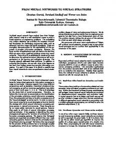
All of our neural network-based expert systems were built using the back-propagation algorithm [3], Figure 1 shows the architecture of a typical back-propagation network. The neural network in this figure has an input layer with two units, a hidden layer with three units, and an output layer with two units. Theoretically there is no limit on the number of units in any layer, nor is there limit on the number of hidden layers. For simplicity, we used one or two hidden layers for all our neural networkbased expert systems. Each layer wa,c_ fully connected to international Journal of Neural Networks, VoL 1, No. 4, October 1989
the succeeding layer, and each connection had a corresponding adjustable weight. For example, the weight of the connection between the first unit in the input layer and the second unit of the hidden layer are not labeled in Figure L During training, the weights between the last hidden layer and the output layer were adjusted to reduce the difference between the desired output and the actual output. Then, using the back-propagation algorithm, the error was transformed by the derivative of the transfer function and was back-propagated to the previous layer and the weights in front of this hidden layer were adjusted. The process of back-propagating errors continued until the input layer was reached. The back-propagation algorithm derives its name from this method of computing the error term. All the neural network-based expert systems described in this paper were developed using ANSim — Artificial Neural Systems Simulation program written by Science Applications International Corporation, although we have subsequently used Neural works by Neural Ware Inc. with similar results. We note explicitly that ANSim is a neural network simulation package, and it was never intended to be an expert system development tool. So in this paper we point out some of the problems that would have to be overcome if someone were to use it as an expert system development tool,
3.
Neural network-based expert systems
We developed two score expert systems; some with a neural network, some with traditional expert system shells. We used an IBM AT compatible computer with 4 Mb of memory. All of these expert systems were based on demonstration systems provided by the companies who market the traditional expert system shells. These demonstration systems were designed to show off the features of their products. So if the neural networkbased expert systems are better it is not because we chose straw men. These demonstration systems were developed for the shells M.I by Teknowledge Inc., VPExpert by Paperback Software International and 1st Class by Programs in Motion Inc. While M.I is a rulebased system, the other two are induction-based expert system shells, i.e. they form the rules by induction from examples given by the expert. These expert systems were small and clear enough to illustrate the advantages and disadvantages between a neural network-based expert system and shell-based expert systems. 211
Figure 1: ADAPTIVE WEIGHTS
\T DATA
INPUT DATA
OUTPUT LAYER
INPUT LAYER
HIDDEN LAYER
4.
Building neural networkbased expert systems
The first step in building a neural network-based expert system was to identify the important attributes that were necessary for solving the problem. Then all the values associated with these attributes were identified. All the possible outputs were also listed. Then several examples were listed that mapped different values of the attributes to valid results. This set of examples formed the training file for the network. The attributes and values defined the input layer of the neural network. The results formed the output layer, In this section a Wine Color Advisor that gave advice on the color of wine to choose given the type of sauce, the preferred color and the main component of the meal is shown to illustrate the steps involved in creating a neural network-based expert system. For building this system the 13 examples shown in Table 1 were used. The steps involved in creating the neural network-based Wine Color Advisor are given below. Step 1: Identify the attributes. (A) Type of sauce (B) Preferred color (C) Main component Step 2: Identify values for all the attributes. 212
(A) Type of sauce 1. Cream 2. Tomato (B) Preferred color 1. Red 2. White (C) Main component L Meat 2. Veal 3. Turkey 4. Poultry 5. Fish 6. Other Step 3: Identify the outputs.
1. Red 2. White Step 4: Make a set of examples as shown in Table 1. Step 5: Use the example to train the network. The input layer of the neural network consists of all attributes and values of the problem. Since there were three attributes, (type of sauce, preferred color, and main component) there are three rows in the input layer, International Journal of Neural Networks, Vol. 1, No. 4, October 1989
Table 1: The Wine Color Advisor Sauce Main | Advised Example Preferred Component | Color No. Color * * red 1 red * tomato * red 2 # * white white 3 * * white 4 cream * * meat red 5 * * white veal 6 * white 7 cream turkey * white 8 cream poultry * tomato 9 turkey red * tomato 10 poultry red * 11 * white fish * cream 12 white other * tomato 13 other red * means any value is acceptable for that attribute
shown in Table 2. Because the main component had six values, there are six columns in the input layer, Therefore the input layer was ( 3 x 6 ) , which means it has 3 rows having 6 units each. Because type of sauce and preferred color have only two values each, eight of these 18 input units will never be used. So the unused inputs were given values of zero. (We tried other values for unused inputs, but the large bias terms drove the net out of the central operating region, and inconsistent advice was given.) The other input units can take on values ranging from -0.5 to +0.5. Many of the values in Table 1 are represented with an * , meaning any value is acceptable. When traditional induction shells encounter such entries, they first expand the example into as many rules as there are possible values, then they try to optimize the rule base to minimize the number of rules (or whatever else they are optimizing). For example they would expand example 7 into the following two rules. 1. If type of sauce = cream and preferred color — red and main component = turkey then advised color = red. 2. If type of sauce = cream and preferred color = white and main component = turkey then advised color — white. To make the neural net behave similarly both of the inputs for preferred color must be set to true, i.e. set to +0.5. An input layer showing the 7th example from Table 1 is shown in Table 2. Here the first element in the first row takes a value +0.5 to denote that it is activated, i.e. type of sauce is Internationa! Journal of Neural Networks, Vol. 1, No, 4, October 1989
Table 2: The input layer of the neural network Attributes Sauce Preferred color Main component
1 +0.5 +0.5
2 -0.5 +0.5
3 0.0 0.0
4 0.0 0.0
5 0.0 0.0
6 0.0 0.0
-0.5
-0.5
+0.5
-0.5
-0.5
-0.5
cream. If the type of sauce were tomato, then the first element in the first row would be -0.5 and the second element of the first row would be +0.5. Since the second attribute, preferred color, is denoted by a * in the example table, both units in row 2 have values of +0.5. The third row of the input layer takes on the value for main component, for this example the third column is +0.5 representing turkey. The above describes inputs to the system during training mode. However, during a consultation inputs are treated similarly. The user can supply any number between -0.5 and +0.5 for any value of any attribute; -0.5 means false or no, +0.5 means true or yes, and 0 means unknown. Multiple values can be assigned and certainty factors can be used. Unused inputs are kept at zero. The best size, shape, and number of the hidden layers depends on the particular problem being studied and the number of examples in the training file. We expected small hidden layers would lack sufficient richness and we 213
5. Table 3: The output layer Wine Color Node Value Red -0.5 White +0,5
expected large hidden layers to exhibit increased noise because they would be under constrained. However, in experiments where we varied the size of the hidden layer form (1 x 1) (!) to (40 x 40) and computed the errors between the outputs of these neural networks and the outputs of a 1st Class-based expert system, we found no significant differences. Of course, the number of units in the hidden layer also depends upon the output layer, For an output layer of sise (n x m) the minimum number of cells in the hidden layer would be Iog2(n x m) or, depending upon the particular knowledge being encoded, perhaps Iog2(max m, n). A more detailed discussion of the hidden layer is beyond the scope of this paper. For building the neural network-based expert systems of this paper, we used either one or two square hidden layers. The hidden layer for our wine color advisor was arbitrarily chosen to be (6x6). The output layer was assize ( 2 x 1 ) because the solitary output (reeommended^colqr) had 2 values (red and white). The output vector for the above example is shown in Table 3. Now that the knowledge was formulated, it was time to train the neural network, The 13 examples of Table 1 were coded to form the input training file. This file was repeatedly presented to the network until the root mean squared error between the desired output and the actual output dropped below a preset value (usually 0.1). During the training process the network learned and adapted the values of the weights to reduce the error between the actual and desired outputs for the various combinations of inputs, The output node values of the network ranged from -0.5 to 0.5. These values indicate how certain the network was in its answer. However, because M.I, VPExpert and 1st Class used certainty factors that ranged from 0 to 100, for comparison purposes, we mapped the output node values of the neural network into a range between 0 to 100. In almost all cases the node values derived by the neural network-based expert systems were quite similar to the certainty factors derived by the traditional shellbased expert systems. We have found three exceptions to this rule. The first of these is illustrated by gradual learning. 214
Gradual learning
As more examples were added to the input training file the network changed its output node values. However, unlike induction-based expert systems where certainty factors changed abruptly, the neural network-based expert systems changed their output node values gradually, which shows gradual learning by the neural network. To demonstrate this property, the examples of Table 4 were added incrementally to the Wine Color Advisors, developed using 1st Class and the neural network. After each example was added the systems learned or induced new rules, then a consultation was run with each system with the user specifying a cream sauce, a preferred color of red, and the main component of fish. The changes in output certainty as these examples were added are shown in Table 5, Table 5 illustrates the gradual change in the output values of a neural network for each additional example that was used to teach the network. This shows that each additional example increased the knowledge represented among the connections in a neural network. This is analogous to a human gaining more experience. Here the network behaves more human like than an inductionbased expert system.
6.
Contradictory conclusion
Unlike traditional induction-based expert systems, a neural network-based expert system will not accept contradictory conclusions. To illustrate this, the original 13 example Wine Color Advisors of Table 1 were trained adding the new example shown in Table 6. Note that the new example, number 14, contradicts a previous example, number 13. From these examples, the following rules were created by the induction-based expert system shell 1st Class: 1. IF sauce = tomato THEN color = red. 2, IF sauce = tomato THEN color = white. While the induction-based shell created rules from these examples, the neural network would not. The training phase exhibited 20 cycles of transient behavior followed by steady-state behavior, where the output error oscillated between 0 and 0.5. This shows that contradictory conclusions cannot be taught to a neural network. We cannot conclude which behavior is more human like. International Journal of Neural Networks, Vol. 1, Mo. 4, October 1989
Table 4: Examples added to the wine color advisors Example | Sauce Preferred Color No. I * 14 cream * tomato 15 * tomato 16 * tomato 17 * cream 18
Main II Advised Component J[ Color meat red red veal red turkey white fish meat white
Table 5: Changes in output certainty No. of last example in training set 13 14 15 16 17 18
1st Class Certainty Factors White Red 50 50 50 50 50 50 50 50 50 50 75 25
Neural Network Node Values White Red 52 48 62 43 27 80 92 8 95 7 98 7
Table 6: Contradictory examples Example Sauce No. 13 || tomato 14 || tomato
Preferred Color * *
International Journal of Neural Networks, Vol. 1, No. 4, October 1989
Main Component other other
Advised Color red white
215
1 2 3 4 5 6 7 8 9 10 11 12 13 14 15 16 17 18 19 20
7.
Table 7: Animal Classification Examples Albatross Penguin Ostrich Zebra Giraffe Tiger • • • Coat hair * • Feeds offspring milk • * * Coat feathers • Flies * * • Lays eggs Eats meat • Pointed tooth * Extermities claws • Eye position forward * * • Extermities hooves • * Chews cud * Habitat ships * Swims • * Color black & white • • Long neck • • Long leg • Black stripes * • Dark spots Color tawny • * * Does not fly Note; The animals have the attributes indicated by the »?s
Continuous output
Traditional expert systems collect all the pertinent information, and then at the end of the consultation, give their advice. The neural network-based expert systems gave outputs continuously. As they collected more input information they gradually become more certain of an answer and they gave more certain advise. To demonstrate this, the Animal Classification Expert System based on Winston [4] was created using a neural network for identifying an animal given its features. The system was trained to classify seven different animals, Twenty different features were used to identify these animals. The examples showing the features associated with each animal are given in Table 7. The size of the input layer of this neural networkbased expert system was (20 x 1). The one hidden layer was of she (10 x 10), The output layer was ( 1 x 7 ) , It took about 30 minutes to train this network. During one consultation, when the user had a tiger in mind, the following six features were given:
* • • * *
• *
5. Black stripes 6. Tawny color To show the effect of adding .more and more features to an input vector, the network was first given one feature, then two features, then three features etc. The result of this test is shown in Table 8^ As more and more attributes were added to the input vectors, the output values of the units increased and the neural network grew more confident in its answer. It also eliminated other animals having similar features. This example demonstrated that neural network will give a good answer even with partial input.
8.
Erroneous inputs
To demonstrate the effect of erroneous data in the input, an input vector having the following attributes were given to the Animal Classification Expert System.
1. Eats meat
1. Eats meat
2. Pointed tooth
2. Extremities claws
3. Extremities claws
3, Eye position forward
4. Eye position forward
4, Black stripes
216
Cheetah
international Journal of Neural Networks, Vol. l r No. 4, October 1989
Example number 1 2 3 4 5 6 7 8 9 10 11 12 13 14 15 16 17 18 19 20 21 22 23 24 25 26 27 28 29 30 31 Legend
218
Table 9: Training Examples for Cheese Advisor Complement Cheese Cours$e Savonness Consistency A | S D M F | P S j M| F * • C&B Montrachet * C&B Montrachet * • Gorgonsola C&B * * • C&B Stilton * C&B Stilton • * C&B Kasseri * • * * Montrachet C&B * * Montrachet C&B * * * * Gorgonzola C&B * • * Stilton C&B * • Stilton C&B * • • C&B Kasseri * * * • B&F Camembert • * B&F Camembert • * • Tallegio B&F * * * * Italian Fontina B&F * * Italian Fontina B&F * * * Appenzeller B&F * * * • Brie B * * * Brie B * 9 * • Chevres B * * * • 0 Gouda B * • Gouda B * * * • Asiago B * * * * • * Brie B • * * Brie B * * * • B Chevres • • * * * B Gouda • *_ * * B Gouda * * * Asiago B * * * * Edam B * Course: A = Appetizer, S=Salad, D— Desert Savoriness: M=MiId, F=Flavorful, P=Pungent Consistency: S-Soft, M^Medium, F=Firm Complement: C&B=Crackers and Bread, B&F=Bread and Fruit, B=Bread
Internationa! Journal of Neural Networks, Vol. 1, No. 4, October 1989
9. Table 8: Neural Network Identifying a Tiger Input vector^ 1
Features activated 5
2
5,6
3
5,6,1
4 5 6
5,6,1,2 5,6,1,2,3 5,6,1,2,3,4
Output Tiger Zebra Tiger Zebra Tiger Zebra Tiger Tiger Tiger
Node value 14 14 31 8 66 .7 91 91 98
5. Tawny color 6. Coat feathers 7. Animal swims Here note that the attribute 2 was removed from the previous set and incorrect additional attributes 7 and 8 were added. In this case, even from partial information the neural network gave the correct answer, tiger, with a certainty of 87. Of course with a neural network all possible outputs have some non-sero certainty factor. For example, the last two features in the above input vector are true for a penguin. But the output node value for this animal was only 12. So the net was pretty sure that it was a tiger despite the erroneous inputs. In this example the user gave seemingly incorrect answers. It would be short sighted to say 4Well if the users cannot give the right answer, then they should not be using our system.' There are many reasons for users giving incorrect answers: new experiences, cultural differences and developmental differences. When users try different scenarios or experiment with unknown situations they often give answers the expert system was not prepared for. Also in the real world, as opposed to nice well defined model situations, complete knowledge of a situation is rare. So it is a desirable property for an expert system to allow erroneous inputs from its users. The above example shows that a neural network-based expert system can handle erroneous inputs very well. When we gave erroneous inputs to our traditional expert systems, they responded with comments like Identity of animal Is unknown5, and 'What is the value of: lays-eggs?'. Clearly the neural network-based expert system is friendlier and more human like. International Journal of Neural Networks, Vol. 1, No, 4, October 1989
Global knowledge representation
The Cheese Advisor neural network-based expert system was created to give advice about what cheese and complement to choose given the main course, preference in taste and preference in consistency of cheese. The example file, Table 9, was created from a VP-Expert demonstration expert system. An input layer of size (3 x 3), two hidden layers each of size (10 x 10), and an output layer of size (13 x 1) were used to build this network. There were 12 200 connections in this network and it took about 5 hours to train it. The information about specific objects is spread out among the connections in a neural network. So it has the natural ability to form categories and associations among these objects during the learning phase. Knowledge is represented in the form of weights throughout the network, Unlike a shell-based expert system, a neural network considers all the knowledge encompassed in its connections to come to a conclusion. This is demonstrated by a modified example from the Cheese Advisor, Two of the rules in the VP-Expert knowledge base are given below, 1. IF Complement = bread-and-fruit AND Preference = Mild OR Preference = Flavorful AND Consistency = Firm THEN The-Cheese = Italian-Fontina; 2, IF Complement = bread-and-fruit AND Preference = Pungent THEN The-Cheese = Appenzeller, Because of the OR clause in the premise of the first rule, VP-Expert actually considers the above knowledge base as 3 rules. They are: la. IF Complement = bread^andjruit AND Preference = Mild AND Consistency = Firm THEN The-Cheese = Italian-Fontina; Ib. IF Complement = bread_andJruit AND Preference = Flavorful AND Consistency = Firm THEN The-Cheese = Italian-Fontina; 2. IF Complement = bread-andJfruit AND Preference == Pungent 217
AND Consistency = Firm THEN The-Cheese = Appenzeller; When VP-Expert was asked to give advice about the type of cheese using the above rules given the following user answers, Complement = bread and fruit Preference = Flavorful with cf 50 Preference = Pungent with cf 50 Consistency = Firm two of the three rules fired and the advice was Cheese = Italian JPontina with cf 50 and Cheese = Appenzeller with cf 50, However, when the same input was given to a trained neural network, the output was, Cheese = Appenzeller with node value 89 and Cheese = ltalian_Fontina with node value 38. The VP-Expert system recommended Italian JPontina and Appenzeller with equal certainty, whereas the neural network-based expert system preferred Appenzeller with a node value of 89. Which of these is more humanlike? To answer this question, let us look at what each system is doing logically. In the VP-Expert system, two of the three rules fired: one recommended ItalianJFontina and the other said Appenzeller. The third rule failed, so VP-Expert could gather no information from that rule. Therefore VP-Expert concluded rules Ib and 2 fired, so we are about 50-50. The VP-Expert system, like most commercially available back-chaining expert system shells, uses modns ponens logic. With this type of logic we can evaluate the truth value of the conclusion, if we know the truth value of the premise. For example in this rule: IF Preference = Pungent THEN The-Cheese = Limberger If we know that the person prefers pungent cheese then we can recommend Limberger. However, with modus ponens we cannot go backward. For example, if we know that the recommended cheese is not Limberger, we know nothing about the person's preference. Furthermore, if we know that the recommendation was Limberger, we still do not know what the person's preference was because some other rule could have caused the recommendation to be Limberger. However, there are other types of logic. Some expert system shells use modus tolans logic. This is similar to if and only if (iff) rules. With modus tolans if you can prove that a conclusion is false then you know that the premise is false. For example for the rule: Internationa) Journal of Neural Networks, Vol, 1, No. 4, October 1989
IF no gas OR no spark OR starter bad THEN car will not start. We can go forward, like modus ponens: if we find out that the car has an empty gas tank we can conclude that the car will not start. However, in addition, if we find out that the car does start, then with modus tolans logic, we can conclude that the car has gas, has spark and the starter is good. We do not know what type of logic the neural network uses, but it is not modus ponens or modus tolans. The neural network saw that rule la was false. Therefore it concluded that Italian-Fontina was not to be preferred. Hence it decreased the certainty for this cheese. Its recommendation was therefore Appenzeller, The neural network, which considers all of the information stored in its connections, not just the rules that fire, gave different certainty than the traditional expert system. We have not done a post mortem dissection of the neural net, so we cannot say exactly how the output values were derived, but they seem to be more human-like. Human experts often have great difficulty providing certainty factors to the knowledge engineer. We suggest that this might be a good use of a neural network. Let it provide numbers to help human experts formulate certainty factors for their knowledge. These certainty factors could then be used in a traditional expert system. Usually neural network node values are pretty close to traditional expert system certainty factors. However, as previously stated, we have found three instances where the neural network node values behaved differently from traditional expert system certainty factors. We discussed these in the sections titled gradual learning, continuous output and global knowledge representation. Furthermore, we found that if an example in the training set exactly matched an example in the test set, then the node values of the neural network based expert systems and the certainty factors of the traditional expert systems were the same.
10.
Lesion
The knowledge is widely distributed among the connections in a neural network-based expert system. Because of this, damage to a few connections need not impair the overall performance of the network. This is possible because of the highly parallel nature of neural networks that is analogous to biological neural networks, To demonstrate the degree of robustness of a network, the neural network-based Cheese Advisor was used. The connections from input layer to the first hidden layer are 219
analogous to the axons of a sensory system of a human being. The connections between hidden layer 1 and hidden layer 2 are analogous to CNS interconnections and the connections from hidden layer 2 to the output layer are analogous to axons of the motor system. All the connections in the network had weights ranging from -5 to 5, A lesion was afflicted on a connection by setting its weight to 0, Starting at the top left hand corner of the weight matrix, the connections were systematically lesioned in increments of 5% of the total number of connections. The effect of varying degree of lesion on the connections from input layer to hidden layer is shown in Figure 2, The network was given the same 10 input vectors after each increase in the amount of lesion. Reducing the weight values to 0 for some of the 900 weights between input and the first hidden layer caused the final certainty for recommended cheese for some input vectors to decrease more than others. For example Figure 2 shows the input vectors that were affected the most, and the least, vectors 9 and 5 respectively. This is similar to what would happen as a result of a lesion in a biological system. The vectors that used the values that were lesioned out would be affected more than those that did not. Figure 3 shows the effects pf lesions in between the two hidden layers. As expected, different input vectors are now rnbs^t and least affected. Vectors 3 and 2 respectively. More importantly we see that the effects are distributed more evenly than in Figure 2, The most affected vector only drops to 73 (versus 70 for Figure 2) and the least affected vector drops all the way down to 85 (versus 93 for Figure 2), These effects are also similar to lesions in biological systems. Sensory lesions affect one aspect more than others. But CNS lesions do not have such precise effects. Effects of CNS lesions are more general or diffused. In traditional expert systems, to make deficits similar to the sensory lesions, we could remove a few questions. If an input vector needed to invoke fliat question, then a deficit would be noticed. If it did not need that question no deficit would be seen. This is similar to neural network performance except that the degradation of the neural network is gradual and that of the traditional expert system is abrupt. Similarly, lesions in the motor output of a neural network would be akin to erasing the output advice of a traditional expert system. However, there seems to be no analog of CNS lesions in traditional expert systems. There are no rules that you can erase that will affect, all input vectors marginally, without causing major effects in some. 220
11.
Sparse input layer
The Flower Planning Guide was an expert system created using a neural network to give suggestions on the flowers for a garden based on: color, season, average height, flowering time and shade tolerance. The examples used to train this system are shown in Table 10. This table has five attributes, and one of them, average height, has 33 possible values, ranging from 4 to 36 inches. Therefore, we tried to create a network with an input layer of size (33 x 5). Experience seems to indicate that the smallest edge of the hidden layer should be at least as big as the biggest edge of the input layer. This would have required an hidden layer of 33 by 33. The output layer has to be (1 X 25) because 25 different flowers are specified. Such a neural net would have required 206910 connections, and with only 4 Mb of RAM we were limited to 60000 connections. Therefore, we restricted the values for average height to be even numbers, and an input layer of size (17 x 5) was built. The hidden layer was of size (17 x 17) and the output layer was (1 x 25). There were 31 790 connections in this network. This expert system correctly learned all 31 examples. However, after 336 passes through the input training file, which took 23 hours, the total root mean squared (rms) error was still decreasing. We believe this long learning time was caused byjthe sparse use of the input layer. In this network only ^the attribute average height used all the 17 units in its low to encode information about different flowers. The rest of the attributes all had less than six values. So the full input layer was not completely used by these attributes. To eliminate the effect of sparse input layer, we made another network in which the different attributes formed a linear input vector. There were 30 units representing the total number of values of all attributes. There were two values for life span, five values for color, three for flower season, 17 for average height, and three for shade tolerance. So the input layer for the network was of sige (30 x 1), the hidden layer was (17 x 17) and the outpuo layer was (25 x 1). However, this network got caught in a local minimum during training; the total rms error quickly dropped to 0,19, but then it stayed there forever (actually we stopped it after 18 hours). We used several different techniques to shake networks out of local minima. 1. We added input noise that decayed away after a few cycles, and then we started retraining, 2. We damaged some weights, and then started retraining, 3. We damaged weights and added input noise, and then started retraining. international Journal of Neural Networks, Vol, 1, No. 4, October 1989
Table 10: Flower planning guide examples Flower Average Sun or Type Height Shade (inches) Berginia 1 Perennial Shade 12 Red Spring Perennial Shade Blueberry 2 Blue 12 Spring Bleed-Heart Shade Perennial 12 3 Summer Red * Viola Part-Shade 4 Perennial Summer 6 Annual White Candytuft Spring Sun 5 6 PartJShade Ajuga Perennial Violet Spring 6 6 Honesty Annual 7 Violet 24 Part-Shade Spring * Delphinium Perennial 30 Sun 8 Summer 12 Lavender Sun 9 Perennial Violet Summer * Perennial Summer 30 Dalily 10 Red * Dalily Perennial Yellow Summer 30 11 Alyssum White Summer Sun Annual 4 12 Peony Perennial Red Summer Sun 13 30 Peony Perennial White Summer 14 Sun 30 Peony Yellow 24 Summer Sun Perennial 15 Dianthus Perennial Summer Sun 16 Red 8 EngJDaisy Annual 17 White Summer 6 Sun Perennial Yarrow Yellow Summer Sun 30 18 Gazania Annual 19 Yellow Summer 10 Sun Columbine * Perennial Summer 24 Sun 20 Part-Shade Columbine * Summer 24 Perennial 21 Blue Sun Japan Jris Perennial Summer 22 30 JapanJris Perennial White Summer Sun 23 30 Blue Shade Lungwort Perennial Spring 24 10 Perennial Yellow Summer BLEyed-Su 30 Sun 25 Perennial * 26 Autumn 16 Sun Hardy-Aster Part-Shade Red Cranesbill Perennial Summer 18 27 Part-Shade Perennial Blue 30 Lobelia Autumn 28 Part-Shade Lobelia Perennial Red Autumn 20 29 Perennial White Autumn Part-Shade Jap_Anemon 36 3.0 Poppy Perennial Red 31 Summer 30 Sun Note: When 1st Class encounters an asterisk (*) it assumes any value is legal. When the neural network is trained, an item with an asterisk is given a node value of zero. Example number
Life Span
Color
Flower Season
International Journal of Neural Networks, Vol. 1, No. 4, October 1989
221
OUTPUT VALUES
OUTPUTVALUES oO-J
CO
m
a 1 W ffl
S-"
to I-H
3
I O J3-
O-
1 I I
$ 0 4i
O
4. We set the learning rate for the input-to-hidden layer higher than the hidden-to-output layer and trained the network until a plateau was reached, then we lowered the learning rate and proceeded to retrain. Often these techniques had to be repeated five or six times. When we used these techniques on the (30 x 1) input vector network, it learned 25 of the 31 examples and the rms error dropped to 0.09, Therefore, we conclude that the linear input array is satisfactory, but it is not superior to the (17 x 5) input layer. Perhaps the problem was that the edge of the input layer was larger than that of the hidden layer. In summary, the network with the (17x5) input layer was convenient, because each attribute had its own row. This network worked well but wasted a lot of connections with unused inputs. In an attempt to ameliorate this problem we changed the input layer to (30 x 1), but this network did not perform as well as the network with the (17x 5) input layer. It seems that we could now try several other configurations for the input layer, e.g. (10 x 3) or (6 x 5). However, rather than discuss these other configurations, let us now look at a different way of encoding the average height information. Instead of binning the average height data so that only one of the 17 input units can be active at a time, let us encode the average height as a binary number so that from zero to six input units will be active. In this representation the binary number 0 is encoded with -0.5 and the binary 1 is encoded with + 0.5. Table 11 shows this encoding for the Viola, example 4 of Table 10. The average height for this example is six inches or 000110 binary, as shown in the fourth row of the following table. When this binary coding was applied to the network with a (17 x 5) input layer, a network with a (6 x 5) input layer illustrated in Table 11 was produced. This network also had problems getting stuck in local minima during training. It learned only 25 of the 31 examples. For completeness we also Lried the other combination; we applied the binary coding to the (30 x 1) input layer network to produce a network with a (19x 1) input layer. It also got stuck in local minima and it learned only 22 of the 31 examples. Therefore we have shown that the shape of the input layer is important. We have not seen similar reports in the literature. So, summarizing this section, we can say that the network with a (17 x 5) input layer was the best. Networks with linear input layers or binary coding did not work as well, unfortunately we cannot explain why, However, the techniques of using linear input layers and binary coding worked well for our smaller Wine Color Advisor. As a second summarizing point we note that our previous sections showed that a neural network may be an International Journal of Neural Networks, Vol. 1, No. 4, October 1989
Table 11: Input layer with binary coding for height Values 3 4 0.0 0.0
5 0.0
6 0.0
+0.5
+0.5
+0.5
0.0
+0.5
-0.5
0.0
0.0
0.0
-0,5
-0.5
-0.5
+0.5
+0.5
-0.5
-0,5
+0.5
-0.5
0.0
0.0
0.0
Attributes Life Span
+0.5
2 -0.5
Color
+0.5
+0.5
Flower Season
-0.5
Average Height Shade Tolerance
1
appropriate tool for problems with discrete values for the attributes, However, this flower selection system illustrates that they may be inappropriate for problems where the attributes have a continuous distribution of values, such as weight, height and temperature, unless these attributes can be binned into a small number of ranges.
12.
Time for training
The expert systems we created using a neural network required 15 minutes to 23 hours for training. As the number of units in the network increased, the time for training also increased. This is due to the fact that all the networks were simulated in software and trained on a sequential machine. The inherent property of parallelism in neural networks cannot be fully exploited if they are trained on this type of machine. This is a disadvantage of a neural network-based expert system if created in a sequential machine. The induction-based systems took only a few seconds to form the rule base from the examples. However, hardware implementation of neural networks which will consist of highly interconnected electronic components can be used to train it much faster. In this case, neural network-based expert systems can be used for many real time applications. 223
13.
Comparison of expert systern tools
Neural networks use a different technology for building expert systems than other expert svstem shells. When using a neural network-based expert system the domain need not be as well understood as when using traditional expert system shells, Experts are not required to detail how they arrive at a solution, since the system learns this on a stimulus/response basis and self configures into a structure capable of solving the problem. The most significant advantage of using this type of expert system is that it requires no explicit algorithms or software. Hardware implementation of this technology will result in more speed, reliability (robustness) and realtime adaptivity. However, there is no formal method to validate the results of this system. This is one major disadvantage. Another problem with neural network-based expert systems is that the networks are not adaptive to growth in problem size. Also the number of connections and thus memory and time requirements tend to grow exponentially (especially in a sequential computer). In this study we made expert systems using four commercial software packages: (1) M.I by Teknowledge, (2) VP-Expert by Paperback Software International, (3) 1st Class by Programs in Motion, and (4) AN Sim by Science Applications International Corporation. Once again we explicitly note that ANSim was not designed to make expert systems so some of these comparisons may be unfair. To make a pinpoint comparison between these four tools, we made the same expert system using all four tools. We chose to do this with the Wine Color Advisor. The results are shown in Table 12.
14.
Putting it all together
In general neural networks were not designed to make expert systems. However, we have shown that they can be used to successfully create expert systems. We have shown several examples in this paper and we know of one commercial system [5]. Although the expert systems shown in this paper had only 13 to 31 examples, in general neural networks work better if they have far more examples. To make the expert systems we had to overcome some obstacles. For example, in this paper we showed how we treated unknown and unused inputs. We also compared and contrasted neural network-based expert systems to expert systems made with traditional shells. A neural network-based approach may give us a system that essentially builds its rule base from examples given by the human expert. But unlike conventional expert systems, 224
this can be achieved with minimum of outside intervention, so that over time the network gradually takes over the task of the human expert, However, we caution that the rules and generalizations made by the neural networks are not open to examination, although tools for examining such networks will surely be forthcoming. Even if some of the connections are damaged the neural network will still give a reasonable answer. This is not the case with the traditional expert system shells where if some of the rules were taken out of the knowledge base, the system failed. They may not even give an answer at all. The neural networks behaves much better with erroneous or incomplete input than a shell-based expert system because it uses all the knowledge encompassed in its connections. In fact, neural networks-based expert systems can be used to help suggest certainty factors to humans. A neural network-based expert system will increase the knowledge represented in its connections over time by learning from more examples. However, we again caution that we could not determine how the node values were derived by the neural network.
15 *
Acknowledgement
Research of this paper was partially supported by Grant Nr. AFOSR-88-0076 from the Air Force Office of Scientific Research.
16.
References
[1] J.J. Hopfield and D.W, Tank, 'Computing with neural circuits: a model7, Science, 233, 1986, pp. 625 -633. [2] M. Caudill, 'Neural networks primer, part IV, AI Expert, 38, 1988, pp. 61 - 66. [3] D.E. Rumelhart, G.E. Hinton and R.J. Williams, 'Learning representations by back-propagating errors', Nature, 323, 1986, pp. 533 - 536. [4] P.H. Winston, Artificial Intelligence, AddisonWesley, 1977. [5] E. Collins, S. Ghosh and C. Scofield, 'Risk Analysis', in DARPA Neural Network Study, 1988, Fairfax VA, Armed Forces Communications and Electronics Association (AFCEA), pp. 429 - 443.
International Journal of Neural Networks, Vol. 1, No. 4, October 1989
Table 12; Comparison of Expert System Tools Creates expert system from examples In example file * means Access to dBase, Lotus 1-2-3 etc. Use any ASCII editor Multi-valued expressions User can respond unknown cf supplied by user cf in premises cf in conclusions Variables Single valued cutoff Backward chaining Forward chaining User interface Explanation facility Intermediate values
M.I no
VP-Expert yes
Ist-class yes
ANSim
NA
Any
Any
any
hard
very easy
easy
yes
yes yes
yes yes
no yes, with ICO
yes yes
yes
only if written in rules yes yes yes no no yes a little poor yes yes, by linking knowledge bases
yes, in match mode no no yes yes yes yes somewhat super yes yes, by linking knowledge bases
yes
yes yes yes yes yes yes yes good yes yes
yes
yes yes yes NA no no yes difficult no
yes, by linking different networks yes super super yes
no no no Gradual learning poor Continuous output good okay poor Fault tolerance good okay no no no Global Knowledge representation accepts no accepts accepts Contradictory conclusions significant Effect of lesions significant significant small Time to make knowl1 hour 1/2 hour 1/2 hour 1/2 hour edge base Time to induce rules 5 seconds 5 seconds 1 hour NA NA - means this item does not apply to expert systems created using this technology
International Journal of Neural Networks, Vol. 1, No, 4, October 1989
|
225
The authors A. Terry Bahill A. Terry Bahill was born in Washington, PA, on January 31, 1946. He received a BS in electrical engineering from the University of Arizona, Tucson, in 1967, an MS in electrical engineering from San Jose State University, in 1970, and a PhD in electrical engineering and computer science from the University of California, Berkeley, in 1975. Since 1984 he has been a Professor of Systems and industrial Engineering at the University of Arizona in Tucson. His research interests include systems engineering theory, modelling physiological systems, head and eye coordination of baseball players, and expert systems. Dr. Bahill is a member of the following IEEE societies: Systems, Man and Cybernetics; Engineering in Medicine and Biology; Computer; Automatic Controls and Professional Communications.
226
Rafeck Kottai Rafeck Kottai was born in India on 28 May, 1964. He received a BTech degree from the Government Engineering College, Trichur, India, in 1986, and an MS in systems engineering from the University of Arizona, Tucson, in 1988, He is now working as a systems engineer in San Francisco, CA.
International Journal of Neural Networks, Vol. 1, No. 4, October 1989