Hindawi Mathematical Problems in Engineering Volume 2018, Article ID 7387650, 13 pages https://doi.org/10.1155/2018/7387650
Research Article Fuzzy Weighted Least Squares Support Vector Regression with Data Reduction for Nonlinear System Modeling Xiaoyong Liu
,1 Aijia Ouyang ,2 and Zhonghua Yun
3
1
College of Engineering, Zunyi Normal University, Zunyi 563006, China School of Information Engineering, Zunyi Normal University, Zunyi 563006, China 3 School of Instrument Science and Engineering, Southeast University, Nanjing 210096, China 2
Correspondence should be addressed to Aijia Ouyang;
[email protected] Received 21 June 2018; Accepted 29 November 2018; Published 10 December 2018 Academic Editor: Piotr Jędrzejowicz Copyright © 2018 Xiaoyong Liu et al. This is an open access article distributed under the Creative Commons Attribution License, which permits unrestricted use, distribution, and reproduction in any medium, provided the original work is properly cited. This paper proposes a fuzzy weighted least squares support vector regression (FW-LSSVR) with data reduction for nonlinear system modeling based only on the measured data. The proposed method combines the advantages of data reduction with some ideas of fuzzy weighted mechanism. It not only possesses the capability of illuminating local characteristic of the modeled plant but also can deal with the problem of boundary effects resulted from local LSSVR method when the modeled data is at the boundary of whole data subset. Furthermore, in comparison of the SVR, the proposed method only utilizes fewer hyperparameters to construct model, and the overlap factor 𝜆 can be chosen in relatively smaller value than SVR to further reduce more computational time. First of all, distilling the original input space into several regions with fuzzy partition by applying Gustafson-Kessel clustering algorithm (GKCA) is a foundation for data reduction and the overlap factor is introduced to reduce the size of subsets. Following that, those subset regression models (SRMs) which can be simultaneously solved by LSSVR are integrated into an overall output of the estimated nonlinear system by fuzzy weighted. Finally, the proposed method is demonstrated by experimental analysis and compared with local LSSVR, weighted SVR, and global LSSVR methods by using the index of computational time and root-meansquare error (RMSE).
1. Introduction It is well known that, in a large number of applications such as advanced control, process simulation, fault detection, or other research areas, a significant problem is to construct mathematical model of estimated system only based on its measured data. Some major theories or methods on identifying nonlinear system have been independently developed in various research field including fuzzy system [1], neural networks [2], and other approach [3]. However, LSSVR method [4], like SVR [5], also adopts the structural risk minimization and has the better equilibrium between sparsity and modeling accuracy. Furthermore, LSSVR, by substituting a set of equality conditions for complex inequalities ones, translates complex quadratic optimization as a simple linear programming, which is greatly relieve computational load. In literature [6], the power of generalization for LSSVR is no worse than that SVR.
Therefore, the LSSVR has been attracting extensive attentions and has obtained successful application like time series prediction [7, 8], subspace identification [9, 10], signal processing [11, 12], and other applications [13, 14] during the past few years. In spite of the LSSVR approach, referred to as the global LSSVR (G-LSSVR) approach, has become an effective tool in various applications, and can identify an estimated model whose modeling accuracy is guaranteed by obtaining an appropriate mathematical model [15] and a proper hyperparameter set which usually consists of the two variables: the kernel width (𝜎) and the penalty factor (𝛾). Generally, it is an insignificant for global-LSSVR to derive a well local behavior. We discovers in literature [15, 16] that GLSSVR has also some defective in illuminating local behavior. Recently, local modeling approaches, as an alternative efficient algorithm, because of their superiorities to identify various areas of estimated nonlinear system, seem desirable. In the literature [17], a local fusion modeling method based
2 on LSSVR and nerofuzzy has been proposed. It employs LSSVR and a learning method named as layering two kind of problem to construct each local model. In the literature [18], it adopts another approach which makes use of interest training point to identify local model instead of all points and by applying vector-norm distance [19] to search for 𝐾 nearest points. To seek a set of optimal data points, a Euclidian distance measurement method [20, 21] is proposed and the local model is set up according to these neighboring points. From the pointview of capturing the local behavior, our aims are to construct their connection between some models and the localized support vector regression (LSVR) method [22] has been proposed. Considering the much more computational time of G-LSSVR, a local grey SVR [23] is developed to speed up the calculational time. Further, by introducing regularization, a general local and global learning framework [24] formulates multiple classifier in each data of neighbours. Nevertheless, the local modeling approaches or localLSSVR have more superiorities in identifying local characteristics than that approaches such as global-SVR or LSSVR; it is still unsatisfactory in modeling global capability. First, due to the different criterion to select 𝐾 nearest neighbor training data in subsets, the better performance for localLSSVR is not derived when those training data are at the boundary area. Second, because the number of constructing all local models is equal to the size of testing set, the local LSSVR approach generally leads to a heavy computation load [16]. Third, it generates boundary effects resulting from local LSSVR method when the modeled data is at the boundary of whole data subset. Based on the above consideration, our aims present a FW-LSSVR method for nonlinear system modeling based only on the obtained measure data. The paper integrates the superiorities of GKCA, weighted average mechanism, and some ideas from LSSVR. First of all, distilling the original input space into several regions with fuzzy partition by applying GKCA is a foundation for data reduction. Following that, those subset regression models (SRMs) which can be simultaneously solved by LSSVR are integrated into an overall output of the estimated nonlinear system by fuzzy weighted. The proposed method not only possesses the capability of illuminating local characteristic of the estimated models but also can deal with the problem of boundary effects resulted from local LSSVR method. Furthermore, in comparison of the support vector regression (SVR), the proposed method only utilizes fewer hyperparameters to construct model, and the overlap factor 𝜆 is chosen in relatively smaller value than SVR to further reduce more computational time. Finally, experimental analysis demonstrates that our approach not only overcomes the disadvantages of local LSSVR, weighted SVR, and global LSSVR methods in the process of modeling nonlinear system but also has better root-mean-square error (RMSE) performance and needs less computational time. The paper is organised as follows: brief descriptions for LSSVR and GKCA in Section 2 are firstly given, the proposed method is introduced in detail in Sections 3 and 4 shows several examples for demonstrating our approach, and Section 5 summarizes the whole paper.
Mathematical Problems in Engineering
2. Preliminaries 2.1. Least Squares Support Vector Regression. It has been shown that the generalization performance for LSSVR presented by [25] is comparable to that of the SVR through a meticulous empirical study [6]. Next, we will concisely introduce LSSVR with the following training points, where 𝑥𝑘 ∈ 𝑅𝑛 is the input pattern and 𝑦𝑘 is the corresponding target. (𝑥1 , 𝑦1 ) , . . . , (𝑥𝑁, 𝑦𝑁)
(1)
The LSSVR can be represented for a test input 𝑥 as 𝑁
𝑓 (𝑥) = ∑ 𝛼𝑘 𝐾 (𝑥, 𝑥𝑘 ) + 𝑏
(2)
𝑘=1
Because of adopting the Gaussian kernel width, kernel function 𝐾(𝑥, 𝑥𝑘 ) in (2) can further be rewritten as 2 − 𝑥 − 𝑥𝑘 𝑓 (𝑥) = ∑ 𝛼𝑘 exp ( )+𝑏 2𝜎2 𝑘=1 𝑁
(3)
where support-value-vector 𝛼 = [𝛼1 , 𝛼2 , . . . , 𝛼𝑁]𝑇 and bias 𝑏 are solved by formulating the following optimization [25]: min2
𝑤,𝑏,𝜉𝑘
𝑠.𝑡.
𝚥1 (𝑤, 𝑏, 𝜉) =
1𝑁 1 𝑇 𝑤 𝑤 + 𝛾 ∑ 𝜉𝑘2 2 2 𝑘=1
𝑦𝑘 = 𝑤𝑇 Φ (𝑥𝑘 ) + 𝑏 + 𝜉𝑘 ,
(4)
𝑘 = 1, 2, . . . , 𝑁.
where Φ(⋅) represents a feature mapping which nonlinear space is transformed to a high-dimensional linear space and parameter 𝛾 ∈ R+ is regularization constant which governs the relative importance between the data fitting and the smoothness of the solution. Using Lagrange multiplier method for (4) gives rise to an unconstrained optimization problem: 𝐿 1 (𝑤, 𝑏, 𝜉; 𝛼) = 𝚥1 (𝑤, 𝑏, 𝜉) 𝑁
− ∑ 𝛼𝑘 (𝑤𝑇 Φ (𝑥𝑘 ) + 𝑏 + 𝜉𝑘 − 𝑦𝑘 )
(5)
𝑘=1
In terms of the KKT condition, one derives 𝑁 𝜕𝐿 1 = 0 → 𝑤 = ∑ 𝛼𝑘 Φ (𝑥𝑘 ) 𝜕𝑤 𝑘=1 𝑁 𝜕𝐿 1 = 0 → ∑ 𝛼𝑘 = 0 𝜕𝑏 𝑘=1
(6)
𝜕𝐿 1 = 0 → 𝛼𝑘 = 𝛾𝜉𝑘 𝜕𝜉𝑘 𝜕𝐿 1 = 0 → (𝑤𝑇Φ (𝑥𝑘 ) + 𝑏) − 𝑦𝑘 + 𝜉𝑘 = 0, 𝜕𝛼𝑘 𝑘 = 1, 2, . . . , 𝑁
Mathematical Problems in Engineering
3
Consequently, learning process of LSSVR corresponding to (5) is implemented by solving (
0 𝑏 1𝑇𝑁 0 )( ) = ( ) −1 1𝑁 Ω + 𝛾 𝐼𝑁 𝛼 𝑦 𝑇
(7) 𝑇
where 𝑦 = [𝑦1 , 𝑦2 , . . . , 𝑦𝑁] , 1𝑁 = [1, 1, . . . , 1] , Ω𝑖𝑗 = 𝐾(𝑥𝑖 , 𝑥𝑗 ) = Φ(𝑥𝑖 )𝑇Φ(𝑥𝑗 ), and ∀𝑖, 𝑗 = 1, 2, . . . , 𝑁, with 𝐾(⋅, ⋅) a positive-definitive Mercer kernel function meeting the Merer’s theorem. 2.2. Gustafson-Kessel Clustering Algorithm. Clustering analysis plays an important role in classification and regression problem. In order to study some important characteristics of complex system, it is crucial for researchers to decompose an original data set into several subsets which is well reflect a system’s behavior. Especially, GKCA [26] used for extracting various clustering center in different shape and direction for a larger data set [27] and is superior to conventional FCM. GKCA can be achieved by minimizing the following objective function: 𝑅 𝑁
𝑇
𝑚 𝐽 = ∑ ∑𝜇𝑖𝑘 (𝑥𝑖 − ^𝑘 ) 𝑀𝑘 (𝑥𝑖 − ^𝑘 )
(8)
𝑘=1𝑖=1
𝑅
∑ 𝜇𝑖𝑘 = 1,
𝑖 = 1, 2, . . . , 𝑁
(9)
𝑘=1
𝜇𝑖𝑘 is a component from fuzzy matrix 𝑈, 𝑀𝑘 is defined by (12), 𝑅 describes the number of clustering center ^𝑘 , and it needs to be predefined. In a nutshell, GKCA can be boiled down to the following steps: (1) calculating the cluster centers 𝑚
^𝑘(𝑙)
=
(𝑙−1) ∑𝑁 𝑖=1 (𝜇𝑖𝑘 ) 𝑥𝑖 (𝑙−1) ∑𝑁 𝑖=1 (𝜇𝑖𝑘 )
𝑚
,
1≤𝑘≤𝑅
(10)
where 𝑙 denotes iteration number and 𝑁 is the number of all data points. (2) computing 𝐹𝑘 according to the definition of covariance 𝑚
𝐹𝑘 =
(𝑙−1) (𝑙) (𝑙) ∑𝑁 𝑖=1 (𝜇𝑖𝑘 ) (𝑥𝑖 − ^𝑘 ) (𝑥𝑖 − ^𝑘 ) 𝑚
(𝑙−1) ∑𝑁 𝑖=1 (𝜇𝑖𝑘 )
𝑇
,
(11) 1≤𝑘≤𝑅
(3) computing the distance 𝑀𝑘 = det (𝐹𝑘 )
1/𝑛
(𝐹𝑘 )
−1
𝑇
𝑑2𝑖𝑘𝑀𝑘 = (𝑥𝑖 − ^𝑘(𝑙) ) 𝑀𝑘 (𝑥𝑖 − ^𝑘(𝑙) )
(12)
1 ∑𝑅𝑗=1 (𝑑𝑖𝑘𝑀𝑘 /𝑑𝑗𝑘𝑀𝑘 )
, 2/(𝑚−1) (13) 1 ≤ 𝑖 ≤ 𝑁, 1 ≤ 𝑘 ≤ 𝑅
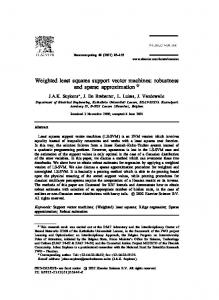
3. Fuzzy Weighted Least Squares Support Vector Regression The paper develops a new method combining respective advantages both global and local learning method to formulate overall framework. The procedures of the proposed FWLSSVR approach are depicted by Figure 1. 3.1. Constructing Fuzzy Weighted with Triangle Membership Functions. Applications of fuzzy concepts were early devel̃ can be oped by Zadeh [28]. A triangular fuzzy number 𝐴 𝐿 𝑀 𝑅 𝐿 parametrized by a triplet (𝑎 , 𝑎 , 𝑎 ), where 𝑎 and 𝑎𝑅 denote the left and right bounds, respectively, and 𝑎𝑀 represents the ̃ The membership function of the triangular fuzzy mode of 𝐴. ̃ is defined by number 𝐴 𝑢 < 𝑎𝐿 {0, { { { { { (𝑢 − 𝑎𝐿 ) { { { , 𝑎𝐿 ≤ 𝑢 ≤ 𝑎𝑀 { 𝑀 𝐿) (𝑎 − 𝑎 𝜇𝐴̃ (𝑢) = { { (𝑎𝑅 − 𝑢) { { { { , 𝑎𝑀 ≤ 𝑢 ≤ 𝑎𝑅 { 𝑅 𝑀 { { { (𝑎 − 𝑎 ) 𝑢 ≥ 𝑎𝑅 {0,
(14)
̃ in the universe of discourse The 𝛼-cut 𝐴 𝛼 of the fuzzy set 𝐴 𝑈 is defined by 𝐴 𝛼 = {𝑢𝑖 | 𝜇𝐴̃ (𝑢𝑖 ) ≥ 𝛼, 𝑢𝑖 ∈ 𝑈}
(15)
where 𝛼 ∈ [0, 1]. In generally, fuzzy partition is implemented by some clustering methods and GKCA [26] is common used to decompose the original data set. It discovers that GKCA is superior to that of FCM(fuzzy c-means) and subtractive clustering. GKCA extended the standard FCM algorithms by adopting a flexible distance measure that is calculated using covariance matrices as exhibited in (11). Meanwhile, various difformities and orientation in original data set are detected by GKCA. In this paper, GKCA is used, in which it is based on the minimization of (8). As stated in Section 2.2, the iteration is to be stopped when the termination criterion is satisfied, namely, ‖𝑈(𝑙) − 𝑈(𝑙−1) ‖ < 𝛿, and an appropriate fuzzy membership matrices is obtained finally. Following that, the cluster centers ]𝑘𝑗 and spread widthes 𝜌𝑘𝑗 are calculated, respectively, as [29] ]𝑘𝑗 =
(4) revising the components 𝜇𝑖𝑘 of fuzzy matrix (𝑙) = 𝜇𝑖𝑘
The iteration stops when the difference between the fuzzy partition matrices 𝑈(𝑙) and 𝑈(𝑙−1) in the following iterations are lower than 𝛿.
𝜌𝑘𝑗 =
∑𝑁 𝑖=1 𝑥𝑖𝑗 𝑢𝑘𝑖 ∑𝑁 𝑖=1 𝑢𝑘𝑖
2 𝑥𝑖𝑗 − ]𝑘𝑗 ∑𝑁 𝑖=1 𝑢𝑘𝑖 ∑𝑁 𝑖=1 𝑢𝑘𝑖
(16)
(17)
𝑖 = 1, 2, . . . , 𝑁; 𝑘 = 1, 2, . . . , 𝑅; 𝑗 = 1, 2, . . . , 𝑛 (18)
4
Mathematical Problems in Engineering
Start
Set the number of clusters R
Applying GKCA to original training data
Training subset 1 1
Training subset 2 2
Computing the cluster center and the spread width for each of training subsets
Triangle membership function
New training subset 1
Training subset R R
Setting the overlap factor to reacquire new training subsets
New training subset 2
LSSVR SRM-1
weighted values
New training subset R
LSSVR
LSSVR SRM-R
SRM-2
Weighted Average mechanism
Output of the estimated model
Figure 1: An illustration for the proposed FWA-LSSVR approach.
where 𝑁 is the number of training data, 𝑅 is the number of clusters, 𝑢𝑖𝑘 is the degree of membership of 𝑥𝑖 in the cluster 𝑘, 𝑥𝑖 is the 𝑖th training data, 𝑛 is a feature dimensionality, and ‖ ∗ ‖ measures the distance between two vectors. From (16) and (17), the weighted values can be calculated by applying triangle membership functions. In order to derive the weighted values, triangle membership function 𝜇𝑘 (𝑥𝑖𝑗 ) is constructed as follows according to (14): 𝜇𝑘 (𝑥𝑖𝑗 ) 0 { { { { { { 𝑥𝑖𝑗 − (]𝑘𝑗 − 𝜆 ⋅ 𝜎𝑘𝑗 ) { { { { { { { { ]𝑘𝑗 − (]𝑘𝑗 − 𝜆 ⋅ 𝜎𝑘𝑗 ) = { ]𝑘𝑗 + 𝜆 ⋅ 𝜎𝑘𝑗 − 𝑥𝑖𝑗 { { { { { { (]𝑘𝑗 + 𝜆 ⋅ 𝜎𝑘𝑗 ) − ]𝑘𝑗 { { { 0 { { { { {1
]𝑘𝑗 < 𝑥𝑖𝑗 < ]𝑘𝑗 + 𝜆 ⋅ 𝜎𝑘𝑗 𝑥𝑖𝑗 ≥ ]𝑘𝑗 + 𝜆 ⋅ 𝜎𝑘𝑗 𝑥𝑖𝑗 = ]𝑘𝑗
𝑛
𝛽𝑘 (𝑥𝑖 ) = 𝜇𝑘 (𝑥𝑖1 ) ⋅ 𝜇𝑘 (𝑥𝑖2 ) ⋅ ⋅ ⋅ 𝜇𝑘 (𝑥𝑖𝑛 ) = ∏𝜇𝑘 (𝑥𝑖𝑗 ) 𝑗=1
(20)
𝑖 = 1, 2, . . . , 𝑁; 𝑗 = 1, 2, . . . , 𝑛 𝑘 = 1, 2, . . . , 𝑅 By the normalized firing level of the 𝑘th fuzzy sets, weighted values 𝜔𝑘 (𝑥𝑖 ) is finally calculated as
𝑥𝑖𝑗 ≤ ]𝑘𝑗 − 𝜆 ⋅ 𝜎𝑘𝑗 ]𝑘𝑗 − 𝜆 ⋅ 𝜎𝑘𝑗 < 𝑥𝑖𝑗 < ]𝑘𝑗
̃ the overlap factor Instead of (15), 𝛼-cut 𝐴 𝛼 of the fuzzy set 𝐴, 𝜆 is introduced into triangle membership functions to more readily dominate the size of original data subsets, and the degree of fulfilment 𝛽𝑘 (𝑥𝑖 ) is calculated in terms of
𝜔𝑘 (𝑥) = (19)
𝛽𝑘 (𝑥) 𝑅 ∑𝑘=1 𝛽𝑘 (𝑥)
(21)
In some applications [30], Gaussian membership function is adopted 2 𝜇𝑘 (𝑥𝑖𝑗 ) = exp (−𝜃 𝑥𝑖𝑗 − 𝜄𝑘𝑗 ) (22) 𝑖 = 1, 2, . . . , 𝑁; 𝑘 = 1, 2, . . . , 𝑅; 𝑗 = 1, 2, . . . , 𝑛
Mathematical Problems in Engineering
5
where 𝜃 = 4/𝜏2 and 𝜏 ≥ 0 describing the width of the Gaussian fuzzy function, which is usually chosen as a interval [0.3, 0.5]. 3.2. FW-LSSVR with Data Reduction. Takagi-Sugeno fuzzy models [31] have recently become a powerful practical instrument in identifying the complex system. Based on the fuzzy partition, nonlinear description of estimated system can well be expanded into several simple linear descriptions by applying rules of if-then 𝑅𝑖 : 𝐼𝑓 𝑥𝑖1 𝑖𝑠 𝜇𝑖1 (𝑥𝑖1 ) 𝑎𝑛𝑑 ⋅ ⋅ ⋅ 𝑎𝑛𝑑 𝑥𝑖𝑛 𝑖𝑠 𝜇𝑖𝑛 (𝑥𝑖𝑛 ) 𝑡ℎ𝑒𝑛 𝑦𝑖 = 𝑎𝑇𝑖 𝑥 + 𝑏𝑖
𝑖 = 1, 2, . . . , 𝑅
(23)
Here 𝜇𝑖1 , 𝜇𝑖2 , . . ., 𝜇𝑖𝑛 are the fuzzy membership function of 𝑥𝑛 , 𝑦𝑛 is corresponding output, and 𝑎 and 𝑏 are defined as consequent parameter. There are the fuzzy sets assigned to corresponding input variables, variable 𝑦𝑖 represents the value of the 𝑖th rule output, and 𝑎𝑖 and 𝑏𝑖 are parameters of the consequent function. For the input 𝑥, fuzzy weighted output 𝑓̂ can be summarized as 𝑅
𝑓̂ (𝑥) = ∑𝜔𝑖 (𝑥) (𝑎𝑇𝑖 𝑥 + 𝑏𝑖 )
(24)
𝑖=1
where 𝜔𝑖 (𝑥) represents the normalized firing strength of the 𝑖th rule for the 𝑘th sample and is computed by (20) and (21). Next, substituting linearizing around a point, the proposed method make use of the subset regression models (SRMs) which are simultaneously solved by LSSVR in each fuzzy partition area. Firstly, the original input data set is divided into several subsets with fuzzy partition. In each region, SRM is independently trained by LSSVR. Based on the obtained centers ]𝑘𝑗 and the spread width 𝜌𝑘𝑗 from (16) and (17), the old data set is once again decomposed into a new one △𝑘 by introducing the overlap factor 𝜆 to reduce the size of original subsets. We can perform the partition by the following pseudo code: 𝑓𝑜𝑟 𝑘 = 1 : 𝑅
𝑒𝑛𝑑 𝑒𝑛𝑑 (25) where the overlap factor 𝜆 is introduced to reduce the size of subsets and obtained a new training set with data reduction. Then, the obtained new training subsets will be used to construct each SRM𝑘 by (3) as follows: SRM𝑘 (𝑥) = 𝑓 (𝑥)𝑥∈△𝑘 2 𝑚𝑘 − 𝑥 − 𝑥 = ∑𝛼𝑘𝑖 exp ( 2 𝑖 ) + 𝑏𝑘 2𝜎 𝑖=1
(26)
𝑘 = 1, 2, . . . , 𝑅 where SRM𝑘 is termed as the 𝑘th subset regression model, the parameters 𝛼𝑘𝑖 and 𝑏𝑘 are derived by LSSVR approach, and 𝑚𝑘 describes the size of new subset △𝑘 . Following that, the weighted values 𝜔𝑖 (𝑥) computed by (21) are combined with the SRM𝑘 to form the global predicted output as follows: 𝑅
𝑦̂ (𝑥𝑖 ) = ∑ 𝜔𝑘 (𝑥𝑖 ) SRM𝑘 (𝑥𝑖 )
(27)
𝑘=1
It is clear from (27) that each SRM𝑘 is solved by LSSVR and can be completed simultaneously. As a result, it can largely improve computational efficiency of the proposed method. In brief, the proposed approach can be summarized as follows. Step 1. Define the overlap factor 𝜆 and select the size of clustering subsets 𝑅 where 𝑅 is generally selected to 2. Step 2. Obtain the appropriate fuzzy partition matrices 𝑈 by applying GKCA until the termination criterion 𝑈(𝑙) − 𝑈(𝑙−1) < 𝛿 is satisfied, namely, 𝑈 = 𝑈(𝑙) finally. Step 3. Compute the cluster centers ]𝑘𝑗 and the spread width 𝜌𝑘𝑗 using (16) and (17) from the obtained matrices 𝑈 and the training data 𝑋. Step 4. Determine new training subsets △𝑘 by (25) based on the overlap factor 𝜆, the cluster centers, and the spread width.
𝑓𝑜𝑟 𝑖 = 1 : 𝑁
Step 5. Set two hyperparameters {𝜎 and 𝛾} in the LSSVR. 𝑖𝑓 (]𝑘1 − 𝜆 ⋅ 𝜌𝑘1 ≤ 𝑥𝑖1 ≤ ]𝑘1 + 𝜆 ⋅ 𝜌𝑘1 && ⋅⋅⋅ && ]𝑘𝑛 − 𝜆 ⋅ 𝜌𝑘𝑛 ≤ 𝑥𝑖𝑛 ≤ ]𝑘𝑛 + 𝜆 ⋅ 𝜌𝑘𝑛 ) (𝑥𝑖𝑗 , 𝑦𝑖 ) ∈ △𝑘 𝑒𝑙𝑠𝑒 (𝑥𝑖𝑗 , 𝑦𝑖 ) ∉ △𝑘 𝑒𝑛𝑑
Step 6. Construct each subset regression model SRM𝑘 (𝑥) by the LSSVR approach and (26) is thus obtained. Step 7. Compute the global predicted output according to (26) and (27) finally.
4. Experimental Studies For the purpose of illustrating our approach, both RMSE (root mean squares error) and computational time are considered by four simulated data experiments. All numerical experiments are carried out on the personal computer with
6
Mathematical Problems in Engineering
Table 1: Comparison results of the proposed method, [15], G-LSSVR and Local-LSSVR with the hyper-parameter set {1.5, 1000}, and the overlap factor 𝜆 as 1.5 are shown for Example 1. RMSE (Training) our approach 0.2172 0.0368 0.0146 0.0079 0.0042 0.0026 1.7295
𝑅: the number of the SRMs 3-SRMs 5-SRMS 7-SRMs 9-SRMs 12-SRMS 15-SRMs G-LSSVR Local-LSSVR M=21 training points M=41 training points M=61 training points M=81 training points
RMSE (Testing) our approach 0.2151 0.0363 0.0140 0.0076 0.0040 0.0026 1.7298
[15] 0.8184 0.5446 0.3554 0.3389 0.1957 0.1471
3.7635 1.1742 0.0054 0.0028
3.7630 1.1622 0.0050 0.0026
10 5 0 −5 −10
𝑁
1 2 𝑅𝑀𝑆𝐸 = √ ∑ (𝑦𝑘 − 𝑦̂𝑘 ) 𝑁 𝑘=1
Example 1. The approximated function is 𝑥 ∈ [0, 5]
0
0.5
1
1.5
(28)
Another index is the total computational time for constructing the proposed method and the local running time for constructing those SRMs. The two indexes of the proposed method are compared with G-LSSVR, local-LSSVR, and [15]. In addition, the importance of the selected different overlap factor 𝜆 is also compared. To obtain a fair comparison, their hyperparameters are set as the same values. The local-LSSVR is shortly introduced in the following. Let the training data 𝑋 = {(𝑥𝑖 , 𝑦𝑖 ) | 𝑖 = 1, 2, . . . , 𝑁} be obtained by experiment or a real system and 𝑥𝑡 be generated from testing data set and devoted to the test input of predicted output. In the closest regions of 𝑥𝑡 , there are 𝑃 training inputs to be selected by applying the norm-distance approach. As a result, localLSSVR models corresponding to all testing output are derived by 𝑃 training inputs in those regions.
𝑦 (𝑥) = 10 ⋅ exp−𝑥 ⋅ cos (2 ⋅ 𝜋 ⋅ 𝑥) ,
R: 5 SRMs
15
Output
a 2.50GHz Intel(R) Celeron(R) CPU and 2 Gbytes memory. This computer runs on Windows XP, with MATLAB R2012a and VC++ 6.0 compiler installed. The LSSVR from Matlab Toolbox was used (this toolbox has been obtained via the Internet at http://www.esat.kuleuven.be/sista/lssvmlab/.). We evaluate the performance of the proposed approach on four benchmark data sets [15]. The index adopted for measuring modeling accuracy is selected as
(29)
In this function, 501 training points and 1001 testing points are obtained from (29). Due to the use of the proposed approach, there are only two hyperparameters (i.e., 𝜎 and 𝛾) to be chosen, whereas SVR approach needs to choose three hyperparameters (i.e., 𝜎, 𝛾, and 𝜀). For comparison, Figure 2 shows the results of the WFA-LSSVR and G-LSSVR method. The two indexes both RMSE and computational time
[15] 0.8186 0.5447 0.3556 0.3391 0.1961 0.1472
2 2.5 3 Data number
3.5
4
4.5
5
Testing data Our approach Global−LSSVR
Figure 2: Comparison of the proposed model outputs, GlobalLSSVR outputs, and testing output data for Example 1.
including local-LSSVR, G-LSSVR, [15] and our approach, are summarized in Tables 1 and 2, respectively. Additionally, the importance of selected different overlap factor 𝜆 is also compared by Table 3. If we take these tables into account, it discovers that our approach obtains a better nonlinear function approximation comparing to RMSE in Table 1 for G-LSSVR, local-LSSVR and [15]. In addition, the running time of the proposed methods in Table 2 is approximately 10-times shorter comparing with local-LSSVR method at least. In other words, the proposed method leads to a less computational time than local-LSSVR. As shown in Table 2, local-LSSVR needs more computational time. The main reason is that the number of required local models is too large and is equal to the size of all testing set. From Table 3 we also see that the comparison results on RMSE and computational time corresponding to the overlap factor 𝜆 as 1.5 performed better than as 2.5. That is to say, under the circumstances to cover the training data, larger 𝜆 does not necessarily lead to a better performance. These results confirm the superiority of our proposed method over other methods.
Mathematical Problems in Engineering
7
Table 2: Computational time of the proposed method, G-LSSVR and Local-LSSVR with the hyperparameter set {1.5, 1000}, and the overlap factor 𝜆 as 1.5 are shown for Example 1, where the T-T represents total computational time for building the overall process of the proposed method and L-T represents the computational time for constructing all SRMs. R:the number of SRMs 3 L-T(Second) 0.1406 Proposed approach T-T(Second) 0.6406 G-LSSVR T-T(Second): 0.2500 M: Training points 21 L-T(Second) – Local-LSSVR T-T(Second) 16.2500
5 01563 0.8750
7 0.1875 1.2813
41 – 17.8125
61 – 17.3125
9 12 0.2344 0.2813 1.2969 1.5469 L-T(Second): — 81 – – – 18.0625 –
15 0.2656 1.7031 – – –
Table 3: Comparison results of the selected different overlap factor 𝜆 for our approach are shown for Example 1, where 𝑅 represents the number of SRMs, L-T the computational time for constructing all SRMs, and △𝑖 the number of data points for each training subset. 𝑅=5 𝜆=1.5 𝜆=2.5 𝑅=7 𝜆=1.5 𝜆=2.5
The total training data points △=501 △2 △3 △4 △5 159 160 160 128 183 266 183 267 △2 △3 △4 △5 134 134 133 101 215 222 222 147
△1 128 268 △1 101 147
△6 – – △6 133 215
△7 – – △7 133 223
RMSE (Training) 0.0146 0.2086
RMSE (Testing) 0.0142 0.2081
L-T (second) 0.1875 0.3906
0.0132 0.1875
0.0129 0.1869
0.2156 0.5103
Table 4: Comparison results of the proposed method, [15], G-LSSVR and Local-LSSVR with the hyper-parameter set {3, 15}, and the overlap factor 𝜆 as 1.5 are shown for Example 2. 𝑅: the number of the SRMs 4-SRMs 6-SRMS 8-SRMs 10-SRMs G-LSSVR Local-LSSVR M=49 training points M=81 training points M=121 training points M=169 training points
RMSE (Training) our approach 0.0179 0.0180 0.0177 0.0175 0.0289 0.1210 0.0477 0.0249 0.0160
Example 2. The approximated function with two variables was
𝑓 (𝑥1 , 𝑥2 ) =
sin (√𝑥21 + 𝑥22 ) √(𝑥21 + 𝑥22 )
.
(30)
In this function, 𝑥1 and 𝑥2 equally sampling on interval [−5, 5] are used as training inputs. The number of the training data obtained is 1681 (i.e., 41×41). The number of the used test data is 6561 (i.e., 81 × 81). For comparison, the same indexes in Example 1 are used including our approach, localLSSVR, and Global-LSSVR and [15] is summarized in Tables 4 and 5. Additionally, the importance of selected different overlap factor 𝜆 is also compared by Table 6. These results show that the proposed method (WFA-LSSVR) outperforms G-LSSVR, local-LSSVR, and [15].
[15] 0.0325 0.0323 0.0316 0.0305
RMSE (Testing) our approach 0.0180 0.0180 0.0178 0.0175 0.0284
[15] 0.0327 0.0325 0.0317 0.0306
0.1288 0.0558 0.0282 0.0190
Furthermore, it demonstrates that the predicted outputs of local modeling approach base on LSSVR lead to the problem of boundary effects under the different number of M=49, 81, 121, and 169, as shown in Figure 3. Figure 4 gives the estimated value of the proposed FW-LSSVR approach with 4, 6, 8 and 10 SRMs. From Tables 4 and 5 we can also see that only slightly worse results (training RMSE) were obtained by our approach than the local-LSSVR method with 𝑀=169 training data points, but running time of the local-LSSVR is significantly longer, in which has no less than 107.3438 seconds in the experiment. From Table 6, the comparison results on RMSE and computational time corresponding to the overlap factor 𝜆 as 1.5 performed better than as 3.0. That is to say, under the circumstances to cover the training data, larger 𝜆 does not necessarily lead to a better performance and conversely a large number of training data points and more computational time are required to construct all
8
Mathematical Problems in Engineering
0.5
Output
Output
1
0 −0.5 −5
0 M=121 training data points
0.5 0 −0.5 −5
5
1
1
0.5
0.5
Output
Output
M=81 training data points
M=49 training data points
1
0 −0.5 −5
0 X Local−LSSVR
0 M=169 training data points
0 −0.5 −5
5
5
Original data
0 X
5
Local−LSSVR
Original data
Figure 3: The predicted output corresponding to the local-LSSVR technique, where 𝑀=49, 81, 121, and 169. Table 5: Computational time of the proposed method, G-LSSVR and Local-LSSVR with the hyperparameter set {3, 15}, and the overlap factor 𝜆 as 1.5 are shown for Example 2, where the T-T represents total computational time for building the overall process of the proposed method and L-T represents the computational time for constructing all SRMs. R:the number of SRMs L-T(Second) Proposed approach T-T(Second) G-LSSVR M: Training points L-T(Second) Local-LSSVR T-T(Second)
4 0.4688 3.0469 T-T(Second): 3.2969 49 – 107.3438
6 0.7031 4.8125
8 10 0.7969 1.0156 5.1875 6.5781 L-T (Second): — 121 169 – – 127.4063 155.1563
81 – 115.6563
Table 6: Comparison results of the selected different overlap factor 𝜆 for our approach are shown for Example 2, where 𝑅 represents the number of SRMs, L-T the computational time for constructing all SRMs, and △𝑖 the number of data points for each training subset. 𝑅=6 𝜆=1.5 𝜆=3.0 𝑅=7 𝜆=1.5 𝜆=3.0
△1 880 1320 △1 760 1280
△2 880 1320 △2 840 1600
The total training data points △=1681 △3 △4 △5 △6 880 920 920 1000 1360 1600 1360 1600 △3 △4 △5 △6 760 880 840 760 1280 1280 1280 1360
SRMs. Therefore, compared with other methods, our method achieved better testing RMSE with less computational time and also had relatively good generalization ability. Example 3. In this example, the following nonlinear dynamic system was used: 𝑦 (𝑘) 𝑦 (𝑘 − 1) [𝑦 (𝑘) + 2.5] 2𝜋𝑘 𝑦 (𝑘 + 1) = ) + sin ( 2 2 1 + 𝑦 (𝑘) + 𝑦 (𝑘 − 1) 50 + V (𝑘)
△7 – – △7 760 1360
△8 – – △8 880 1600
RMSE (Training) 0.0180 0.0189
RMSE (Testing) 0.0180 0.0189
L-T (second) 0.7031 1.0781
0.0177 0.0179
0.0178 0.0179
0.7969 1.4375
𝑦 (0) = 0, 𝑦 (1) = 0, 1 ≤ 𝑘 ≤ 100 (31) 501 data points are obtained from (31) and V(𝑡) is a Gaussian noise with variance Var(V)=0.25 that is shown in Figure 5. The number of the used test data is 1001. In order to compare the performance of the proposed method with other approach, the results and the curves are given in Table 7 and in
Mathematical Problems in Engineering R: 4 SRMs
0.5 0 −0.5 −5
0
0.5 0 −0.5 −5
5
R: 8 SRMs
1
Output
0
0 X Desire model
Original data
0
0.5 0 −0.5 −5
5
5
R: 10 SRMs
1
0.5
−0.5 −5
R: 6 SRMs
1
Output
Output
1
Output
9
0 X Desire model
Original data
5
Figure 4: Outputs of the proposed FWA-LSSVR approach with 𝑅=4, 6, 8, and 10 SRMs are shown, respectively. R: 7 SRMs
5 4 Output
3 2 1 0 −1 −2
0
10
20
30
40
50 X
60
70
80
90
100
Desire model Training data
Figure 5: Comparison of the proposed model outputs and original output data for Example 3.
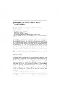
Figure 5, respectively. These results show that the proposed method outperforms G-LSSVR, local-LSSVR, and [15], and RMSE in Table 7 indicates the proposed method had the best generalization performance. In addition, the running time of the proposed methods in Table 8 is approximately 10 times shorter comparing with local-LSSVR method at least. In other words, the proposed method leads to a less computational time than local-LSSVR. As shown in Table 8, local-LSSVR needs more computational time. Additionally, the importance of selected different overlap factor 𝜆 is also compared by Table 9. Example 4. In this section, two hundred and ninety-six simulated data generated from a real Box-Jenkins [32] system are applied to the proposed method. These data points consisted of the gas flow rate signal 𝑥(𝑘) and the concentration of 𝐶𝑂2 which is described as the output of 𝑦(𝑘). Figure 6 shows the training data that include the input signal 𝑥(𝑘) and the output signal 𝑦(𝑘). To identify the model, we choose 𝑥𝑘 = [𝑥(𝑘), 𝑥(𝑘 − 1), 𝑦(𝑘 − 1), 𝑦(𝑘 − 2)] as
the input variables and 𝑦(𝑘) as the output variable. In this example, 5-folds cross-validation is employed to evaluate the performance. According to the cross-validation method, the (training/testing) RMSE and the computational time of the global LSSVR (G-LSSVR) approach, the local-LSSVR (LLSSVR) approach with 𝑀 = 41, 61, 81, and the proposed approach 𝑅 = 4, 8, 12 SRMs are summarized in Tables 10 and 11. From Tables 10 and 11, there is a little larger RMSE (training) for our technique than that of those approaches, the RMSE (testing) corresponding to our approach is smaller than that of them, and the run time for our technique is smaller than other local modeling approaches but litter bigger that global modeling techniques based on LSSVR. Figure 7 gives the comparisons between the actual output and the predicted output of our techniques. The importance of the selected different overlap factor 𝜆 is also compared in Table 12. As shown in Table 12, although the RMSE (training) corresponding to the overlap factor 𝜆 of 3.5 is less than that of 2.8, the RMSE (testing) corresponding to the overlap factor 𝜆 as 2.8 is less than that of as 3.4. That is to say, generalization
10
Mathematical Problems in Engineering
Table 7: Comparison results of the proposed method, [15], G-LSSVR and Local-LSSVR with the hyper-parameter set {1, 1000}, and the overlap factor 𝜆 as 1.5 are shown for Example 3. 𝑅: the number of the SRMs 3-SRMs 5-SRMS 7-SRMs 9-SRMs G-LSSVR Local-LSSVR M=21 training points M=41 training points M=61 training points M=81 training points
RMSE (Training) our approach 0.2523 0.2531 0.2287 0.2298 0.2922
RMSE (Testing) our approach 0.2546 0.2661 0.2537 0.2464 0.3185
[15] 0.2715 0.2659 0.2487 0.2465
1.8583 0.2332 0.2259 0.2433
[15] 0.2832 0.2762 0.2645 0.2583
1.8721 0.3383 0.3267 0.3561
Table 8: Comparison results of the proposed method, [15], G-LSSVR and Local-LSSVR with the hyper-parameter set {1, 1000}, and the overlap factor 𝜆 as 1.5 are shown for Example 3. R:the number of SRMs L-T(Second) Proposed approach T-T(Second) G-LSSVR M: Training points L-T(Second) Local-LSSVR T-T(Second)
3 0.2500 0.3281 T-T(Second): 0.1875 49 – 16.5469
5 0.2813 1.0938
7 0.2656 1.3438
9 0.3594 1.5313 L-T (Second): — 121 169 – – 17.9063 18.1719
81 – 16.7813
Table 9: Comparison results of the selected different overlap factor 𝜆 for our approach are shown for Example 3, where 𝑅 represents the number of SRMs, L-T the computational time for constructing all SRMs, and △𝑖 the number of data points for each training subset. 𝑅=5 𝜆=1.1 𝜆=2.5 𝑅=7 𝜆=1.1 𝜆=2.5
△1 106 268 △1 83 222
The total training data points △=501 △2 △3 △4 △5 106 118 118 117 183 266 183 267 △2 △3 △4 △5 99 98 97 98 147 147 215 222
△6 – – △6 98 221
△7 – – △7 83 215
RMSE (Training) 0.2531 0.2756
RMSE (Testing) 0.0142 0.2881
L-T (second) 0.2813 0.3438
0.2287 0.2818
0.2537 0.2894
0.2656 0.4063
Table 10: Comparison results of the proposed method, [15], G-LSSVR and Local-LSSVR with the hyper-parameter set {25, 1000}, and the overlap factor 𝜆 as 2.8 are shown for Example 4. 𝑅: the number of the SRMs 4-SRMs 8-SRMS 12-SRMs G-LSSVR Local-LSSVR M=41 training points M=61 training points M=81 training points
RMSE (Training) our approach 0.2544 0.2506 0.2491 0.2480 0.3328 0.3234 0.3237
[15] 0.1589 0.1365 0.1248
RMSE (Testing) our approach 0.3304 0.3321 0.3338 0.3355 0.3805 0.3666 0.3366
[15] 0.5163 0.4861 0.4218
Mathematical Problems in Engineering
11
Table 11: Computational time of the proposed method, G-LSSVR and Local-LSSVR with the hyperparameter set {25, 1000}, and the overlap factor 𝜆 as 2.8 are shown for Example 4, where the T-T represents total computational time for building the overall process of the proposed method and L-T represents the computational time for constructing all SRMs. R:the number of SRMs L-T(Second) T-T(Second) T-T(Second): 0.8281
Proposed approach G-LSSVR M: Training points
L-T(Second) T-T(Second)
Local-LSSVR
4 1.5938 2.4375
8 2.1407 3.6875
41 – 25.4375
61 – 25.7813
12 3.3437 4.8438 L-T (Second): — 81 – 26.3906
Table 12: Comparison results of the selected different overlap factor 𝜆 for our approach are shown for Example 4, where 𝑅 represents the number of SRMs, L-T the computational time for constructing all SRMs, and △𝑖 the number of data points for each training subset. The total training data points △=296, 𝜆=2.8 𝑅=4 𝐶𝑉1 𝐶𝑉2 𝐶𝑉3 𝐶𝑉4 𝐶𝑉5
△1 162 155 196 146 197
△2 △3 197 194 190 190 191 163 162 196 162 160 (𝐶𝑉1 + 𝐶𝑉2 + 𝐶𝑉3 + 𝐶𝑉4 + 𝐶𝑉5 )/5
△4 160 161 148 176 194
The total training data points △=296, 𝜆=3.5 △2 △3 193 219 213 197 222 200 183 218 219 208 (𝐶𝑉1 + 𝐶𝑉2 + 𝐶𝑉3 + 𝐶𝑉4 + 𝐶𝑉5 )/5
△4 217 200 192 205 193
performance in relatively smaller value of 𝜆 outperforms that of the large value. Additionally, in comparison of the [15], the proposed method only utilizes fewer hyperparameters to construct model, and the overlap factor 𝜆 is chosen in relatively smaller value to further reduce more computational time.
5. Conclusion In this paper, a fuzzy weighted least squares support vector regression (FW-LSSVR) method for nonlinear system modeling have been proposed and illustrated based on the advantages of fuzzy weighted mechanism and some ideas from LSSVR. Considering that each training subset is mutually independent, all SRMs can be constructed simultaneously and our method can largely reduce computational time. As shown in our experimental results, there have better superiorities in calculation time and modeling accuracy for our approach than those approaches such as local or global modeling method. It is noted that, run time for our technique is smaller than other local modeling approaches but litter bigger that global modeling techniques based on LSSVR.
Output signal y
△1 208 215 218 196 227
input signal x
𝑅=4 𝐶𝑉1 𝐶𝑉2 𝐶𝑉3 𝐶𝑉4 𝐶𝑉5
RMSE (Training)
RMSE (Testing)
L-T (second)
0.2236 0.2801 0.2883 0.2563 0.2236 0.2544 RMSE (Training)
0.4429 0.2374 0.2004 0.3282 0.4429 0.3304 RMSE (Testing)
0.2969 0.3438 0.3750 0.2656 0.3125 1.5938 L-T (second)
0.2151 0.2637 0.2761 0.2465 0.2151 0.2433
0.4381 0.2728 0.2066 0.3437 0.4381 0.3399
0.4219 0.3125 0.3906 0.3438 0.2969 1.7747
CO2 concentration
5 0 −5
0
50
100
150 Gas flow
200
250
300
0
50
100
150 X
200
250
300
70 60 50 40
Figure 6: The simulated data set obtained from Box and Jenkins is used to validate the proposed method.
Nevertheless, modeling accuracy for our approach has a considerable improvement than other techniques. Furthermore, in comparison with SVR, the proposed method only utilizes fewer hyperparameters to construct model, and the overlap
12
Mathematical Problems in Engineering R: 4 SRMs
CO2 concentration
65
[5] C. J. C. Burges, “A tutorial on support vector machines for pattern recognition,” Data Mining and Knowledge Discovery, vol. 2, no. 2, pp. 121–167, 1998.
60
[6] T. van Gestel, J. A. K. Suykens, B. Baesens et al., “Benchmarking least squares support vector machineclassifiers,” Machine Learning, vol. 54, no. 1, pp. 5–32, 2004.
55 50 45
0
50
100
150 X
200
250
300
Original data Proposed Method
[7] L. Zhang, W.-D. Zhou, P.-C. Chang, J.-W. Yang, and F.-Z. Li, “Iterated time series prediction with multiple support vector regression models,” Neurocomputing, vol. 99, pp. 411–422, 2013. [8] T. Quan, X. Liu, and Q. Liu, “Weighted least squares support vector machine local region method for nonlinear time series prediction,” Applied Soft Computing, vol. 10, no. 2, pp. 562–566, 2010.
Figure 7: Comparison of the proposed model outputs and original output data for Box and Jenkins example.
[9] T. Falck, P. Dreesen, K. de Brabanter, K. Pelckmans, B. de Moor, and J. A. K. Suykens, “Least-squares support vector machines for the identification of wiener-hammerstein systems,” Control Engineering Practice, vol. 20, no. 11, pp. 1165–1174, 2012.
factor 𝜆 is chosen in relatively smaller value than SVR to further reduce more computational time.
[10] L. Bako, G. Merc`ere, S. Lecoeuche, and M. Lovera, “Recursive subspace identification of Hammerstein models based on least squares support vector machines,” IET Control Theory & Applications, vol. 3, no. 9, pp. 1209–1216, 2009.
Data Availability The data used to support the findings of this study are available from the corresponding author upon request.
Conflicts of Interest The authors declared that they have no conflicts of interest to this work. We declare that we do not have any commercial or associative interest that represents a conflict of interest in connection with the work submitted.
Acknowledgments The research was partially funded by the training program of high level innovative talents of Guizhou ([2017]3, [2017]19), the Guizhou Province Natural Science Foundation in China (KY[2016]018, KY[2016]254), the Science and Technology Research Foundation of Hunan Province (13C333), the Science And Technology Project of Guizhou ([2017]1207, [2018]1179), and the Doctoral Fund of Zunyi Normal University (BS[2015]13, BS[2015]04).
References [1] D. Zhang, Z. Zhou, and X. Jia, “Networked fuzzy output feedback control for discrete-time Takagi-Sugeno fuzzy systems with sensor saturation and measurement noise,” Information Sciences, vol. 457/458, pp. 182–194, 2018. [2] M. De Gregorio and M. Giordano, “Background estimation by weightless neural networks,” Pattern Recognition Letters, vol. 96, pp. 55–65, 2017. [3] K. Li, J.-X. Peng, and E.-W. Bai, “A two-stage algorithm for identification of nonlinear dynamic systems,” Automatica, vol. 42, no. 7, pp. 1189–1197, 2006. [4] J. Suykens, L. Lukas, P. Van Dooren, B. De Moor, J. Vandewalle et al., “Least squares support vector machine classifiers: a large scale algorithm in,” in European Conference on Circuit Theory and Design, ECCTD, vol. 99, pp. 839–842, Citeseer, 1999.
[11] B.-Y. Sun, D.-S. Huang, and H.-T. Fang, “Lidar signal denoising using least-squares support vector machine,” IEEE Signal Processing Letters, vol. 12, no. 2, pp. 101–104, 2005. [12] B.-Y. Sun, D.-S. Huang, H.-T. Fang, and X.-M. Yang, “A novel robust regression approach of lidar signal based on modified least squares support vector machine,” International Journal of Pattern Recognition and Artificial Intelligence, vol. 19, no. 5, pp. 715–729, 2005. [13] H. B. Zheng, R. J. Liao, S. Grzybowski, and L. J. Yang, “Fault diagnosis of power transformers using multi-class least square support vector machines classifiers with particle swarm optimization,” IET Electric Power Applications, vol. 5, no. 9, pp. 691–696, 2011. [14] K. De Brabanter, J. De Brabanter, J. A. K. Suykens, and B. De Moor, “Approximate confidence and prediction intervals for least squares support vector regression,” IEEE Transactions on Neural Networks and Learning Systems, vol. 22, no. 1, pp. 110– 120, 2011. [15] C.-C. Chuang, “Fuzzy weighted support vector regression with a fuzzy partition,” IEEE Transactions on Systems, Man, and Cybernetics, Part B: Cybernetics, vol. 37, no. 3, pp. 630–640, 2007. [16] A. Ouyang, X. Peng, Y. Liu, L. Fan, and K. Li, “An Efficient Hybrid Algorithm Based on HS and SFLA,” International Journal of Pattern Recognition and Artificial Intelligence, vol. 30, no. 05, p. 1659012, 2016. [17] A. Miranian and M. Abdollahzade, “Developing a local leastsquares support vector machines-based neuro-fuzzy model for nonlinear and chaotic time series prediction,” IEEE Transactions on Neural Networks and Learning Systems, vol. 24, no. 2, pp. 207–218, 2013. [18] W. S. Cleveland and S. J. Devlin, “Locally weighted regression: an approach to regression analysis by local fitting,” Journal of the American Statistical Association, vol. 83, no. 403, pp. 596– 610, 1988. [19] V. Kecman and T. Yang, “Adaptive Local Hyperplane for regression tasks,” in Proceedings of the 2009 International Joint Conference on Neural Networks, IJCNN 2009, pp. 1566–1570, USA, June 2009.
Mathematical Problems in Engineering [20] A. Ouyang, X. Peng, J. Liu, and A. Sallam, “Hardware/Software Partitioning for Heterogenous MPSoC Considering Communication Overhead,” International Journal of Parallel Programming, vol. 45, no. 4, pp. 899–922, 2017. [21] E. E. Elattar, J. Goulermas, and Q. H. Wu, “Electric load forecasting based on locally weighted support vector regression,” IEEE Transactions on Systems, Man, and Cybernetics, Part C: Applications and Reviews, vol. 40, no. 4, pp. 438–447, 2010. [22] H. Yang, K. Huang, I. King, and M. R. Lyu, “Localized support vector regression for time series prediction,” Neurocomputing, vol. 72, no. 10–12, pp. 2659–2669, 2009. [23] H. Jiang and W. He, “Grey relational grade in local support vector regression for financial time series prediction,” Expert Systems with Applications, vol. 39, no. 3, pp. 2256–2262, 2012. [24] F. Wang, “A general learning framework using local and global regularization,” Pattern Recognition, vol. 43, no. 9, pp. 3120–3129, 2010. [25] J. A. K. Suykens and J. Vandewalle, “Least squares support vector machine classifiers,” Neural Processing Letters, vol. 9, no. 3, pp. 293–300, 1999. [26] D. E. Gustafson and W. C. Kessel, “Fuzzy clustering with a fuzzy covariance matrix,” in Proceedings of the IEEE Conference on Decision and Control including the 17th Symposium on Adaptive Processes, pp. 761–766, San Diego, Calif, USA, January 1979. [27] X. Liu, H. Fang, and Z. Chen, “A novel cost function based on decomposing least-square support vector machine for TakagiSugeno fuzzy system identification,” IET Control Theory & Applications, vol. 8, no. 5, pp. 338–347, 2014. [28] L. A. Zadeh, “Fuzzy sets,” Information and Computation, vol. 8, pp. 338–353, 1965. [29] J. M. Leski, “TSK-fuzzy modeling based on 𝜀-insensitive learning,” IEEE Transactions on Fuzzy Systems, vol. 13, no. 2, pp. 181– 193, 2005. [30] S. L. Chiu, “Fuzzy model identification based on cluster estimation,” Journal of Intelligent & Fuzzy Systems: Applications in Engineering and Technology, vol. 2, no. 3, pp. 267–278, 1994. [31] T. Takagi and M. Sugeno, “Fuzzy identification of systems and its applications to modeling and control,” IEEE Transactions on Systems, Man, and Cybernetics, vol. 15, no. 1, pp. 116–132, 1985. [32] G. E. P. Box and G. M. Jenkins, Time Series Analysis: Forecasting and Control, Holden-Day, San Francisco, Calif, USA, 1976.
13
Advances in
Operations Research Hindawi www.hindawi.com
Volume 2018
Advances in
Decision Sciences Hindawi www.hindawi.com
Volume 2018
Journal of
Applied Mathematics Hindawi www.hindawi.com
Volume 2018
The Scientific World Journal Hindawi Publishing Corporation http://www.hindawi.com www.hindawi.com
Volume 2018 2013
Journal of
Probability and Statistics Hindawi www.hindawi.com
Volume 2018
International Journal of Mathematics and Mathematical Sciences
Journal of
Optimization Hindawi www.hindawi.com
Hindawi www.hindawi.com
Volume 2018
Volume 2018
Submit your manuscripts at www.hindawi.com International Journal of
Engineering Mathematics Hindawi www.hindawi.com
International Journal of
Analysis
Journal of
Complex Analysis Hindawi www.hindawi.com
Volume 2018
International Journal of
Stochastic Analysis Hindawi www.hindawi.com
Hindawi www.hindawi.com
Volume 2018
Volume 2018
Advances in
Numerical Analysis Hindawi www.hindawi.com
Volume 2018
Journal of
Hindawi www.hindawi.com
Volume 2018
Journal of
Mathematics Hindawi www.hindawi.com
Mathematical Problems in Engineering
Function Spaces Volume 2018
Hindawi www.hindawi.com
Volume 2018
International Journal of
Differential Equations Hindawi www.hindawi.com
Volume 2018
Abstract and Applied Analysis Hindawi www.hindawi.com
Volume 2018
Discrete Dynamics in Nature and Society Hindawi www.hindawi.com
Volume 2018
Advances in
Mathematical Physics Volume 2018
Hindawi www.hindawi.com
Volume 2018