g-sddp generalized stochastic dual dynamic programming

G-SDDP GENERALIZED STOCHASTIC DUAL DYNAMIC PROGRAMMING

Ing. Jesus Velásquez Bermúdez, Eng. D. Chief Scientist, DO Analytics LLC - DecisionWare [email protected]

Fecha Documento: 11/12/2017

Versión Actualizada:

BENDERS THEORY

JACOBUS FRANCISCUS (JACQUES) BENDERS Jacobus Franciscus (Jacques) Benders (1 June 1924 - 9 January 2017) was a Dutch mathematician and Emeritus Professor of Operations Research at the Eindhoven University of Technology. He was the first Professor in the Netherlands in the field of Operations Research and is known for his contributions to Mathematical Programming. Benders studied mathematics at the Utrecht University, where he later also received his Ph. D. in 1960 with the thesis entitled "Partitioning in Mathematical Programming" under supervision of Hans Freudenthal. Late 1940s had started his career as statistician for the Rubber Foundation. In 1955 he moved to Shell laboratory in Amsterdam, where he researched mathematical programming problems concerning the logistics of oil refinery. He developed the technique known as Benders' decomposition, and used the results in his doctoral thesis. In 1963 Benders was appointed Professor of Operations Research at the Eindhoven University of Technology, being the first Professor in the Netherlands in that field. He retired at the Eindhoven University of Technology on May 31, 1989.

This conference analyzes the theory developed by J. F. Benders (BT) applied to the solution of dynamic problems using the Dynamic Programming and the Control Theory approaches. We call this methodology Generalized Dual Dynamic Programming (GDDP) which is based on the chained (nested) application of Bender´s Theory to a dynamic multi-period optimization problem. Many previous works must be kept in mind as an initial references, the works are related with Dynamic Nested Benders, and the methodology called Dual Dynamic Programming (DDP), a class of Nested Benders approach.

BENDERS THEORY Benders consideres a problem with two types of variables: x and y

Min cTx + f(y) subject to: F0 (y) = b0 A x + F (y) = b

An example of this: x associated with the operation and y with the investments

y

x

x  R+ yS

DUAL-ANGULAR STRUCTURE

BENDERS THEORY

MinY f(y) + Q(y) subject to : F0 (y) = b0 yS

Q(y) =

{

The Benders approach considers the function Q(y) that determines the optimum cost associate with x as a function of y Q(y) is determined by solving an optimization sub-problem, on the variable x, for multiple values of y

Minx cTx d

subject to: A x = b - F(y) x  R+

In this case, the sub-problem must be linear programming one

BENDERS THEORY


Q(y) =

{

Max  (b - F(y)) subject to:

A  c

Q(y)

can be defined based on the dual of the subproblem

BENDERS THEORY

2

MinY f(y) + Q(y) subject to : F0 (y) = b0 yS Q(y)  1 (b - F (y)) Q(y)  2 (b - F (y)) Q(y)  3 (b - F (y)) . . . Q(y)  NP (b - F (y))



3

A  C

1

4

5

The dual subproblem can be formulated in terms of the extreme points of its feasible zone

A  C

BENDERS THEORY

subject to :

The original problem can be formulated considering the variable y only, and all the cutting planes associated with the extreme points

F0 (y) = b0 yS

In practical terms, this problem has an infinite number of constraints

MinY f(y) + Q(y)

Q(y)  1 (b - F (y)) Q(y)  2 (b - F (y)) Q(y)  3 (b - F (y)) . . . Q(y)  NP (b - F (y))

To solve it, we should have a mechanism to generate extreme points of the dual feasible zone of the sub-problem that defines Q(y)

BENDERS THEORY

subject to :

The original problem can be formulated considering the variable y only, and all the cutting planes associated with the extreme points

F0 (y) = b0 yS

In practical terms, this problem has an infinite number of constraints

MinY f(y) + Q(y)

Q(y)  1 (b - F (y)) Q(y)  2 (b - F (y)) Q(y)  3 (b - F (y)) . . . Q(y)  NP (b - F (y))

To solve it, we should have a mechanism to generate extreme points of the dual feasible zone of the sub-problem that defines Q(y) Any feasible point  may be used to constraint Q(y), but, it may reduce the feasible zone and it is possible that the Benders procedure don’t converge to the optimal solution

BENDERS THEORY


The result is an algorithm based in cutting planes, that has the form:

Q(y)   k (b - F (y))

This is cutting plane is called

Q(y)   k (b - F (y)) k = 1, NP

BENDERS CUTTING PLANE FOR OPTIMALITY

BENDERS THEORY MODIFIED OPTIMALITY CUT

MinY f(y) + Q(y) +  × QA subject to : F0 (y) = b0 yS

The result is an algorithm based in cutting planes, that has the form:

Q(y) + QA   k (b - F (y))

This is cutting plane is called

Q(y) + QA   k (b - F (y)) k = 1, NP QA ≥ 0

MODIFIED BENDERS CUTTING PLANE FOR OPTIMALITY QA = Artificial Variable

This formulation ensures that the solution yk obtained in the iteration k is mathematically feasible for the cut included in the iteration k+1 (QA > 0), and it can be used as starting point of the search in the iteration k+1.

BENDERS THEORY

MinY f(y) + Q(y)

In case that feasible solution x does not exist, using the Farkas´s Theorem it should be to generate the following cutting plane:

subject to :

0   k (b - F (Y))

F0 (y) = b0 yS

where k corresponds to extreme ray of the feasible dual zone; This is cutting plane is called

Q(y)  k (b - F (y)) k = 1, NP 0   k (b - F (y)) k=1,RE

BENDERS CUTTING PLANE FOR FEASIBILITY If a feasible primal solution x does not exist then the dual solution is unbounded.

BENDERS THEORY

F0 (y) = b0 yS

y Feasible Zone

BENDERS THEORY

0  k (b - F (y))

Q(Y)  k (b - F (y))

Values of y that must be discarded because they can not be optimum

F0 (y) = b0 yS

y Feasible Zone

Values of y that must be discarded because they can not permitted feasible values of x

BENDERS THEORY

Miny f(y) + Q(y)

A structure of two levels is established to solve the problem

subject to: F0 (y) = b0 YS k Q(y)   (b - F (y)) k=1, ITERATIONS

Primal Variables



y

Min c x subject to: A x = b - F (y) x  R+

Dual Variables

The first level is the equivalent problem in terms of y, that is designated as the coordinator The second level is a subproblem for the variable x that generates extreme points for the coordinator problem The solution is obtained by exchanging information between the coordinator and the subproblem The coordinator proposes values of y and the subproblem generates dual variable 

ECONOMIC INTERPRETATION OF BENDERS THEORY Exist many interpretation of Benders Theory.

PRODUCTION MANAGER Miny f(y) + Q(y) subject to: F0 (y) = b0 YS k Q(y)   (b - F (y)) k=1, ITERATIONS

Primal Variables = Resources Assigments



y

Min c x subject to: A x = b - F (y) x  R+ INDUSTRIAL SYSTEM

Dual Variables = Marginal Productivity

For convenience, we assume that Benders coordinator represents an authority (a manager, a system operator, … ) that assign resources for many agents in a market or in a supply chain. Then, the first level define the vector y of resources assigned to the agents (sectors, factories, departments, … ). The second level is a subproblem related with the agents that generates information about the resources marginal productivity for each resource for each agent, or the prices that can pay the agents for the resources, represented by the dual variable 

ECONOMIC INTERPRETATION OF BENDERS THEORY Exist many interpretation of Benders Theory.

MARKET COORDINATOR Miny f(y) + Q(y) subject to: F0 (y) = b0 YS k Q(y)   (b - F (y)) k=1, ITERATIONS




y

Min c x subject to: A x = b - F (y) x  R+ RESOURCES MARKET


For convenience, we assume that Benders coordinator represents an authority (a manager, a system operator, … ) that assign resources for many agents in a market or in a supply chain. Then, the first level define the vector y of resources assigned to the agents (sectors, factories, departments, … ). The second level is a subproblem related with the agents that generates information about the resources marginal productivity for each resource for each agent, or the prices that can pay the agents for the resources, represented by the dual variable 

ECONOMIC INTERPRETATION OF BENDERS THEORY CORPORATIVE DECISION MAKERS Miny f(y) + Q(y) subject to: F0 (y) = b0 YS k Q(y)   (b - F (y)) k=1, ITERATIONS




y

Min c x subject to: A x = b - F (y) x  R+ SUPPLY CHAIN


Exist many interpretation of Benders Theory. For convenience, we assume that Benders coordinator represents an authority (a manager, a system operator, … ) that assign resources for many agents in a market or in a supply chain. Then, the first level define the vector y of resources assigned to the agents (sectors, factories, departments, … ). The second level is a subproblem related with the agents that generates information about the resources marginal productivity for each resource for each agent, or the prices that can pay the agents for the resources, represented by the dual variable 

CONVERGENCE OF BENDERS THEORY (MINIMIZATION)

c xk

Real Primal

cx

k Iterations

Estimated Dual Q(yk)

DYNAMIC PROGRAMMING

RICHARD ERNEST BELLMAN Richard Ernest Bellman was born in 1920 in New York City to nonpractising Jewish parents of Polish and Russian descent, Pearl (née Saffian) and John James Bellman, who ran a small grocery store on Bergen Street near Prospect Park, Brooklyn. He attended Abraham Lincoln High School, Brooklyn in 1937,[2] and studied mathematics at Brooklyn College where he earned a BA in 1941. He later earned an MA from the University of Wisconsin–Madison. During World War II he worked for a Theoretical Physics Division group in Los Alamos. In 1946 he received his Ph. D. at Princeton under the supervision of Solomon Lefschetz. Beginning 1949 Bellman worked for many years at RAND corporation and it was during this time that he developed the Dynamic Programming. Later in life, Richard Bellman's interests began to emphasize biology and medicine, which he identified as “the frontiers of contemporary science”. In 1967, he became founding editor of the Journal Mathematical Biosciences which specialized in the publication of applied mathematics research for medical and biological topics. In 1985, the Bellman Prize in Mathematical Biosciences was created in his honor, being award biannually to the journal's best research paper. Bellman was diagnosed with a brain tumor in 1973, which was removed but resulted in complications that left him severely disabled. He was a professor at the University of Southern California, a Fellow in the American Academy of Arts and Sciences (1975), a member of the National Academy of Engineering (1977), and a member of the National Academy of Sciences (1983). He was awarded the IEEE Medal of Honor in 1979, "for contributions to decision processes and control system theory, particularly the creation and application of dynamic programming“. His key work is the Bellman Equation.

LINEAR DYNAMIC PROGRAMMING

The Linear Dynamic Programming (DP) considers the solution of a dynamic problem of the form DP: = { min z = St=1,T ctTxt + dtTut | Atxt = bt - Et-1xt-1 - Btut "t=1,T Gtut = gt

"t=1,T

utR+,xtR+ "t=1,T }


Control Variables

xt-1 State Variables

ut

Atxt = bt - Et-1xt-1 - Btut Gtut = gt utR+ xtR+

Cost Function

ctTxt + dtTut

xt State Variables

DYNAMIC PROGRAMMING

Control Variables

ut Activity Levels: Production

xt-1

xt State Variables

State Variables Stocks Storages Cost Function

ctTxt + dtTut

DYNAMIC PROGRAMMING

Control Variables

ut Activity Levels: Production

xt-1

xt State Variables

State Variables Stocks Storages Cost Function

ctTxt + dtTut

DYNAMIC PROGRAMMING

Control Variables

xt-1

ut

THERM-GENERATION, FUEL CONSUMPTION, …

xt State Variables

State Variables WATER RELEASES, VOLUME RESERVOIRS, FUEL STORAGE, REMAINING CONTRACTS,...

Cost Function

ctTxt + dtTut +at (xt)

CLASSIC DYNAMIC PROGRAMMING

The Dynamic Programinng (DP) is based on the OPTIMALITY PRINCIPLE OF BELLMAN: “An optimum path has the property of the fact that anyone that it will be the initial decision and the state, the remaining decision shoulds constitute an optimum path with respect to the resulting state of the first decision“


The Linear Dynamic Programming (DP) considers the solution of a series of mathematical problems, one for each t, of the form DPt(xt-1): = { min zt = ctTxt + dtTut + at (xt) | Atxt = bt - Et-1xt-1 - Btut Gtut = gt utR+,xtR+ } where at (xt) is call the optimum future cost (“cost to go”) of the system for the period t+1 until T. The main idea of Bellman is that beginning in the last period, T, which does not include the future cost function aT(), it is possible to solve the problem associated with T-1 to obtain at-1 (xt-1). Then, in a backward recursive process, we can get the solution for first period, t=1, and solve the problem; finally, in a forward process, we can obtain the details of the solution.

DYNAMIC PROGRAMING

ut

xt-2

At-1xt-1 = bt-1 - Et-1xt-2

ut

xt-1

At xt = bt - Etxt-1

ut

xt

At+1 xt+1 = bt+1 – Et+1xt

ct-1Txt-1

ctTxt

ct+1Txt+1

+ dtTut

+ dtTut

+ dtTut

PHASE I - BACKWARD

xt+1

DYNAMIC PROGRAMING

PHASE II - FORWARD

ut

xt-2

At-1xt-1 = bt-1 - Et-1xt-2

ut

xt-1

At xt = bt - Etxt-1

ut

xt


ct-1Txt-1

ctTxt

ct+1Txt+1

+ dtTut

+ dtTut

+ dtTut

PHASE I - BACKWARD

xt+1

The original approach of DP is based in a numerical optimization process based on tables (state variables in t combined with state variables in t-1); for models with large quantity of state variables, this generates a big problem called "CURSE OF DIMENSIONALITY PROBLEM“ that implies that real problems with multiples state variables can not be solved exactly by DP due to dimension of tables that are required. Because, it is necessary to solve (st × st-1) reduced problems for each period t, where st represents the number of state variables in t. The complexity/dimensionality is related with the number of combinations that are necessary to solve the problem with enough precision.

DUAL DYNAMIC PROGRAMMING


In 1985, Pereira and Pinto presented a methodology that made it possible to apply the approach of Dynamic Programming (DP) to problems with multiple state variables without running into the "curse of dimensionality problem”. Pereira and Pinto extended Benders' partition theory (BT) to the multiplestage problem, which allowed the replacement of the discretization of the future cost function in the classic DP approach by a set of hyperplanes that defined it near to the optimal solution. The hyperplanes are generated using BT, that limits the subproblems to be linear. Dantzig & Infanger (1993) and Velásquez and others (1999) has similar formulation for the same problem. DDP is part of the “Nested Benders” methodologies, that are used to solve dynamic stochastic optimization problems based in random scenarios. There are many works over this type of use of Benders Theory.


DDP (DUAL DYNAMIC PROGRAMMING) & SDDP (STOCHASTIC DUAL DYNAMIC PROGRAMMING) are used intensively in the electric sector in the modeling of economic dispatch problem

CONCEPTUAL FORMULATION DP

DP

Control Variables

yt-1 State Variables

ut

Atyyt = b1t - Et-1yt-1 Btyt + Gtut = b2t

Stage Cost

ctTyt + dtTut

yt State Variables

CONCEPTUAL FORMULATION DDP

DP

DDP

Control Variables

xt-1

xt Atyxt = b1t - Et-1xt-1

State Variables

Stage Cost

ctTxt

State Variables


ut


Stage Cost

ctTyt + dtTut

yt State Variables

DDP: DUAL DYNAMIC PROGRAMING

xt-2

At-1xt-1 = bt-1 - Et-1xt-2

ct-1Txt-1

xt-1

At xt = bt - Etxt-1

xt

ctTxt

DYNAMIC PROGRAMMING STAGES


ct+1Txt+1

xt+1

DUAL DYNAMIC PROGRAMMING (DDP)

SUB-PROBLEM

COORDINATOR

xt-2

At-1xt-1 = bt-1 - Et-1xt-2

ct-1Txt-1

xt-1

At xt = bt - Etxt-1

xt

ctTxt



ct+1Txt+1

Xt+1

DUAL DINAMYC PROGRAMMING (DDP)

SUB-PROBLEM

COORDINATOR

xt-2

At-1xt-1 = bt-1 - Et-1xt-2

ct-1Txt-1

xt-1

At xt = bt - Etxt-1

xt

ctTxt



ct+1Txt+1

Xt+1

DUAL DINAMYC PROGRAMMING (DDP)

COORDINATOR SUB-PROBLEM

COORDINATOR

xt-2

At-1xt-1 = bt-1 - Et-1xt-2

ct-1Txt-1

xt-1

At xt = bt - Etxt-1

SUB-PROBLEM

xt

ctTxt

COORDINATOR


Xt+1

ct+1Txt+1

SUB-PROBLEM DYNAMIC PROGRAMMING STAGES

GDDP GENERALIZED DUAL DYNAMIC PROGRAMMING

GDDP: GENERALIZED DUAL DYNAMIC PROGRAMMING


GDDP Generalized Dual Dynamic Programming was developed based in theoretical considerations about the solution of dynamic optimization problems integrating the Benders Theory with the Dynamic Programming approach. G-SDDP Stochastic Generalized Dual Dynamic Programming is the stochastic extension of the GDDP.


DDP

xt-1


State Variables

Stage Cost

ctTxt

State Variables


DDP

GDDP

Control Variables

xt-1


State Variables

Stage Cost

ctTxt

State Variables


ut


Stage Cost

ctTyt + dtTut

yt State Variables


The conceptual approach of the GDDP maintains the difference between control variables and state variables. This distinction permits a more detailed algorithm in which the sub-problems are smaller than in the DDP. Then, the application of GDDP theory solves a coordinated sum of very simple problems. The GDDP formulation may be appropriate for industrial linear systems in which the state variables vector is associated with the amount of stock held and the level of resources in the facilities, and the control vector is associated with the production and distribution of products through the supply-chain. The GDDP family of optimization problems is used in the modeling of large supply-chains to support decision making at the tactical level (S&OP) in which the nonlinear characteristics can be, or must be, linearized.


GDDP (Velasquez 2002) is based on chained BT application to a multiperiodo optimization problem and corresponds to a generalization of DDP. GDDP: = { Min St=1,T ctTxt + dtTut | Ft xt = ft " t=1,T Atxt = bt - Et-1xt-1 - Btut " t=1,T Gtut = gt " t=1,T utR+ " t=1,T , xtR+ " t=1,T }

donde el vector xt representa las variables de estado y el vector ut las variables de control. At, Et, Bt, y Gt son matrices de relaciones funcionales, bt y gt son vectores de recursos, ct y dt vectores de costos y T el número de períodos del horizonte de planificación.


Control Variables

xt-1 State Variables

ut

Atxt = bt - Et-1xt-1 – Btut G tut = g t utR+ xtR+

Return

xt State Variables

ctTxt + dtTut + at(xt) State Cost

Control Future Cost Cost


GDDP: = { Min St=1,T ctTxt + dtTut | Ft xt = ft " t=1,T Atxt = bt - Et-1xt-1 - Btut " t=1,T Gtut = gt " t=1,T utR+ " t=1,T , xtR+ " t=1,T } x1 x2 x3

xT-2xT-1 xT

u1 u2 u3

uT-uuT-1 uT

.. . ..

The solution using Benders considers a two stage process. First ,we define the state variables xt as the coordination variables to proceed to decoupled the problem at temporary level. It implies to included in the coordinator decoupled Benders cuts. Thereinafter, the coordinator problem may be solved following one of the following alternatives : 1. IBC: It is solved as an integrated Benders coordinator problem.

.. .

.. . ..

DUAL-ANGULAR STRUCTURE

2. DDP: It is solved using the principles developed for DDP.

ECONOMIC INTERPRETATION OF BENDERS THEORY CORPORATIVE DECISION MAKERS Miny f(y) + Q(y) subject to: F0 (y) = b0 YS k Q(y)   (b - F (y)) k=1, ITERATIONS




y

Min c x subject to: A x = b - F (y) x  R+ INDUSTRIAL SYSTEM SUPPLY CHAIN RESOURCES MARKET


GDDP: GENERALIZED DUAL DYNAMIC PROGRAMMING INTEGRATED BENDERS COORDINATOR (IBC) CORPORATIVE DECISION MAKERS

CX: = { min z = St=1,T ctTxt + Wt(xt-1,xt) | Ft xt = ft " t=1,T Wt(xt-1,xt) + (tk)TEt-1xt-1+(tk)TAtxt qt(tk,dtk) "t=1,T "kIterations } tk

1k

Tk { xt-1 , xt }

{ x0 , x1 }

{ xT-1 , xT } t=T

t=1

min dtTut | Btut = bt - Et-1xt-1-Atxt Gtut = gt utR+ } INDUSTRIAL SYSTEM SUPPLY CHAIN RESOURCES MARKET

COUPLED BENDERS CUT

GDDP: GENERALIZED DUAL DYNAMIC PROGRAMMING INTEGRATED BENDERS COORDINATOR (IBC)


1k

Tk { xt-1 , xt }

{ x0 , x1 }

t=T

t=1

min dtTut | Btut = bt - Et-1xt-1-Atxt Gtut = gt utR+ }

{ xT-1 , xT }


DECOUPLED BENDERS CUTS



CX: = { min z = St=1,T ctTxt + Wt(xt-1,xt) | Ft xt = ft " t=1,T

Wt(xt-1,xt) = { min dtTut | Btut = bt - Et-1xt-1 - Atxt G tut = g t utR+ } "t=1,T xtR+ "t=1,T }

CX: corresponds to the coordinator problem where Wt(xt-1,xt) represents the optimum operation costs in the period t as a consequence of the border condition starting in the state xt-1 and finishing in the xt

Wt(xt-1,xt) corresponds to the objective function of the static operation subproblems for each period. In techno-economic terms, Wt(xt-1,xt) represents the supply function of the industrial system (or the supply chain) for the period t.


Wt(xt-1,xt) = { min dtTut | Btut = bt - Et-1xt-1 - Atxt G tut = g t utR+ } the dual problem that defines Wt(xt-1,xt) is

Wt(xt-1,xt) = { max tT[bt - Et-1xt-1 - Atxt] + dtTgt |

tTBt + dtTGt  dtT } where t represents the dual variables vector of Btut=bt-Et-1xt-1-Atxt and dt is the dual variables vector of Gtut = gt.

GDDP: GENERALIZED DUAL DYNAMIC PROGRAMMING DDP COORDINATOR

Considering the decoupled cuts generated by each static subproblem that defines Wt(xt-1,xt) the coordinator CX: is

CX: = { min z = St=1,T ctTxt + Wt(xt-1,xt) | Ft xt = ft " t=1,T Wt(xt-1,xt) + (tk)TEt-1xt-1+(tk)TAtxt qt(tk,dtk) "t=1,T "kIU } where IU represents the number of cuts generated for each subproblem and qt(,d) is a two argument t-index function that define a constant value

qt(,d) = Tbt + dTgt


The coordinator CX: is integrated by Benders cuts and the constraints Ft xt = ft , then it has a dynamic structure similar to the problem DDP: (only state variables) then CX: may solved it by using the DDP theory. The cuts that integrate the coordinator CX:

Wt(xt-1,xt) + (tk)TEt-1xt-1+(tk)TAtxt qt(tk,dtk) "t=1,T "kIU will be called Supply Function Benders Cuts (SF-BT)


The general coordinator can be solved based on the DDP principles. It can be demonstrated that the coordinator subproblem for each intermediate stage t (less than T) is

St=1,t

CGt: = { min z = [ ct Txt +Wt(xt-1,xt)] + at+1(xt) | Ft xt = ft "t=1,T

Wt(xt-1,xt) + (tk)TEt-1xt-1+(tk)TAtxt qt(tk,dtk) "t=1,t "kIU at+1(xt) + SkI1(t+1,j) yk,jt+1 (t+1k)TEtxt ftj "jIJ(t) xtR+ "t=1,T } The cuts that define at+1(xt) will be called Future Cost Benders Cuts (FC-BT)


The general coordinator can be solved based on the DDP principles. It can be demonstrated that the coordinator subproblem for each intermediate stage t (less than T) is

St=1,t

CGt: = { min z = [ ct Txt +Wt(xt-1,xt)] + at+1(xt) | Ft xt = ft "t=1,t

Wt(xt-1,xt) + (tk)TEt-1xt-1+(tk)TAtxt qt(tk,dtk) "t=1,t "kIU Wt(xt-1,xt) = SUPPLY FUNCTION at+1(xt) + SkI1(t+1,j) yk,jt+1 (t+1k)TEtxt ftj at+1(xt) = FUTURE "jCOST IJ(t) FUNCTION xtR+ "t=1,t }


x1

CGt: = { min z =

S t=1,t [ ct Txt +W t(xt-1,xt)] + at+1(xt) | Ft xt = ft "t=1,t W t(xt-1,xt) + (tk)TEt-1xt-1+(tk)TAtxt  qt(tk,dtk) "t(t) "kIU at+1(xt) + S kI1(t+1,j) y k,jt+1 (t+1k)TEtxt ftj "jIJ(t) xtR+ "t(t) }

1k

{ x0 , x1 }


yk,jt+1

CGt: = { min z =


tk

xT-1

CGt: = { min z =

S t=1,t [ ct Txt +W t(xt-1,xt)] + at+1(xt) | Ft xt = ft "t=1,t W t(xt-1,xt) + (tk)TEt-1xt-1+(tk)TAtxt  qt(tk,dtk) "t(t) "kIU

yk,jt+1

"jIJ(t) xtR+ "t(t) }

{ xT-1 , xT }

{ xt-1 , xt }

Tk

t=T

t=1




x1

CGt: = { min z =


1k

{ x0 , x1 }

yk,jt+1

CGt: = { min z =


tk

xT-1

CGt: = { min z =

S t=1,t [ ct Txt +W t(xt-1,xt)] + at+1(xt) | Ft xt = ft "t=1,t W t(xt-1,xt) + (tk)TEt-1xt-1+(tk)TAtxt  qt(tk,dtk) "t(t) "kIU

yk,jt+1

"jIJ(t) xtR+ "t(t) }

{ xT-1 , xT }

{ xt-1 , xt } t=T

t=1


Tk

GDDP: GENERALIZED DUAL DYNAMIC PROGRAMMING UNIFIED BENDERS CUTS

Bt , Gt, dt - TIME INDEPENDENT

Wt(xt-1,xt) = { max tT[bt-Et-1xt-1-Atxt] + dtTgt subject to

tTB + dtTG  dT }

Now we consider the special case when the dual feasibility zone of the problems that defines Wt(xt-1,xt) is static, which implies that the matrices Bt and Gt and the vector dt are time independent. Then, when we solve Wt(xt-1,xt) for a specific value of t we can generate SF-BT Benders cuts for all periods and the coordinator CX: In the case of Bt , Gt, dt are time dependent the cuts will be called UNIFIED BENDERS CUTS .











GDDP: GENERALIZED DUAL DYNAMIC PROGRAMMING INTEGRATED BENDERS COORDINATOR (IBC)


1k

Tk { xt-1 , xt }

{ x0 , x1 }

t=T

t=1


{ xT-1 , xT }




GENERALIZED DUAL DYNAMIC PROGRAMMING UNIFIED BENDERS CUTS – INTEGRATED COORDINATOR

CX: = { min z = St=1,T ctTxt + Wt(xt-1,xt) | Ft xt = ft " t=1,T Wt(xt-1,xt) + (tk)TEt-1xt-1+(tk)TAtxt qt(tk,dtk) "t=1,T "kIterations } k { xt-1 , xt }

UNIFIED BENDERS CUTS


Wt(xt-1,xt) = { max tT[bt-Et-1xt-1-Atxt] + dtTgt | tTB + dtTG  dT }

When Bt , Gt are TIME INDEPENDENT ? Bt and Gt are matrices that defines the topology and the technology of the industrial system. For short term and real-time operations this matrices don’t change because the industrial system is not changing (it is static); then in this case B and G are time independent. In the medium term and in the long term it is possible that this matrices change, but, in many cases is possible to orient the modeling using B and G time independent.


Wt(xt-1,xt) = { max tT[bt-Et-1xt-1-Atxt] + dtTgt | tTB + dtTG  dT }

When dt is TIME INDEPENDENT ? dt is the vector that defines the cost of the production operations. For real-time operations this vector may be time independent. We think that it is the majority of cases, but exists cases in which is not it isn’t true. Then it is necessary to analyze each case and to define which is the best way.

GENERALIZED DUAL DYNAMIC PROGRAMMING UNIFIED BENDERS CUTS – ECONOMIC INTERPRETATION

S

{ xt-1 , xt }

k min dtTut | Btut = bt - Et-1xt-1-Atxt Gtut = gt utR+ }

COBB-DOUGLAS PRODUCTION FUNCTION Q = f (K , T, … ) Production = f (Capital , Workforce. …)

Marginal Productivity

UNIFIED BENDERS CUTS Wt(xt-1,xt) + (tk)TEt-1xt-1+(tk)TAtxt qt(tk,dtk) "kIU

GENERALIZED DUAL DYNAMIC PROGRAMMING UNIFIED BENDERS CUTS – ECONOMIC INTERPRETATION

S

{ xt-1 , xt }

k min dtTut | Btut = bt - Et-1xt-1-Atxt Gtut = gt utR+ }

COBB-DOUGLAS PRODUCTION FUNCTION Q = f (K , T, … ) Production = f (Capital , Workforce. …)

Marginal Productivity

UNIFIED BENDERS CUTS Wt(xt-1,xt) + (tk)TEt-1xt-1+(tk)TAtxt qt(tk,dtk) "kIU

GENERALIZED DUAL DYNAMIC PROGRAMMING UNIFIED BENDERS CUTS - DDP COORDINATOR

x1

CGt: = { min z = St=1,t [ ct t +Wt(xt-1,xt)] + at+1(xt) | Wt(xt-1,xt) + (tk)TEt-1xt-1+(tk)TAtxt  qt(tk,dtk) "t(t) "kIU at+1(xt) + SkI1(t+1,j) yk,jt+1 (t+1k)TEtxt Tx

CGt: = { min z = St=1,t [ ct t +Wt(xt-1,xt)] + at+1(xt) | Wt(xt-1,xt) + (tk)TEt-1xt-1+(tk)TAtxt  qt(tk,dtk) "t(t) "kIU at+1(xt) + SkI1(t+1,j) yk,jt+1 (t+1k)TEtxt

xT-1

Tx

ftj "jIJ(t) xtR+ "t(t) }

CGt: = { min z =

St=1,t [ ct Txt +Wt(xt-1,xt)] + at+1(xt) | Wt(xt-1,xt) + (tk)TEt-1xt-1+(tk)TAtxt  qt(tk,dtk) "t(t) "kIU

ftj "jIJ(t) xtR+ "t(t) }

"jIJ(t) xtR+ "t(t) }

k x1

k

k xt

B , G, d - TIME INDEPENDENT

xT


x1



xT-1

Tx

ftj "jIJ(t) xtR+ "t(t) }

CGt: = { min z =


ftj "jIJ(t) xtR+ "t(t) }

"jIJ(t) xtR+ "t(t) }

k x1

k

k xt

xT

The previous problem can be solved in an asynchronous parallel form.

There is not a reason to synchronize the sub problems to a level of decomposition to accomplish the same iterations for each sub problem


x1



xT-1

Tx

ftj "jIJ(t) xtR+ "t(t) }

CGt: = { min z =


ftj "jIJ(t) xtR+ "t(t) }

"jIJ(t) xtR+ "t(t) }

k x1

k

k xt

xT

Then, we have a new problem: which the best way to choose the sub-problem to solve in the next iteration ? For real cases, the amount of sequences is “infinite”.


What can we do when

GDDP: = { Min St=1,T ctTxt + dtTut | Ft xt = ft " t=1,T Axt = bt - Et-1xt-1 - But " t=1,T Gut = gt " t=1,T utR+ " t=1,T xtR+ " t=1,T }

dt is TIME INDEPENDENT ? dt is the vector that defines the cost of the production operations.


What can we do when

GDDP: = { Min St=1,T ctTxt + dtTut | Ft xt = ft " t=1,T Axt = bt - Et-1xt-1 - But " t=1,T Gut = gt " t=1,T utR+ " t=1,T xtR+ " t=1,T }

dt is TIME INDEPENDENT ? dt is the vector that defines the cost of the production operations. It is possible to make some reformulation oriented to have an equivalent problem that have for all period a dual feasible zone independent of t.


What can we do when

GDDP: = { Min St=1,T ctTxt + dztTzt + dwTwt | Ft xt = ft " t=1,T Axt = bt - Et-1xt-1 - Bzzt - Bwwt " t=1,T Gzzt + Gwwt = gt " t=1,T {zt , wt }R+ " t=1,T , xtR+ " t=1,T }

where ut= {zt , wt } dt= {dzt , dw }

dt is TIME DEPENDENT ? dt is the vector that defines the cost of the production operations. May be possible to make a reformulation oriented to have an equivalent problem that have for all period a dual feasible zone independent of t. We can divide the vector of control variables in two type of variables: zt variables with cost dependent of t wt variables with cost independent of t. The variables zt will be part of the state variables and the control variables include wt .

DDP vs. GDDP

FULL PROBLEM

BENDERS MASTER

BENDERS SUBPROBLEM

DDP

GDDP

LP

LP

LP

YES

YES

MIP

MIP

LP

NO

YES

NLP

NLP

LP

NO

YES

MINLP

MINLP

LP

NO

YES

DDP vs. GDDP

FULL PROBLEM

BENDERS MASTER

BENDERS SUBPROBLEM

DDP

GDDP

LP

LP

LP

YES

YES

MIP

MIP

LP

NO

YES

NLP

NLP

LP

NO

YES

MINLP

MINLP

LP

NO

YES

GDDP is more robust than DDP

GDDP

IMPLEMENTATION & DETERMINISTIC EXPERIMENTS

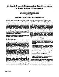
ECONOMIC DISPATCH OF ELECTRIC SYSTEMS

CONSUMER

RESERVOIR

~ HYDRO-ELECTRIC BUS

THERMO-ELECTRIC

12 8 6 1 24

Hydro Plants Reservoirs Thermal Plants Deficit Plant Hour Planning Horizon


CONSUMER

RESERVOIR

~ HYDRO-ELECTRIC HYDRO PLANTS - CONFIGURATION BUS

THERMO-ELECTRIC

12 8 6 1 24



CONSUMER

RESERVOIR

Actual Plants

~ HYDRO-ELECTRIC HYDRO PLANTS - CONFIGURATION BUS Actual Capacity Reservoirs (hm3) i01 17000 i02 2600 i05 200 i06 10000 i08 12500 THERMO-ELECTRIC i09 1000 i10 12400 i12 5000

Hydro Plant

Units

Capacity (MW)

Total Capacity (MW)

i01

Ui01 - Ui12

85

1020

i02

Ui01-Ui02 Ui03-Ui06 Ui07-Ui08

38 51 54

388

i03

Ui01 - Ui03

180

540

i04 i05 i06 i07 i08 i09

Ui01 Ui01-Ui02 Ui01-Ui04 Ui01-Ui02 Ui01-Ui04 Ui01-Ui03 Ui01-Ui03 Ui04-Ui06 Ui01-Ui02 Ui03-Ui05 Ui01-Ui02 Ui03-Ui04 Ui05-Ui06

40 130 200 15 300 125 380 380 20 52 150 180 280

40 260 800 30 1200 375

i10 i11

12 8 6 1 24


i12

Total Capacity (MW)

2280 196 1220

8349

ECONOMIC DISPATCH OF ELECTRIC SYSTEMS LINEAR MODELS Indexes i,i1 Hydro Plants - Index j Thermal Plants - Index t Time stages - Index Sets I={1,2,3,…,12} J={1,2,…, 6, D} T={t1, t2,…, t24} Up(I)

Hydro Plants set Thermal Plants set Time stages set Upstream hydro plant

Parameters Lt Energy Load ri Generation Characteristic Vmini Reservoir lower limit Vmaxi Reservoir upper limit Qmaxi Upper turbined outflow limit At,i Natural water inflow Gtminj Lower thermal generation limit Gtmaxj Upper thermal generation limit Ctj Generation cost

Variables GHt Hydraulic generation Vt,i Reservoir operating volume Qt,i Turbined outflow SPt,i Spillage outflow GTt,i Thermal Generation

ECONOMIC DISPATCH OF ELECTRIC SYSTEMS LINEAR MODELS Constraints Vmini ≤ Vt,i ≤ Vmaxi "t , " i Qmini ≤ 𝑸t,i ≤ 𝑸maxi " t , " i 0 ≤ 𝑺t,i " t , " i Gtmini ≤ 𝑮𝒕t,j ≤ 𝑮𝒕𝒎𝒂𝒙j " t , " jJ-{d} GHt - Si ri 𝑸t,i = 0 GHt + Sj 𝑮𝒕t,j = Lt

" t " t

Vt,i - Vt-1,i= At,i + Si1UP(i) (𝑸t,i1 + 𝑺t,i1) - (𝑸t,i + 𝑺t,i) "t , " i

Objective Function min z = St Sj 𝑪𝒕j 𝑮𝑻t,j

ECONOMIC DISPATCH OF ELECTRIC SYSTEMS LINEAR MODELS Control Variables

ut

xt-1

xt = { Vt,i , SPt,i , Qt,i , GHt }

ut = { GTt,j }

xt

State Variables

State Variables Reservoir Level Hydro Generation Spillage Water Releases

Thermal Generation

Cost Function

ctTxt + dtTut

GENERALIZED DUAL DYNAMIC PROGRAMMING (GDDP – LP Integrated Coordinator) LP

HYDRO-POWER SYSTEM tk

1k

Tk { xt-1 , xt }

{ x0 , x1 } t=1

LP THERMO-POWER SYSTEM

{ xT-1 , xT } t=T

LP


xt = { Vt,s , SPt,s , Qt,s , GHt } ut = { GTt,j }

THERMO-POWER SYSTEM

SEQUENCE OF THE SUBPROBLEMS

ORDER

TEM

CUB (Alternate)

Period

Energy Demand

Period

t01

26.52

t04

19.08

t02

25.50

t19

t03

23.85

t04

DEM

Energy Demand CUB -Order

Time Period

Energy Demand

DEM-Order

q01

t04

19.08

q01

41.58

q24

t03

23.85

q02

t03

23.85

q02

t06

24.96

q03

19.08

t20

38.43

q23

t02

25.50

q04

t05

26.25

t06

24.96

q03

t23

26.19

q05

t06

24.96

t18

37.62

q22

t05

26.25

q06

t07

27.63

t02

25.50

q04

t01

26.52

q07

t08

30.84

t21

36.24

q21

t24

26.88

q08

t09

30.27

t23

26.19

q05

t07

27.63

q09

t10

29.88

t13

34.11

q20

t16

28.98

q10

t11

29.28

t05

26.25

q06

t11

29.28

q11

t12

31.71

t15

32.79

q19

t22

29.55

q12

t13

34.11

t01

26.52

q07

t10

29.88

q13

t14

31.32

t12

31.71

q18

t09

30.27

q14

t15

32.79

t24

26.88

q08

t17

30.57

q15

t16

28.98

t14

31.32

q17

t08

30.84

q16

t17

30.57

t07

27.63

q09

t14

31.32

q17

t18

37.62

t08

30.84

q16

t12

31.71

q18

t19

41.58

t16

28.98

q10

t15

32.79

q19

t20

38.43

t17

30.57

q15

t13

34.11

q20

t21

36.24

t11

29.28

q11

t21

36.24

q21

t22

29.55

t09

30.27

q14

t18

37.62

q22

t23

26.19

t22

29.55

q12

t20

38.43

q23

t24

26.88

t10

29.88

q13

t19

41.58

q24

GDDP - GAMS CODE

DETERMINISTIC RESULTS LINEAR ECONOMIC DISPATCH Complexity: Real Variables: 1057 Constraints: 337 Elements no-Cero: 2245 Model

Order

Cota Dual

FULL

Cota Real 1866850.066

GAP (%)

T. Solution (secs)

Times FULL

0.0000

0.078

1.00

1.651

21.17

1.00

25.26

1.19

25.72

1.22

INTEGRATE MODEL

GDDP-UBC-O-CI

TEM

1866850.066

1866963.730

0.0061

GDDP-UBC-O-CI

DEM

1866850.066

1866963.730

0.0061

GDDP-UBC-O-CI

CUB

1866850.066

1866963.730

0.0001

GDDP-ST-CI

TEM

1866850.066 1866906.898CUTS 0.0030 2.775 DECOUPLED – INTEGRATED

DDP

TEM

1866850.066

GDDP-ST-DDP

TEM

1866850.066

1.970 UNIFIED CUTS 2.006

Times GDDP-UBC

35.58 1.68 COORDINATOR

162.77 DDP12.696 1866982.674 0.0071 42.912 550.15 DECOUPLED CUTS – DDP COORDINATOR 1866885.648

0.0019

7.69 25.99


Order

Cota Dual

FULL

Cota Real

GAP (%)

T. Solution (secs)

Times FULL

1866850.066

0.0000

0.078

1.00

Times GDDP-UBC

GDDP-UBC-O-CI

TEM

1866850.066

1866963.730

0.0061

1.651

21.17

1.00

GDDP-UBC-O-CI

DEM

1866850.066

1866963.730

0.0061

1.970

25.26

1.19

GDDP-UBC-O-CI

CUB

1866850.066

1866963.730

0.0001

2.006

25.72

1.22

GDDP-ST-CI

TEM

1866850.066

1866906.898

0.0030

2.775

35.58

1.68

DDP

TEM

1866850.066

1866885.648

0.0019

12.696

162.77

7.69

GDDP-ST-DDP

TEM

1866850.066

1866982.674

0.0071

42.912

550.15

25.99

FULL corresponds to the integrate model In this case, the complexity of the case does not justified the large scale methodologies; but it is useable to compare the large scale methodologies and to prove the convergence of all of them.


Order

Cota Dual

FULL

Cota Real

GAP (%)

T. Solution (secs)

Times FULL

1866850.066

0.0000

0.078

1.00

Times GDDP-UBC

GDDP-UBC-O-CI

TEM

1866850.066

1866963.730

0.0061

1.651

21.17

1.00

GDDP-UBC-O-CI

DEM

1866850.066

1866963.730

0.0061

1.970

25.26

1.19

GDDP-UBC-O-CI

CUB

1866850.066

1866963.730

0.0001

2.006

25.72

1.22

GDDP-ST-CI

TEM

1866850.066

1866906.898

0.0030

2.775

35.58

1.68

DDP

TEM

1866850.066

1866885.648

0.0019

12.696

162.77

7.69

GDDP-ST-DDP

TEM

1866850.066

1866982.674

0.0071

42.912

550.15

25.99

GDDP with UNIFIED CUTS is faster than any other large scale Benders methodology; independently of the order of selection the subproblem.


Order

Cota Dual

FULL

Cota Real

GAP (%)

T. Solution (secs)

Times FULL

1866850.066

0.0000

0.078

1.00

Times GDDP-UBC

GDDP-UBC-O-CI

TEM

1866850.066

1866963.730

0.0061

1.651

21.17

1.00

GDDP-UBC-O-CI

DEM

1866850.066

1866963.730

0.0061

1.970

25.26

1.19

GDDP-UBC-O-CI

CUB

1866850.066

1866963.730

0.0001

2.006

25.72

1.22

GDDP-ST-CI

TEM

1866850.066

1866906.898

0.0030

2.775

35.58

1.68

DDP

TEM

1866850.066

1866885.648

0.0019

12.696

162.77

7.69

GDDP-ST-DDP

TEM

1866850.066

1866982.674

0.0071

42.912

550.15

25.99

GDDP with UNIFIED CUTS is faster than GDDP with DECOUPLED CUTS


Order

Cota Dual

FULL

Cota Real

GAP (%)

T. Solution (secs)

Times FULL

1866850.066

0.0000

0.078

1.00

Times GDDP-UBC

GDDP-UBC-O-CI

TEM

1866850.066

1866963.730

0.0061

1.651

21.17

1.00

GDDP-UBC-O-CI

DEM

1866850.066

1866963.730

0.0061

1.970

25.26

1.19

GDDP-UBC-O-CI

CUB

1866850.066

1866963.730

0.0001

2.006

25.72

1.22

GDDP-ST-CI

TEM

1866850.066

1866906.898

0.0030

2.775

35.58

1.68

DDP

TEM

1866850.066

1866885.648

0.0019

12.696

162.77

7.69

GDDP-ST-DDP

TEM

1866850.066

1866982.674

0.0071

42.912

550.15

25.99

GDDP with UNIFIED CUTS is 8 times faster than DDP GDDP with DECOUPLED CUTS is 4.5 times faster than DDP


Order

Cota Dual

FULL

Cota Real

GAP (%)

T. Solution (secs)

Times FULL

1866850.066

0.0000

0.078

1.00

Times GDDP-UBC

GDDP-UBC-O-CI

TEM

1866850.066

1866963.730

0.0061

1.651

21.17

1.00

GDDP-UBC-O-CI

DEM

1866850.066

1866963.730

0.0061

1.970

25.26

1.19

GDDP-UBC-O-CI

CUB

1866850.066

1866963.730

0.0001

2.006

25.72

1.22

GDDP-ST-CI

TEM

1866850.066

1866906.898

0.0030

2.775

35.58

1.68

DDP

TEM

1866850.066

1866885.648

0.0019

12.696

162.77

7.69

GDDP-ST-DDP

TEM

1866850.066

1866982.674

0.0071

42.912

550.15

25.99

GDDP with INTEGRATE COORDINATOR is 15.5 times faster than GDDP with DDP COORDINATOR


Order

Cota Dual

FULL

Cota Real

GAP (%)

T. Solution (secs)

Times FULL

1866850.066

0.0000

0.078

1.00

Times GDDP-UBC

GDDP-UBC-O-CI

TEM

1866850.066

1866963.730

0.0061

1.651

21.17

1.00

GDDP-UBC-O-CI

DEM

1866850.066

1866963.730

0.0061

1.970

25.26

1.19

GDDP-UBC-O-CI

CUB

1866850.066

1866963.730

0.0001

2.006

25.72

1.22

GDDP-ST-CI

TEM

1866850.066

1866906.898

0.0030

2.775

35.58

1.68

DDP

TEM

1866850.066

1866885.648

0.0019

12.696

162.77

7.69

GDDP-ST-DDP

TEM

1866850.066

1866982.674

0.0071

42.912

550.15

25.99

GDDP is faster than DDP

UNIT COMMITMENT OF ELECTRIC SYSTEMS MIXED LINEAR MODEL

CONSUMER

RESERVOIR


THERMO-ELECTRIC

12 8 6 1 24

Hydro Plants Reservoirs Thermal Plants (Start – Stop) Deficit Plant Hour Planning Horizon

MUST RUN POWER PLANTS (COAL - NUCLEAR) START/STOP THERMO-ELECTRIC CONTINUOUS OPERATION

STt,j × GMINt,j ≤ GTt,p ≤ STt,j × GMAXt,j STt,j - STt-1,j ≤ SRt,j SRt,j  {0,1}  START THERMO-ELECTRIC STt,J  {0,1}  THERMO-ELECTRIC STATE (off, on)

COST: CVGTt,p × GTt,J + CARRJ × SRt,V

MUST RUN POWER PLANTS (COAL - NUCLEAR) START/STOP THERMO-ELECTRIC CONTINUOUS OPERATION

STt,p - STt-1,p ≤ SRt,p

STt,j

-

STt-1,j

≤

SRt,j

1 0 1 0

-

0 0 1 1

≤ ≤ ≤ ≤

1 0 0 0

COST: CVGTt,p × GTt,p + CARRp × SRt,p

UNIT COMMITMENT OF ELECTRIC SYSTEMS MIXED LINEAR MODEL Control Variables

ut

xt-1

ut = { GTt,j }

xt

State Variables

State Variables Reservoir Level Hydro Generation Spillage Water Releases Start Thermal Plants State Thermal Plants

Thermal Generation

Cost Function

xt = { Vt,i , St,i , Qt,i , GHt , SRt,j STt,j}

ctTxt + dtTut

GENERALIZED DUAL DYNAMIC PROGRAMMING (GDDP – MIP Integrated Coordinator) MIP

HYDRO-POWER SYSTEM START/STOP THERMAL PLANTS tk

1k

Tk { xt-1 , xt }

{ x0 , x1 } t=1


{ xT-1 , xT } t=T

LP


xt = { Vt,i , St,i , Qt,i , GHt , SRt,j STt,j} ut = { GTt,j }

THERMO-POWER SYSTEM

BENDERS – INEXACT CUTS FOR MIP COORDINATORS

INEXACT CUTS

Q(y) + ek   k (b - F (y))

e1  e2  e3 

… ek

... e  0


c xk

Real Primal

cx

k Iterations


CONVERGENCE OF BENDERS THEORY INEXACT SOLUTIONS - INEXACT CUTS

c xk

Real Primal

cx

k Iterations


e1


c xk

Real Primal

cx ek


e1

k Iterations


c xk

Real Primal

cx

e =0 ek


e1

k Iterations

BENDERS – VARIATIONS FOR MIP COORDINATORS

INEXACT SOLUTIONS

[ { f(yk) + Q(yk) } - { f(y*) + Q(y*) } ] [ f(y*) + Q(y*) ]

≤ qk

yk  Feasible Zone of Benders Coordinator y* Optimal Solution

q1  q2  q3 

… qk

... q  0


c xk

Real Primal

cx

k Iterations


CONVERGENCE OF BENDERS THEORY INEXACT SOLUTIONS

c xk

Real Primal

cx

k Iterations


q1

CONVERGENCE OF BENDERS THEORY INEXACT SOLUTIONS

c xk

q1

Real Primal qk

cx

k Iterations



c xk

q1

Real Primal qk

cx q =0


k Iterations

DETERMINISTIC RESULTS MIP UNIT COMMITMENT

GAP

Solution Time (secs)

0.00000

0.373

0.00000

1.277

GDDP-UBC-O-CI

0.0000

1.947

FULL

0.00000

0.896

0.00000

4.673

GDDP-UBC-O-CI

0.00000

5.424

FULL

0.00000

1.309

0.00002

17.546

GDDP-UBC-O-CI

0.00000

13.126

FULL

0.00000

27.466

0.00002

44.582

GDDP-UBC-O-CI

0.00000

16.540

FULL

0.00060

1001.147

0.00007

75.094

GDDP-UBC-O-CI

0.00000

33.032

FULL

0.00020

1003.005

0.00008

185.228

0.00000

130.555

Model

Periods

FULL GDDP-ST-CI

GDDP-ST-CI

GDDP-ST-CI

GDDP-ST-CI

GDDP-ST-CI

GDDP-ST-CI GDDP-UBC-O-CI

24

48

96

192

384

768

Real Variables

Binary Variables

576

288

769

3391

2214

384

1537

6799

4225

1152

3073

13615

9217

1536

6145

27427

18433

3072

12289

54511

36865

6144

24577

109039

Constraints Non-ceroes

In all cases was stablished that maximum process time was 1000 seconds, in two cases the FULL problem don’t get a solution under the maximum time.

GDDP: CONCLUSIONS

1. In all cases, the GDDP algorithm converge to optimal solution 2. GDDP speed up the solution of mathematical optimization problems with LP & MIP Benders Coordinators. 3. GDDP approach is faster than DDP 4. GDDP-UBC (one unified problem generator of cuts for all periods) is faster than GDDP-ST (one standard generator for each period).

5. For the master problem, the integrated coordinator (IBC) is faster than the DDP coordinator. 6. GDDP-UBC detected the upper bound very rapidly, but take time to prove its optimality. 7. GDDP-UBC plus inexact solutions may be faster than optimal solutions for MIP Benders Coordinators. 8. The relation between solution time and dimensionality of the deterministic problem (amount of periods) is lineal, that implies that is possible to manage very large problems, in time.

G-SDDP GENERALIZED STOCHASTIC DUAL DYNAMIC PROGRAMMING

G-SDDP: GENERALIZED STOCHASTIC DUAL DYNAMIC PROGRAMMING

G-SDDP corresponds to a particular formulation of the linear multi-stage stochastic optimization problem lineal (MS-SLP) with the following structure. G-SDDP: = { Min Sh qh St ct,h

Ft,h xt,h = ft,h

Tx

t,h

+ dt,h

Tu

t,h

] |

" t=1,T "hN

At,h xt,h + Bt,h ut,h = bt,h - Et,hxt-1,h "t "hN

"t "nN

Gt,h ut,h = gt,h

ut,hR+ "t "hN xt,h

R+

"t "hN }

Where: xt,h ut,h

state and vector control variables

At,h , Et,h , Bt,h , and Gt,h functional matrices bt,h , gt,h resources vectors ct,h , dt,h cost vectors all of them may be dependent on the stochastic process;

qh T

probability of the scenario h amount of periods (stages)


G-SDDP corresponds to a particular formulation of the linear multi-stage stochastic optimization problem lineal (MS-SLP) with the following structure. G-SDDP: = { Min Sh qh St ct,h

Ft,h xt,h = ft,h

Tx

t,h

+ dt,h

Tu

t,h

] |

" t=1,T "hN

At,h xt,h + Bt,h ut,h = bt,h - Et,hxt-1,h "t "hN

"t "nN

Gt,h ut,h = gt,h

ut,hR+ "t "hN xt,h

R+

"t "hN

Where: xt,h ut,h

At,h , Et,h , Bt,h , and Gt,h functional matrices bt,h , gt,h resources vectors ct,h , dt,h cost vectors all of them may be dependent on the stochastic process;

qh T N(t)

NON-ANTICIPATIVE CONSTRAINTS uAt,n = ut,h

"t

" nN(t) "h(n)

xAt,n = xt,h

"t

" nN (t) "h(n) }

state and vector control variables

B(n)

probability of the scenario h amount of periods (stages) nodes of decision tree related with period t scenarios related with node n


Following the principles of GDDP, an alternative for solving G-SDDP: is based on partition and decomposition using BT to structure the coordinated solution of multiple smaller subproblems. Interpreted from the point of view of production systems, G-SDDP resolves at every stage and for each node in the decision tree, a static sub-problem oriented to produce information concerning the supply function and: i) using recursion "backward" to combine this information with the functions of future costs, or ii) solving the integrated coordinator, in order to establish the optimal strategy, The supply function and future cost functions are built from the hyperplanes that define them, which are generated using BT.

G-SDDP: GENERALIZED STOCHASTIC DUAL DYNAMIC PROGRAMMING INTEGRATED BENDERS COORDINATOR (IBC)


1k

Tk { xt-1 , xt }

{ x0 , x1 } t=1


{ xT-1 , xT } t=T




G-SDDP: G-SDDP - INTEGRATED COORDINATOR (IBC) GENERALIZED STOCHASTIC DUAL DYNAMIC PROGRAMMING INTEGRATED BENDERS COORDINATOR (IBC)

CX: = { min z = St=1,T ct,hTxt,h + Wt,h(xt-1,h,xt,h ) | Ft,h xt,h = ft,h " t=1,T Wt,h(xt-1,h,xt,h)+(t,hk)TEt-1,h xt-1,h+(tk)TAt,hxt,hqt,h(t,hk,dt,hk) "t=1,T "kITE(t,h) }

tk

1k

Tk { xt-1 , xt }

{ x0 , x1 }

{ xT-1 , xT }

t=1 t=T

min dtTut | Bt ut,h = bt,h - Et-1 xt-1,h - At,hxt,h Gt.h ut,h = gt ut,hR+ }



G-SDDP - INTEGRATED COORDINATOR (IBC)

NON-ANTICIPATIVE CONSTRAINTS "t " nN(t) "h(n) "t " nN (t) "h(n)

uAt,n = ut,h xAt,n = xt,h


tk

1k

Tk { xt-1 , xt }

{ x0 , x1 }

{ xT-1 , xT }


tk

1k

{ xt-1 , xt }

{ x0 , x1 }

t=1

Tk

t=1 t=T


{ xT-1 , xT }


t=T









tk

1k

Tk { xt-1 , xt }

{ x0 , x1 }

{ xT-1 , xT }


tk

1k

{ xt-1 , xt }

{ x0 , x1 }

t=1

Tk

t=1 t=T


{ xT-1 , xT }


t=T






tk

1k

Tk { xt-1 , xt }

{ x0 , x1 }

{ xT-1 , xT }

tk

1k

{ xt-1 , xt }

{ x0 , x1 }

t=1

Tk

t=1 t=T


{ xT-1 , xT }


t=T





G-SDDP - INTEGRATED BENDERS COORDINATOR (IBC) UNIFIED BENDERS CUTS B , G, d - TIME INDEPENDENT

Tk

{ xt-1 , xt }

UNIFIED BENDERS CUTS

G-SDDP

IMPLEMENTATION & STOCHASTIC EXPERIMENTS

G-SDDP - INTEGRATED BENDERS COORDINATOR (IBC) DYNAMIC & STOCHASTIC

HYDRO-POWER SYSTEM SCENARIO COORDINATOR – INTERTEMPORAL COORDINATOR

tk

1k

Tk { xt-1 , xt }

{ x0 , x1 }

{ xT-1 , xT }

t=1

tk

1k

Tk { xt-1 , xt }

{ x0 , x1 }

{ xT-1 , xT }

t=1 t=T

t=T


G-SDDP – SCENARIO COORDINATION



HYDRO-POWER SYSTEM

HYDRO-POWER SYSTEM

SCENARIO 1

SCENARIO H

G-SDDP - LAGRANGEAN COORDINATOR (LC)

T

SCENARIO LAGRANGEAN COORDINATOR

k

{ xt-1 , xt }

HYDRO-POWER SYSTEM

HYDRO-POWER SYSTEM

GDDP DYNAMIC COORDINATOR

GDDP DYNAMIC COORDINATOR

SCENARIO 1

SCENARIO H

tk

1k { x0 , x1 }

Tk { xt-1 , xt }

{ xT-1 , xT }

t=T

tk

1k { x0 , x1 }

Tk { xt-1 , xt }

{ xT-1 , xT }

t=T


G-SDDP - INTEGRATED BENDERS COORDINATOR (IBC) UNIFIED BENDERS CUTS

CX: = { min z = Sh qh St=1,T ct,hTxt,h + Wt(xt-1,h,xt,h ) | Ft,h xt,h = ft " t=1,T "h=1,H k T Wt(xt-1,h,xt,h) + (t,h ) Et-1,h xt-1,h+(tk)Tatxt,h qt(t,hk,dt,hk) "t=1,T "h=1,H "kIterations uAt,n = ut,h "t " nN(t) "h(n) xAt,n = xt,h "t " nN (t) "h(n) } Tk

{ xt-1 , xt }

B , G, d - TIME INDEPENDENT

STOCHASTIC ECONOMIC DISPATCH LINEAR MODEL

Scena rios

Model

T. Solution (secs)

Times FULL

Times G-SDDP-UBC-O

Algorithm CO

Algorithm SP

GAMS

0.402

1.00

0.00000

4.297

10.69

1.00

Default

Dual Simplex

SLINK

0.00011

458.00

1139.30

106.59

Default

NA

SLINK+GUSS

0.00000

25.172

62.61

5.85

Default

Dual Simplex SLINK+GUSS

0.606

1.00

0.00000

7.005

11.56

1.00

Default

Dual Simplex

SLINK

0.00017

687.00

1133.66

98.07

Default

NA

SLINK+GUSS

0.00000

53.092

87.607

7.58

Default

GAP

FULL G-SDDP-UBC-O-CI SDDP

10

G-SDDP-UBC-O-DDP FULL

G-SDDP-UBC-O-CI SDDP G-SDDP-UBC-O-DDP

20


FULL corresponds to the integrate model (equivalent deterministic)

The complexity of the case does not justified the large scale methodologies; but it is useable to compare the large scale methodologies and to prove the convergence of all of them.

STOCHASTIC ECONOMIC DISPATCH LINEAR MODEL

Model

Scena rios

T. Solution (secs)

Times FULL

Times G-SDDP-UBC-O

Algorithm CO

Algorithm SP

GAMS

0.402

1.00

0.00000

4.297

10.69

1.00

Default

Dual Simplex

SLINK

0.00011

458.00

1139.30

106.59

Default

NA

SLINK+GUSS

0.00000

25.172

62.61

5.85

Default


0.606

1.00

0.00000

7.005

11.56

1.00

Default

Dual Simplex

SLINK

0.00017

687.00

1133.66

98.07

Default

NA

SLINK+GUSS

0.00000

53.092

87.607

7.58

Default

GAP

FULL G-SDDP-UBC-O-CI SDDP

10

G-SDDP-UBC-O-DDP FULL

G-SDDP-UBC-O-CI SDDP G-SDDP-UBC-O-DDP

20

The experiments show that G-SDDP is 100 times faster than SDDP


BENDERS – INEXACT SOLUTIONS FOR MIP COORDINATORS

Model Scenarios FULL G-SDDP-UBC-O-CI 20 G-SDDP-UBC-O-CI FULL 50 G-SDDP-UBC-O-CI FULL 100 G-SDDP-UBC-O-CI

eps CI % 0 0 0.5

GAP

0.5

0 0.002

0.5

0 0

T. Solution (secs) 38.509 124.395 12.101 1221.176 126.837 MEM 386.657

MEM = Out of memory

Times 3.18 10.28 1.00 9.63 1.00

STOCHASTIC UNIT COMMITMENT MIXED MODEL – UNIFIED CUTS + INEXACT SOLUTIONS Time

Time/Scenario

(secs)

(secs/scenario)

20

12.01

0.601

50

127

2.537

100

387

3.867

200

1092

5.461

500

1321

2.642

1000

1570

1.570

2000

2524

1.262

4000

4634

1.159

8000

10852

1.356

Scenarios

Scenarios

Variables

V. Binaries

Constraints

NO-Ceros

20

29,924

5,760

16,221

69,521

50

67,224

14,400

40,551

173,801

100

134,444

28,800

81,101

347,601

200

268,844

57,600

162,201

695,201

500

672,044

144,000

440,501

1,738,001

1000

1,344,044

288,000

811,001

3,476,001

2000

2,688,044

576,000

1,622,001

6,952,001

4000

5,376,044

1,152,000

3,244,001

13,904,001

8000

10,752,044

2,304,000

6,488,001

27,808,001

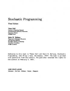
STOCHASTIC UNIT COMMITMENT MIXED MODEL – UNIFIED CUTS + INEXACT SOLUTIONS 12000 TIME (sec)

Time

Time/Scenario

20 50 100 200 500 1000 2000 4000

(secs) 12.01 127 387 1092 1321 1570 2524 4634

(secs/scenario) 0.601 2.537 3.867 5.461 2.642 1.570 1.262 1.159

8000

10852

1.356

Scenarios 10000

8000

6000

4000

2000

SCENARIOS

0 0

1000

2000

3000

4000

5000

6000

7000

8000

STOCHASTIC UNIT COMMITMENT MIXED MODEL – UNIFIED CUTS + INEXACT SOLUTIONS

6 Scenarios

5

4

3

Solution Time

Time/Scenario

(secs)

(secs/scenario)

20

12.01

0.601

50

127

2.537

100

387

3.867

200

1092

5.461

500

1321

2.642

1000

1570

1.570

2000

2524

1.262

4000

4634

1.159

8000

10852

1.356

2

1

0 0

1000

2000

3000

4000

5000

6000

7000

8000

G-SDDP STATISTICAL CONVERGENCE STOCHASTIC UNIT COMMITMENT MIXED NON-LINEAR MODEL

G-SDDP accepts the statistical converge criterium, based in the precision of the estimator of the objective function value, or another random variable of the model.

Strategy

Scenarios

Step

Scenarios +

Mean

Deviation

SSE Goal

SSE

Formula Formula Formula Incremental Incremental

20 30 100 20 20

195 196 0 50 100

215 226 100 120 120

39716 39768 41630 41200 41200

20698 20776 19151 20534 20534

1985.79 1988.38 2081.50 2060.01 2060.01

1411.62 1381.97 1915.06 1874.53 1874.53

SEE = Standard Error Estimator

T. Solution (secs) 77.827 93.286 95.419 68.741 44.646

ECONOMIC DISPATCH OF ELECTRIC SYSTEMS MIXED NON-LINEAR MODELS

CONSUMER

RESERVOIR


THERMO-ELECTRIC

1 12 8 6 1 24

Water Pumping Station Hydro Plants Reservoirs Thermal Plants Deficit Plant Hour Planning Horizon

ECONOMIC DISPATCH OF ELECTRIC SYSTEMS MIXED NON-LINEAR MODELS Indexes i,i1 Hydro Plants - Index j Thermal Plants - Index t Time stages - Index Sets I={1,2,3,…,12} J={1,2,…, 6, D} T={t1, t2,…, t24} Up(i) BR(i) BR(i)

Hydro Plants set Thermal Plants set Time stages set Upstream hydro plant Pumping station i to i1 Pumping station i1 from i1

Parameters Lt Energy Load ri Generation Characteristic Vmini Reservoir lower limit Vmaxi Reservoir upper limit Qmaxi Upper turbined outflow limit At,i Natural water inflow Gtminj Lower thermal generation limit Gtmaxj Upper thermal generation limit Ctj Generation cost PUmini Pumping station lower limit PUmaxi Pumping station upper limit

Variables GHt Hydraulic generation Vt,i Reservoir operating volume Qt,i Turbined outflow SPt,i Spillage outflow GTt,i Thermal Generation PUt,i,i1 PWt,i

Water pumped from i to i1 Power used in pumping station i

BPt,i

Binary variable to control pumping

Cost Parameters Ctj Generation cost Cu1i Pumping cost (linear coefficient) Cu2i Pumping cost (quadratic coefficient)

ECONOMIC DISPATCH OF ELECTRIC SYSTEMS MIXED NON-LINEAR MODEL Constraints Vmini ≤ Vt,i ≤ Vmaxi "t , " i (1 - BPt,i) × Qmini ≤ 𝑸t,i ≤ 𝑸maxi × (1 - BPt,i) " t , " i 0 ≤ 𝑺t,i Gtmini ≤ 𝑮𝒕t,j ≤ 𝑮𝒕𝒎𝒂𝒙j

" t , " i " t , " jJ-{d}

GHt - Si ri 𝑸t,i = 0 GHt + Sj 𝑮𝒕t,j = Lt

" t " t

Vt,i - Vt-1,i = At,i + Si1UP(i) [ (𝑸t,i1 + 𝑺t,i1) - (𝑸t,i + 𝑺t,i ) ] + Si1BR(i) PUt,i1,i - Si1RB(i) PUt,i,i1 PWt,i = 9.8 × 0.001 × Si1BR(i) PUt,i

"t , " iIPU

(1 - BPt,i) × PUmainxi ≤ Si1BR(i) PWt,i,i1 ≤ (1 - BPt,i) × PUmaxi

"t , " iIPU

Objective Function min z = St [ Sj 𝑪𝒕j 𝑮𝑻t,j + Si ( 𝑪u1i 𝑷𝑾t,i + 𝑪u2i 𝑷𝑾𝟐t,i ) ]

ECONOMIC DISPATCH OF ELECTRIC SYSTEMS MIXED NON-LINEAR MODEL

Periods

Model Type

Scenarios

1 NLP

20

24 50 MI NLP

1

5

Dual Bound 2718504

Primal Bound 2718504

2718499

2718499

0

4.102

XPRESS

2718507

2718507

0

4.905

MINOS

2718504

2718504

0

63.855

IPOPT

2290453

2290453

0

38.888

CPLEX

2290450

2290450

0

40.075

XPRESS

2290456

2290456

0

217.467

MINOS

NO

IPOPT

GAP 0

Solution Time Solver QPC/MQPC (secs) 3.737 CPLEX

2256641

2256641

0

95.831

CPLEX

2256620

2256620

0

102.706

XPRESS

12998260

12998260

0

9.475

CPLEX

12998260

12998260

0

24.160

XPRESS

NO

BONMIN

12302500

12302500

0

15.901

CPLEX

12302500

12302500

0

301.267

XPRESS

MODEL USED:

G-SDDP-UBC-O-CI

OPTIMAL EXPANSION OF ELECTRIC SYSTEMS

RESERVOIR


THERMO-ELECTRIC

12 8 6 1 24


CONSUMER


RESERVOIR

Expansion Reservoirs i14 i15

Capacity (hm3) 400 4000


THERMO-ELECTRIC

Expansion Plants Capacity Total Capacity Hydro Plant Units (MW) (MW) Ui01-Ui02 20 i14 144 Ui03-Ui04 52 Ui01-Ui02 20 i15 144 12Ui03-Ui04 Hydro Plants 52 + 4 Expansions 8 Ui01-Ui03 Reservoirs20+ 2 Expansions i16 216 Ui04-Ui06 52 6 Ui01-Ui02 Thermal Plants 20 i17 144 1 Ui03-Ui04 Deficit Plant 52 Total (MW) 24Capacity Hour Planning Horizon648

HYDRO PLANTS EXPANSION

CONSUMER


RESERVOIR Actual Units j01 j03 j06 j07 j08 j09 " Deficit"

~

Capacity (MW) 455 130 80 85 55 55 INF

Expansión Units

Capacity (MW)

j02

455

j04

130

J05

162

HYDRO-ELECTRIC HYDRO PLANTS - CONFIGURATION BUS

THERMO-ELECTRIC

12 8 6 1 24

Hydro Plants + 4 Expansions Reservoirs + 2 Expansions Thermal Plants+ 3 Expansions Deficit Plant Hour Planning Horizon


CONSUMER


6900

Demand (MW)

6700 6500 6300 6100

5900 5700

Period

5500 HYDRO-ELECTRIC 0

5

HYDRO PLANTS - CONFIGURATION

10

15

BUS

THERMO-ELECTRIC

12 8 6 1 24

Hydro Plants + 4 Expansions Reservoirs + 2 Expansions Thermal Plants+ 3 Expansions Deficit Plant Hour Planning Horizon

20

25


CONSUMER

G-SDDP – RISK MANAGEMENT ELECTRICITY SYSTEM EXPANSION Mean 387.094

Deviation Maximun Minimun 35.742

459.503

307.566

Range 151.938

Frequency

Cost

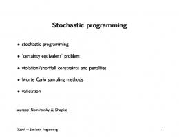
VALUE – AT – RISK & CONDITIONAL VALUE – AT – RISK EMPIRICS DISTRIBUTIONS

fb(X)

ab(X)

VALUE-AT-RISK & CONDITIONAL VALUE-AT-RISK EMPIRICS DISTRIBUTIONS jb( f(x) )

95% 5%

COSTS Mean

VaR

CVaR

jb( f(X) )

5% 95%

CVaR CVaR

VaR VaR

REVENUE Mean

CONDITIONAL VALUE – AT – RISK DISTRIBUCIONES EMPÍRICAS CVaR is commonly used in stochastic optimization models when we want to minimize the VaR or want to limit it. The basic equations included in the model are: fb(X) = ab(X) + (1-b)-1Sh=1,NE qh × wh

wh ≥ f(X|Yh) - ab(X) wh ≥ 0 where wh represents the excess loss over el VaR, ab(X) when occurs the scenario h.

The following expression is used to limit CVaR fb(X) ≤ CVaRMAX

G-SDDP – RISK MANAGEMENT CVAR – CONDITIONAL VALUE AT RISK Mean 387.094


459.503

307.566

Range 151.938

Frequency

Cost

G-SDDP – RISK MANAGEMENT CVAR – CONDITIONAL VALUE AT RISK Mean 387.094


459.503

307.566

Range 151.938

Frequency

MEAN RISK

MAXIMUM MINIMUM

Cost

G-SDDP – RISK MANAGEMENT CVAR – CONDITIONAL VALUE AT RISK Scenarios

Mean

100

387.09


459.50

307.57

151.94

Range

100

392.84

36.89

486.29

307.57

178.72

CVaR Limit Probability 444

0.05

VaR

CVaR

442.94

444

MIP EXPANSION: SOLUTION TIME VS. COMPLEXITY UNIFIED BENDERS CUTS – INEXACT SOLUTIONS

25000 TIME (sec)

Periods Scenario

20000

24 15000

Time/Scenario

1 5 10 20 100 200 400 800 1000 2000 4000

2.550 1.625 1.456 1.554 6.845 9.723 4.021 2.966 2.944 4.559 6.429

T. Solution (secs) 2.550 8.123 14.561 31.073 684.515 1944.649 1608.293 2372.763 2943.815 9118.668 25716.167

10000

5000

0 0

1000

2000

3000

4000

MIP EXPANSION: SOLUTION TIME VS. COMPLEXITY UNIFIED BENDERS CUTS – INEXACT SOLUTIONS

10.000

secs/scenario

7.500

Periods Scenario

5.000

24

2.500

1 5 10 20 100 200 400 800 1000 2000 4000

Time/Scenario 2.550 1.625 1.456 1.554 6.845 9.723 4.021 2.966 2.944 4.559 6.429

T. Solution (secs) 2.550 8.123 14.561 31.073 684.515 1944.649 1608.293 2372.763 2943.815 9118.668 25716.167

0.000 0

1000

2000

3000

4000

G-SDDP – LEARNING PROCESS

“The ordinate indicates the percentage proportion of each of the three groups of motor units relative to the total number of motor units M0(t) in the muscles: ▪ MA(t) motor units in activation; ▪ MF(t) motor units fatigued; ▪ Muc(t) motor units in the rest state. The time scale has been taken as arbitrary to show clearly the details and major features of the curves.”


6 5 4 3 2 1 0 0

MA(t)

Motor Units in Activation

2000

4000

6000

8000


MA(t)

Motor Units in Activation

G-SDDP: CONCLUSIONS

1. In all cases, the G-SDDP algorithm converge to optimal solution 2. G-SDDP approach is faster than SDDP 3. G-SDDP-UBC (one cut for all periods and stochastic scenarios) is faster than G-SDDP-ST (one cut for each period and each scenario). This fact justified efforts to manage the formulation with time independent matrices in the subproblems and to study the form to manage the solution of the problems when the costs of the control variables change are time dependent.

4. For the master problem, the integrated coordinator (IBC) is faster than the DDP coordinator. 5. Including inexact cuts in G-SDDP, in the case of MIP coordinators, speed up the velocity of the algorithm.

6. The relation between solution time and dimensionality of the stochastic problem is lineal, that implies that is possible to manage very large problems, in time and/or scenarios.

G-SDDP

COMMERCIAL IMPLEMENTATION

OPTEX MATHEMATICAL MODELING SYSTEM

IS A COMMERCIAL OPTIMIZATION TECHNOLOGY PRODUCED BY DO ANALYTICS (A SPIN OFF COMPANY OF DECISIONWARE)

(AVAILABLE IN SPANISH & ENGLISH)

FREE WEB-CONFERENCE 18/12/2017 18:00 UTC (00:00, Greenwich)

THE FIRST AUTOMATIC GENERATOR OF LARGE SCALE OPTIMIZATION MODELS “Civilization advances by extending the number of important operations which we can perform without thinking of them”. Alfred North Whitehead

Web-Conference Link: https://goo.gl/jA9LJV Slides OPTEX: https://goo.gl/Kpk9Q9

FREE WEB-CONFERENCE

18/12/2017

Hour 18:00 UTC (00:00, Greenwich)

THE FIRST AUTOMATIC GENERATOR OF LARGE SCALE OPTIMIZATION MODELS MODEL IN MS-WORD

ALGEBRAIC MODEL

PARÁMETROS Parámetro CTMItd CIFA td,tr FCTDud,td CIMIud,t d

CTVBud,td,tr

FILLING TABLES

CAMItd CALT td,tr

Descripción Costo de inversión de referencia mínimo si se instala un biodigestor con tecnología td Costo de inversión asociado al tramo tr si se instala un biodigestor con tecnología td Factor de ajuste de costos de inversión para la tecnología td en el sitio ud Costo de inversión de referencia mínimo si se instala un biodigestor con tecnología td en el sitio ud. Se calcula con base en la siguiente fórmula: CIMIud,t d = FCTDud,td × CTMItd Pendiente del tramo tr para el costo de inversión variable de un biodigestor con tecnología td en el sitio ud. Se calcula con base en la siguiente fórmula: CIVBud,td,tr = FCTDud,td × (CIFA td,tr+1 – CIFA td,tr ) / (CALT td,tr+1 – CALT td,tr ) Capacidad de procesamiento mínima de un biodigestor con tecnología td. Capacidad de procesamiento asociada al tramo tr para un biodigestor con tecnología td.

Uni dad

Tabla Referencia

Campo

$

MA E_TBD

CTMI

$

TBD_TCI

CIFA

UDB_TBD

FCTD

m 3-día

MA E_TBD

CA MI

m 3-día

TBD_TCI

CA LT

$

$/m 3día

LOAD EXCEL

.CSV FILES LOAD OPTEX

MODEL IN EXCEL CODE GENERATION INCLUDING LARGE SCALE METHODOLOGIES

OPL OPTIMIZATION TECHNOLOGY MODEL IN A COMPUTER LANGUAGE

GAMS Program generated by OPTEX to use G-SDDP

OPTEX - GAMS - G-SDDP

G-SDDP-UBC-CI-P CX: = { min z = S h=1,H S t=1,T h ( ct,hTxt + Wt,h ) | At xt,h = et,h "t=1,T "h=1,H t=1,T k T Wt,h + ( ) Et-1 xt-1 + (k)T At xt,h qt,hk "t=1,T "h=1,H "k=1,ISP } X = { xm1,h, xm2,h, … , xmT,H } Qt,hA = Wt,h(xt-1,h,xt,h) O(t)=f(Dz) LB = z

m = m+1

OPTIMIZATION DATA BASE Coordinator: xmt,h , LB Sub-Problem k , DZt,h , uk LU k=k+1 DZt,h

{ min z = dT u | B u = bt,h – E xt-1,h - A xt,h G u = gt,h uR+ }


k Qt,hB = dTu* = Qt,hB – Qt,hA


OPTEX – TYPES OF MODELS

INTEGRATED

Integrado (I): Modelo integrado por un solo problema. Corresponde a un modelo de optimización clásico. Valor por default para el tipo de modelo.

T-CHAIN

Encadenado Temporalmente (E): Define una cadena de problemas encadenados a lo largo del horizonte de planificación, se encadenarán de acuerdo con la secuencia que defina el usuario. Permite mezclar tipos de modelos a lo largo del tiempo. Por ejemplo, un modelo de MINLP para la primera semana y un modelo LP para las siguientes semanas. Se resuelve el problema integrado.

T-CHAIN-BEN Encadenado Temporal vía Benders: Igual a T-CHAIN, pero se resuelve el problema utilizando Teoría de Benders. R-LAGRANGE

Relajación Lagrangeana (R): Modelo cuyo coordinador es del tipo de Relajación Lagrangeana estándar.

SP-LAGRANGE Relajación Lagrangeana Estocástica (X): Modelo cuyo coordinador es del tipo de Relajación Lagrangeana Estocástica. El usuario debe indicar las variables que serán consideradas como noanticipativas. BENDERS

Benders (B): Modelo cuyo coordinador es del tipo de Benders Estándar, un coordinador y un subproblema. El sub-problemas deben ser un problema lineal; el coordinador puede ser lineal, mixto o no-lineal convexo.


DDP

Dual Dynamic Programming: Modelo dinámico que se resuelve siguiendo la metodología DDP (Dual Dynamic Programming, o Nested Benders). La DDP solo es aplicable a problemas lineales.

SDDP

Stochastic Dual Dynamic Programming: Modelo dinámico estocástico que se resuelve siguiendo la metodología DDP (Stochastic Dual Dynamic Programming). La SDDP solo es aplicable a problemas lineales.

GDDP-CU-CO

Generalized Dual Dynamic Programming: Modelo dinámico que se resuelve siguiendo la metodología GDDP (Generalized Dual Dynamic Programming). Para especificar el tipo de GDDP a utilizar se deben definir: 1. CU que especifica el tipo de corte, cuyos valores válidos son: ▪ CT Cortes desacoplados para cada período, por el sub-problema estático de cada período específico. ▪ C1 Cortes desacoplados para cada período, generados por un sub-problema estático que representa a todos los períodos. 2. CO que especifica la forma de resolver el coordinador, cuyos valores válidos son: ▪ CI: el coordinador se resuelve integrado ▪ CD: el coordinador se resuelve utilizando la metodología DDP. Los sub-problemas estáticos de la GDDP deben ser problemas lineales; el coordinador puede ser lineal, mixto o no-lineal convexo.

G-SDDP-CU-CO

Generalized Stochastic Dual Dynamic Programming: Modelo dinámico de optimización estocástica que se resuelve siguiendo la metodología G-SDDP (Generalized Stochastic Dual Dynamic Programming). Para especificar el tipo de G-SDDP se deben definir el tipo de corte y la forma de resolver el problema coordinador, se sigue la misma lógica que para la GDDP.


SP-PAR

Paralelo Estocástico (P): Define un conjunto de problemas que permiten analizar múltiples escenarios estudiados de forma paralela independientemente a cada escenario. No contiene restricciones de no-anticipatividad. Se resuelve cada problema de manera independiente.

G-SP-DDP-CU

Paralelo Estocástico GDDP: Define un conjunto de problemas que permiten analizar múltiples escenarios estudiados de forma paralela independientemente a cada escenario. No contiene restricciones de no-anticipatividad. Se resuelven todos los problemas conjuntamente, siguiendo los principios de la GDDP cada problema de manera independiente. Para especificar el tipo de G-SDDP se deben definir el tipo de corte y la forma de resolver el problema coordinador, se sigue la misma lógica que para la GDDP.

COOR-SEQ

Coordinador Secuencial (Q): Modelo con múltiples problemas los cuales serán resueltos secuencialmente de acuerdo con el orden que se especifique en el parámetro SEQ en la definición de los problemas.

COOR-SEQ-L

Coordinador Secuencial Loop (C): Modelo con múltiples problemas, donde la coordinación está definida por el usuario, similar al COOR-SEQ. Se resuelve cíclicamente hasta conseguir un determinado nivel de precisión, para ello el usuario define toda la conectividad y debe incluir en el modelo el parámetro GAP_FO el cual determina el proceso de parada, con base el error relativo del modelo definido como:

GAP_FO = | ( FO Estimación Dual – FO Valor Primal) | / | FO Estimación Dual |

OPCHAIN-E&G

IS A COMMERCIAL OPTIMIZATION SOFTWARE PRODUCED BY DECISIONWARE


OPCHAIN-E&G

MAKES USE OF G-SDDP MATHEMATICAL METHODOLOGIES & G-SDDP OPTIMIZATION TECHNOLOGIES


OPCHAIN-E&G

OPCHAIN-E&G-EDI Despacho Óptimo

OPCHAIN-E&G-NASH Despacho Óptimo Competitivo

OPCHAIN-E&G-SCD Optimización Diseño Red Generación

OPCHAIN-HID-SIN Generación Sintética MATALAS

OPCHAIN-E&G-MAN Optimización Mantenimiento

OPCHAIN-KALMAN Estimación de Estado DUAL KALMAN FILTER

COMMON

DATA MODEL

INFORMATION SYSTEM OPCHAIN-E&G-PSPOT Modelos Estadísticos ARIMA-GARCH

OPCHAIN-E&G-RDI Despacho Óptimo Regulado

OPCHAIN-E&G-ETRM Optimización Compra/Venta Electricidad

OPCHAIN-E&G-UC Optimización Operación Diaria

MATHEMATICAL MODELS OPCHAIN-E&G Model

OPCHAIN-E&G

EDI RDI

NASH UC FIN

SCD ETRM MAN

UC HID-SIM KALMAN PSPOT

Description DISPATCH SIMULATION IN POWER PLANTS The central model OPCHAIN-E&G corresponds to the clearance system generating plants which can be used by two types of agents for multiple purposes. Generically this model has been called OPCHAIN-E&G (Hydro-Thermal Simulation-Gas) and based on the same multiple models are built for specific purposes. The theoretical support of this model OPCHAIN-E&G gives rise to three variations of the model according to the economic concepts that support modeling. Economic (minimum cost): delivery of plants conventional office minimizes the cost of operation of the interconnected system Economic Regulated: Delivery of plants that minimizes the cost of operation of the interconnected system and includes representatives of regulatory aspects of the electricity market being simulated. Cournot-Nash equilibrium: Delyvery of plants oriented to the simulation of competitive electricity markets with agents that have the ability to influence their decisions on transactions occurring in the market. Unit Commitment associated with operational planning (short term) decisions related to delivery plants on a daily basis. Respect all non-linear constraints that are part of the delivery. Integrated simulation of economic dispatch plus financial modeling (ALM). Oriented to use in valuation of electric assets. UNIT STRATEGIC PLANIFICATION Associated with strategic planning (long-term) decisions related to designing the supply chain, in relation to capacity of reservoir, transfers, power plants and other elements of an electrical system. TACTICAL PLANIFICATION Energy Trading and Risk Management Oriented policy making preventive maintenance of multiple central generation plants. It can be applied to all plants in a region or a national grid. OPERATIVE PLANIFICATION Unit Commitment associated with operational planning (short term) decisions related to office plants on a daily basis. STOCHASTIC PROCESES MODELS Synthetic generation of water intake based on a model of Fiering-Matalas type. Projected short-term hydrological contributions via a Dual Kalman Filter Dual Projected electricity prices short-term competitive markets through ARMAX-GARCH models

OPCHAIN-E&G USER

MATHEMATICAL MODELER OPTIMIZATION TECHNOLOGY

OPTIMIZATION METHODOLOGIES

OPCHAIN-E&G USER


OPTIMIZATION METHODOLOGIES

OPL FINAL OPTIMIZATION TECHNOLOGY

TRANSPARENCY: ACCESS TO SOURCE CODE THE MATHEMATICAL MODELER CAN CHANGE, DELETE OR CREATE EQUATIONS OF THE MODELS, AND CAN CREATE NEW MODELS.

OPCHAIN-E&G USER


OPTIMIZATION METHODOLOGIES INTEGRATED OPL

LARGE SCALE:

FINAL OPTIMIZATION TECHNOLOGY

BENDERS THEORY GBD, DDP, GDDP, SDDP, G-SDDP

TRANSPARENCY: ACCESS TO SOURCE CODE

LAGRANGEAN RELAXATION

THE MATHEMATICAL MODELER CAN CHANGE, DELETE OR CREATE EQUATIONS OF THE MODELS, AND CAN CREATE NEW MODELS.

CROSS DECOMPOSITION

G-SDDP FUTURE RESEARCH & DEVELOPMENT

GENERALIZED DUAL DYNAMIC PROGRAMMING (GDDP)

DW-DOA are working in the implementation of the following methodologies G-NL-DDP Non-Linear Dual Dynamic Programming is the extension of the GDDP to the Non-Linear subproblems. G-DDiP Generalized Dual Dynamic Integer Programming is the extension of the GDDP to MIP subproblems. & the stochastics versions G-NL-SDDP & G-SDDiP

GDDP Extensions

FULL PROBLEM

BENDERS MASTER

BENDERS SUBPROBLEM

GDDP

NL-GDDP

GDDiP

NL-GDDiP

LP

LP

LP

YES

YES

YES

YES

MIP

NO

NO

YES

YES

NLP

NO

YES

NO

YES

MINLP

NO

NO

NO

?

MIP NLP

MINLP

LP MIP LP NLP LP MIP NLP MINLP

ASYNCHRONOUS PARALLEL OPTIMIZATION FOR MODELING MULTISECTOR INDUSTRIAL SYSTEMS (SUPPLY CHAINS)

An approach to solve large scale stochastic dynamic optimization problems using the combination of Multilevel Benders Decomposition and Lagrangian Relaxation. An analysis of how to establish families of problems in order to generate multiple cutting planes solving only one problem of the family (Unified Benders Cuts).

The families are related to zones, sectors, time, class of decisions (investments or operations), projects and/or stochastic conditions. A version of a parallel algorithm that uses a multiprocessor environment, where each processor is associated with one problem of the family.

MULTILEVEL BENDERS THEORY MinY f(Y) + Q(Y) Sujeto a:

F0 (Y) = b0 YeS

Q(Y) 

qkk (b - F(Y)) + zk (bz - Fz(Y))

k=1,NP

Z

Y

k

MinZ E Z + Qz(Z) Sujeto a:

Gz Z = bz - Fz(Y) Z e R+

q k k

MULTILEVEL BENDERS THEORY MinY f(Y) + Q(Y) Sujeto a:

F0 (Y) = b0 YeS

Q(Y) 

qkk (b - F(Y)) + zk (bz - Fz(Y))

k=1,NP

Z

Y

k

q k k

MinZ E Z + Qz(Z) Sujeto a:

Gz Z = bz - Fz(Y) Z e R+ h G Z + Qz(Z)  h (b - F(Y) )

h=1,NPX

h

Z Y MinX C X Sujeto a:

A X = b - F(Y) - G Z X e R+

INTEGRATED MODEL INVESTMENTS OPERATIONS INTEGRATED SYSTEM

INVESTMENTS

INVESTMENTS COORDINATOR

PARTITION

OPERATIONS

INTEGRATED OPERATIONS MODEL PARTITION INVESMENTS-OPERATIONS

PARTITION

INVESTMENTS


OPERATIONS

INTERSECTOR OPERATIONS COORDINATOR

SECTOR

MULTILEVEL SYSTEM

INTEGRATED OPERATION


SECTOR 1

SECTOR S DECOMPOSITION

PARTITION

INVESTMENTS


OPERATIONS

INTERSECTOR OPERATIONS COORDINATOR

SECTOR

ZONE

MULTILEVEL SYSTEM

INTERZONE COORDINATOR SECTOR 1

INTERZONE COORDINATOR SECTOR S





ZONE 1.1

ZONE 1.Z1

ZONE S.1

ZONE S.ZS

DECOMPOSITION

PARTITION

INVESTMENTS


OPERATIONS

INTERSECTOR OPERATIONS COORDINATOR INTERZONE COORDINATOR SECTOR 1

SECTOR


ZONE

DYNAMIC COORDINATOR ZONE 1.1

DYNAMIC COORDINATOR ZONA 1.Z1

DYNAMIC COORDINATOR ZONA S.1

TIME

1

1

1

MULTILEVEL SYSTEM

2

T-1

T

2

T-1

T

2

DECOMPOSITION

T-1

T

DYNAMIC COORDINATOR ZONA S.ZS

1

2

T-1

T

PARTITION

INVESTMENTS


OPERATIONS

INTERSECTOR OPERATIONS COORDINATOR INTERZONE COORDINATOR SECTOR 1

SECTOR

ZONE

DYNAMIC COORDINATOR ZONE 1.1


DYNAMIC COORDINATOR ZONA 1.Z1

DYNAMIC COORDINATOR ZONA S.1

DYNAMIC COORDINATOR ZONA S.ZS

GDDP TIME

MULTILEVEL SYSTEM

1

2

T-1

T

1

2

T-1

T

1

2

DECOMPOSITION

T-1

T

1

2

T-1

T

INVESTMENTS


PARTITION

RANDOM OPERATIONS

MULTILEVEL SYSTEM

MULTIPLE MODELS INTEGRATED UNDER DIFFERENT RANDOM CONDITIONS

DECOMPOSITION

INVESTMENTS

PARTITION

RANDOM OPERATIONS

MULTILEVEL SYSTEM


INTEGRATED OPERATIONS MODEL

INTEGRATED OPERATIONS MODEL

STOCHASTIC CONDITION 1

STOCHASTIC CONDITION H

DECOMPOSITION


INVESTMENTS

PARTITION

RANDOM OPERATIONS

SECTOR

ZONE

TIME

MULTILEVEL SYSTEM

INTERSECTOR OPERATIONS COORDINATOR STOCHASTIC CONDITION 1

INTERSECTOR OPERATIONS COORDINATOR STOCHASTIC CONDITION H

INTERZONE COORDINATOR SECTOR 1 STOCHASTIC 1

INTERZONE COORDINATOR SECTOR 1 STOCHASTIC H

DYNAMIC COORD. ZONE 1.1

DYNAMIC COORD. ZONA 1.Z1

1

1

2

T-1 T

2

T-1 T


G-SDDP DYNAMIC COORD. ZONA S.1

1

2 T-1 T

DYNAMIC COORD. ZONA S.ZS

1

2

T-1 T




DYNAMIC COORD. ZONA S.1

1

1

1

2

T-1 T

DECOMPOSITION

2

T-1 T

2 T-1 T


1

2

T-1 T


Joining the Decomposition Theory and the Partition Theory can be structured complex multilevel systems






1

2

T-1 T


1

2

T-1 T



1

2

T-1 T


1

2

T-1 T


1

2

T-1 T


1

2

T-1 T



1

2

T-1 T


1

2

T-1 T


These systems are characterized by the set of problem families that they include Each color represents a type of optimization problem





INTERZONE COORDINATOR SECTOR S STOCHASTIC 1

INTERZONE COORDINATOR SECTOR S STOCHASTIC H

related with a physical installation and/or decision level


1

2

T-1 T


1

2

T-1 T


1

2

T-1 T


1

2

T-1 T


1

2

T-1 T


1

2

T-1 T


1

2

T-1 T


1

2

T-1 T


Making a parallel with neural nets , the concept of problem family can be assimilated to a “neuron” class;






and the optimization process can be defined as a complex communications system between “neurons”

1

2

T-1 T


1

2

T-1 T

INTERZONE COORDINATOR SECTOR S STOCHASTIC 1


1

2

T-1 T


1

2

T-1 T


1

2

T-1 T


1

2

T-1 T

INTERZONE COORDINATOR SECTOR S STOCHASTIC H


1

2

T-1 T


1

2

T-1 T

STRUCTURE OF A SIMPLE ARTIFICIAL NEURON SOMA RESPONSE FUNCTION

X1

Xi X3 AXOM INPUT

W1,j Wi.j

S

Uj

W3,j DENDRITAS

AXOM INPUTS

SOMA (NUCLEO)

SYNAPSIS

AXOM OUTPUTS

Yj

AXOM OUTPUT

STRUCTURE OF A SMART ARTIFICIAL NEURON SOMA RESPONSE FUNCTION

X1

Xi X3 AXOM INPUT

W1,j

min dtTut | Wi.j Bt ut,h = bUt,h j - Et-1 xS t-1,h - At,hxt,h Gt.h ut,h = gt ut,hR+ } W3,j

DENDRITAS

AXOM INPUTS

SOMA (NUCLEO)

SYNAPSIS

AXOM OUTPUTS

Yj

AXOM OUTPUT


X1

Xi X3 AXOM INPUT

W1,j


DENDRITAS

AXOM INPUTS

SOMA (NUCLEO)

SYNAPSIS

AXOM OUTPUTS

Yj

AXOM OUTPUT


X1

Xi X3 AXOM INPUT

W1,j


Yj

AXOM OUTPUT

ASYNCHRONOUS PARALLEL OPTIMIZATION CX: = { min z = S h=1,H S t=1,T h ( ct,hTxt + Wt,h ) | At xt,h = et,h "t=1,T "h=1,H t=1,T k T Wt,h + ( ) Et-1 xt-1 + (k)T At xt,h qt,hk "t=1,T "h=1,H "k=1,ISP }

X = { xm1,h, xm2,h, … , xmT,H } Qt,hA = Wt,h(xt-1,h,xt,h) O(t)=f(Dz) LB = z

A COORDINATE WORK USING m = m+1 OPTIMIZATION TO SOLVE A MULTIPLE PROCESSORS DATA BASE LARGE SCALE OPTIMIZATION PROBLEM

BASED ON

BENDERS


Coordinator: xmt,h ,METHODOLOGIES LB LARGE SCALE LIKE: Sub-Problem k , DZt,h , uk LU THEORY, LAGRANGEAN RELAXATION k=k+1 & CROSS DECOMPOSITION.


DZt,h



PARALLEL OPTIMIZATION CX: = { min z = S h=1,H S t=1,T h ( ct,hTxt + Wt,h ) | At xt,h = et,h "t=1,T "h=1,H t=1,T k T Wt,h + ( ) Et-1 xt-1 + (k)T At xt,h qt,hk "t=1,T "h=1,H "k=1,ISP }


m = m+1






PARALLEL OPTIMIZATION CX: = { min z = S h=1,H S t=1,T h ( ct,hTxt + Wt,h ) | At xt,h = et,h "t=1,T "h=1,H t=1,T k T Wt,h + ( ) Et-1 xt-1 + (k)T At xt,h qt,hk "t=1,T "h=1,H "k=1,ISP }


m = m+1






REAL-TIME DISTRIBUTED OPTIMIZATION USING SMART METERING SYSTEMS (IoT)

REAL-TIME OPTIMIZATION USING STANDARD METERING SYSTEMS (SYNCHRONIZED)













Weeks Days Hours Time

MOMENTS IN WHICH RUN THE FULL OPTIMIZATION MODEL

REAL-TIME DISTRIBUTED OPTIMIZATION USING SMART METERING SYSTEMS (ASYNCHRONIZED) min dtTut | Bt ut,h = bt,h - Et-1 xt-1,h - At,hxt,h Gt.h ut,h = gt ut,hR+ }











Anytime

Time

MOMENTS IN WHICH RUN THE SUB-PROBLEMS MODELS EACH MODEL REPRESENT A PHYSICAL PRODUCTION SYSTEM


INTERSECTOR OPERATIONS STOCHASTIC COORDINATOR

INTERSECTOR OPERATIONS STOCHASTIC COORDINATOR

INTERZONE STOCHASTIC COORDINATOR

INTERZONE STOCHASTIC COORDINATOR

OPTIMIZATION

SECTOR 1

SECTOR 2

DATA BASE DYNAMIC COORD. ZONE 1.1


STATIC OPERATION S,Z,T,H

STATIC OPERATION STATIC OPERATION

S,Z,T,H

S,Z,T,H

"the computer-based mathematical modeling is the greatest invention of all times"

Herbert Simon Alfred Nobel Memorial Prize in Economic Sciences (1978) "for his pioneering research into the decision-making process within economic organizations

Herbert Alexander Simon (June 15, 1916 – February 9, 2001) was an American political scientist, economist, sociologist, psychologist, and computer scientist whose research ranged across the fields of cognitive psychology, cognitive science, computer science, public administration, economics, management, philosophy of science, sociology, and political science, unified by studies of decision-making. With almost a thousand highly cited publications, he was one of the most influential social scientists of the twentieth century. For many years he held the post of Richard King Mellon Professor at Carnegie Mellon University. Simon was among the pioneers of several of today's important scientific domains, including artificial intelligence, information processing, decision-making, problem-solving, organization theory, complex systems, and computer simulation of scientific discovery.

g-sddp generalized stochastic dual dynamic programming

g-sddp generalized stochastic dual dynamic programming

Suggest Documents

g-sddp generalized stochastic dual dynamic programming - Do Analytics

g-sddp generalized stochastic dual dynamic programming - Do Analytics

Analysis of stochastic dual dynamic programming method - H. Milton ...

On conditional cuts for Stochastic Dual Dynamic Programming

Primal and dual stochastic dynamic programming in ... - IEEE Xplore

Stochastic Dynamic Programming for Long Term

Discrete Stochastic Dynamic Programming (Wiley ... - Google Sites

Parallel Stochastic Dynamic Programming: Finite Element ... - CiteSeerX

Stochastic Dynamic Programming Using Optimal ... - Optimization Online

Optimal Reservoir Operation Using Stochastic Dynamic Programming

Application of Stochastic Dynamic Programming in ...

markov decision processes: discrete stochastic dynamic programming ...

Sampling Stochastic Dynamic Programming Applied to Reservoir ...

Stochastic equilibrium programming for dynamic ... - Springer Link

Dynamic Programming Approximations for a Stochastic ... - CiteSeerX

Approximate Stochastic Dynamic Programming for ... - Semantic Scholar

Dynamic Programming for Stochastic Target ... - Semantic Scholar

Stochastic Differential Dynamic Programming - Computer Science

Deterministic or stochastic dynamic programming? - AgEcon Search

Fuzzy Stochastic Dynamic Programming for Process ...

Stochastic Dynamic Programming Based Approaches to Sensor ...

Stochastic Dynamic Programming Based Approaches ...

Stochastic Programming

Stochastic programming