A. Pásztor
Simulacija grupiranja stvarne skupine robota ISSN 1330-3651 (Print), ISSN 1848-6339 (Online) UDC/UDK 004.896:004.942
GATHERING SIMULATION OF REAL ROBOT SWARM Attila Pásztor Original scientific paper This article deals with simulations of gathering problems using NXT robots. These robots are real mobile robots and gather synchronously, with no global navigation and communication and only limited visibility. In the first part I want to demonstrate that by increasing the capabilities of those robots that have poor communication and navigation abilities, they can be made suitable for simulating complex gathering methods. The gathering methods of robot swarms and robot teams have been an intensively investigated area of artificial intelligence. Several researchers have made theoretical algorithms for the solution of gathering problems but they have only used mathematical or robot simulators to test their ideas. In the second part the article discusses how after slightly modifying the Ando-algorithm and adapting it to real mobile robots, in the end, I could test the method not only with the help of mathematical simulator but also with real robots. Keywords: real NXT robot swarm, simulation of gathering methods, synchronous
Simulacija grupiranja stvarne skupine robota Izvorni znanstveni članak Rad se bavi simulacijom problema grupiranja pomoću NXT robota. To su stvarni pokretni roboti koji se grupiraju sinkrono, bez bilo kakve globalne navigacije i komunikacije te uz ograničenu vidljivost. U prvom dijelu želim pokazati da se povećanjem sposobnosti tih robota slabih mogućnosti komunikacije i navigacije, oni mogu osposobiti za simuliranje složenih metoda grupiranja. Metode grupiranja skupina robota i timova robota su područja umjetne inteligencije koja se intenzivno proučavaju. Nekoliko je istraživača sastavilo teoretske algoritme za rješavanje problema grupiranja no oni su koristili samo matematičke ili robotske simulatore za testiranje svojih ideja. U drugom se dijelu rada pokazuje kako sam, nakon neznatne modifikacije Ando-algoritma i prilagođavanja realnim pokretnim robotima, konačno uspio ispitati tu metodu ne samo uz pomoć matematičkog simulatora već i sa stvarnim robotima. Ključne riječi: simulacija metoda grupiranja, sinkroni, stvarna skupina NXT robota
1
Introduction
In the recent decades several academic researchers have investigated the behavioural patterns and habits of animals living freely in the nature and have tried to adapt the results of their observation to real robots. A relatively new field of artificial intelligence called "swarm intelligence" [1] is evolving. Some examples of swarm intelligence that can be observed in nature is the behaviour of ant colonies [2], the collective flying of bird swarms [3], the group movement of fish [4], the herd instinct of some mammals or the growth patterns of bacteria. One of the special areas of swarm intelligence tasks is when robots have to gather around an arbitrary point of an area or in a non-predetermined part of space. These procedures are usually called gathering methods. For testing the elaborated gathering procedures several researchers apply the intelligent agents' computerized simulation. For this purpose many people have used Webots mobile robot simulator [5], Repast general agent simulator [6], Microsoft Robotics Studio [7] or the Matlab program [8]. In most cases the simulated procedures are cost-effective and can help with the preliminary examination of the problem and the definition of the hypothesis. In my opinion the simulators, despite their numerous advantages, cannot replace experimentation with real robots, they can only supplement it. Several disturbing factors may arise during real experiments that we may ignore when we use only simulators to solve a problem. To examine the gathering process of robot swarm we have to define some basic characteristics of the robots involved. It should be determined whether the robots are Tehnički vjesnik 21, 5(2014), 1073-1080
represented by a point or they are fat robots, whether they can communicate with each other or not, if they use local or global navigation, if their visibility is limited or unlimited, whether they are transparent or not, and if they work synchronously or asynchronously. An important difference can also be whether the robots are oblivious or not, i.e. they do not remember any previous observation or computations performed in the previous steps. Most procedures distinguish three phases of the gathering process such as looking round, computing the new positions and moving into the new positions. One of the fundamental procedures among the gathering algorithms is the work of Ando et al. [9]. In their work they used point-like, oblivious and limited visibility robots which worked synchronous. The procedure applied the movement towards the centre of the smallest circle which can be pulled over the visible robots (SEC - Smallest Enclosing Circle) [22], but they took it into consideration that if two robots already see each other than visibility should never be interrupted between them. They proved the correctness of their local SEC algorithm in the synchronous case. Some researchers, such as Flocchini et al. [10] in their paper, presented a gathering algorithm (to be executed by each individual robot) which solves the problem within finite time. Their solution operates in fully asynchronous settings and can be achieved by robots which are anonymous, oblivious and have limited visibility. The robots were equipped with compass sensors and they used global localization. Cieliebak et al. [11] also adapted the SEC process and gave a solution to gathering problems where the robots were point-like, worked asynchronously, had no common coordination system, no identity, no central coordination, 1073
Gathering simulation of real robot swarm
no direct communication, no memory of the past, moving freely on the surface and were able to sense the positions of the other robots. Visibility was not unlimited. In their paper Bolla et al. [12] modified the Ando algorithm taking into consideration that real robots are disk-like, they are not transparent, they may collide and may block each other. In their work they proposed a solution to this problem, but instead of real robots MATLAB simulation was used for the demonstration of their hypotheses. Others, like Cohen and Peleg [13] instead of SEC used an algorithm based on centre of gravity, called COG. They used synchronous robots with unlimited visibility, arbitrary initial configuration. Degener et al. [14] proposed a solution for the synchronous limited visibility problem where instead of COG or SEC, their algorithm is based on the local convex hull of visible robots. In this process they have no global navigation but the robots can communicate with each other, since the robots can share their local coordinates and their moving strategy with each other. Klasing et al. [15] consider the problem of gathering identical, memoryless, point-like mobile robots in one node of a ring. Robots start from different nodes of the ring. They operate in Look-Compute-Move cycles and have to end up in the same node. In one cycle, a robot takes a snapshot of the current configuration, makes a decision to stay idle or to move to one of its adjacent nodes, and in the latter case, it makes an instantaneous move to this neighbour. Cycles are performed asynchronously for each robot. Czyzowicz et al. [16] used a robot with physical dimensions. The task was solved asynchronously and with no communication and just up to four robots. In the work of Chaudhuri and Mukhopadhyay [17] the robots have no memory either, move asynchronously and have physical dimension. It is assumed that the robots are completely transparent, on the other hand, and recognize the whole area. Furthermore, each robot has its perfect global navigation. In the proposed algorithm the problem of gathering was solved for at least five robots. In the research of Cord-Landwehr et al. [18] N mobile robots are collected around a given point as close together as possible so in this gathered state the space filling of the robots is optimal. The robots are disk-like (fat robots), do not use communication, have global navigation tools and total visibility, in this case it means that they are transparent. The robots move synchronous towards a central point unless they block each other. In those solutions where the robots are not point-like, of course, the robots cannot gather in a given point. In these methods it has to be determined when we consider the robot swarm gathered, for example, all the robots see all the others or the formation of the contact graph is coherent. In these cases another problem is that because of the fat robot representation the robots can collide so a robot could block the movement of another robot. This can be a deadlock situation so in the correct solution of task this possibility has to be taken into consideration.
1074
A. Pásztor
2
Synchronous gathering solution of NXT robot swarm using local navigation
In this article I use real, non-holonomic, programmable mobile robots to examine and simulate the robot swarms gathering problems. I would like to show that the various gathering simulations, like Andoalgorithm, are feasible with the help of NXT robots [19] in real and obstacle-free environment. In order to be able to use these robots in complex gathering solutions I have to increase the capabilities of robots due to poor communication and navigation abilities as described in the following sections. I had to reduce navigation inaccuracy resulting from inaccurate sensors, create local navigation, and define the exact rotation of robots without compass sensor or any other sensor and to avoid both collision and blocking during movement. Thus, while solving this problem an NXT robot swarm was scattered in an obstacle-free, arbitrary field and they had to gather and determine their own position using only odometry process and the rotation axis (robot rotation) calculation process. In the simulation the robots did not use direct communication channels (like Bluetooth, wireless sound or light based communication) and could only gain information from the position and movement of other robots. This is also called indirect communication. This can be easily seen in case of animals living at large, such as among fish. 2.1 Features of NXT robots used in the gathering simulation In my work I use real NXT mobile robots. The set of robots is denoted as R = {R1, R2,..Ri,…RN}. So that the robots could be used in gathering task, every single element of the robot swarm must have certain basic characteristics and abilities. NXT robots possess the most important characteristics or I have elaborated them with the help of the procedures described later. These main abilities are the following: Ability of autonom function: Ability of synchronous work: Collision-avoidance function: Memory and processor for computational operation: Visibility (limited): Ability of communication: Local localization:
NXT is able to work autonomously. with the help of sound sensor, sound generator, and inner time counter. with the usage of 3 distance sensors. 32 MB RAM, 256 KB FLASH memory,Atmel®32bit, ARM® AT91SAM7S256 processor. distance sensor (ultra sonic) there is only indirect communication, with the help of distance sensor. with the help of odometry method and "robot rotation count" method (described later)
Technical Gazette 21, 5(2014), 1073-1080
A. Pásztor
Simulacija grupiranja stvarne skupine robota
2.2 The odometry method and increasing local navigational accuracy In the cases when an area is completely unknown and no device can be connected to the robots that perceive the global external stimulus, namely, the robot has no global localization devices, for example compass sensor or GPS but if the robot has a certain capability, it is possible to use the odometry method. To use the method the robot has to have a step counter or, in the case the robot has wheels, it has to have a counter of wheel rotation axes called tachograph. The essence of the method is that the robot counts the wheel rotations from the starting point and counts axle rotations too (robot axle rotation counter method is described in the next chapter), so it can define its actual position compared to the starting position. The NXT robots possess these abilities; they have an interactive wheel which can count their own rotation. The definition of the current positions of the robots happens with the help of the under mentioned simple formula (1). In the formula the axis length (distance between the two wheels) is denoted as t, the travelled distance of the right wheel as Δsj, the left wheel as Δsb, the Cartesian coordinates of starting point as x and y, the directional angle of rotation as ϕ and the current position as x’, y’. This formula can be used to estimate the new odometric position of the robot.
Δsj + Δsb Δsj + Δsb ⋅ cos φ + 2 2 t x ' x y' = y + Δsj + Δsb ⋅ sin φ + Δsj + Δsb . 2 2t φ' φ + Δ Δ sj sb t
accuracy is greatly degraded when rotation is imprecise. To determine the robot rotation angle accurately several researchers use a compass sensor but in the simulation I wanted to use just local positioning devices, therefore the robot rotation angles were determined by a simple mathematical method. If the radius of robot wheel, the length of the horizontal axis (distance of two wheels) and the angle of wheel rotation are known, the rotation angle of robot (virtually, the axial rotation angle which connects the two wheels) can be simply determined (in Fig. 1).
(1)
The programs which are necessary to control the NXT robots are written in NXC programming language and in Bricx Command Centre 3.3.17 programming environment [20] and the 1.03 firmware is run on the robots. In the simulation for the localization of robots only the local navigation system was applied so I could only use the odometry method but this can often be inaccurate because of the roughness of the ground, the different size of wheels or the improper load-distribution. In order to achieve more accurate navigation I applied the wheel-synchronization (OnFwdSyncr() ) function of controller language, furthermore, the intelligent wheels of the robot have a rotation counter and with the help of it the distance done by the robot can be calculated. In the interest of accuracy I used calibration, too. I did dozens of experiments and measurements and I managed to reach 1,4∗E-2 navigation accuracy on a 6-meter distance [21]. Using compasses built upon the robots I could reach greater accuracy (3,0∗E-3), but in my gathering simulation I did not use global navigation devices. 2.3 Determining the rotation angle of robots
Figure 1 Determining the rotation angle of robots
It can be clearly seen from the derivation (2) that knowing the rotation angle of wheels, the rate of stub axis and the radius of wheels, the rotation angle of the robot can be simply determined. π π , = φ ⋅t ⋅ 180 180 λ ⋅ r ⋅ π 180 λ ⋅ r , ⋅ = φ= 180 t ⋅ π t s = λ ⋅r ⋅
(2)
where: s − length of the route covered by the wheel, r − radius of wheel, t − length of stub axle, λ − rotation angle of wheel and φ − rotation angle of robot (axial). In the robot control program these data are at the disposal of the robot or can be calculated from the function of NXC programming language. (MotorRotationCount()). In the concrete program it means that 4° rotation angle of wheel causes 1° rotation angle of robot (axial).
During the gathering simulation the robots move not only in a straight line but they also have to execute some rotation with different angles. Of course, robot navigation Tehnički vjesnik 21, 5(2014), 1073-1080
1075
Gathering simulation of real robot swarm
2.4 Defining the positions of visible robots with distance sensor Since the robots do not communicate with each other, they cannot send information on their positions to the other robots. However, in order to gather the robots, it is necessary for each robot to determine the positions of the other robots related to them. An ultrasonic sensor is used to define the distances between two robots which, according to the data of the manufacturing factory, reflect the distances exactly up to 254 cm. I tested these sensors for 60 – 120 – 150 – 200 – 250 cm and the measured results clearly show that these sensors are reliable and mistakes up to 2 m (1 ÷ 3 cm) occur relatively rarely. Many times the sensor did not notice the objects which were farther than two meters so in my simulation I supposed that the range of maximum visibility of robots is 2 m. I tested whether it would cause any interference or a measurement error if several robots got near each other but the results of measurements show that several robots can safely measure distances simultaneously. Fig. 2 shows that after two laps the measuring robot determined the same distances and angles.
A. Pásztor
2.5 Avoiding collisions and deadlock situations As the robots are not point-like and have 3 dimensions (22 × 18 × 14 cm), collision avoidance must be resolved during their movement. With the help of its three distance sensors a robot can perceive an angle of 160° in front of itself. In this case, if another robot crosses its path and the distance between the two robots is less than 30 cm, the robots stop. Unblocking the resulting deadlock situation is described in the phases of simulation part in more detail. 3
The phases of simulation
The basis for my simulation is the Ando-algorithm [9] whose correctness is proven for point-like robots. During the execution of synchronous algorithms the gathering tasks are divided into three main phases. The beginning of the simulation is a 1 kHz sound signal so the robot must be supplied with a sound sensor to perceive the sound signals. Additionally, each robot is equipped with three distance sensors, in the case of NXT it is called Ultrasonic Sensor (in Fig. 4). The middle sensor measures the distance of the robot from the others and the two other sensors are used to avoid collision during the movement.
Figure 4 NXT robot used in the simulation
Figure 2 The result of testing the distance sensor. The numbers on the picture mean the number of visible robots
Thus, if any Ri robot position is considered P (0, 0) point, its longitudinal axis is axis Y and the latitude axis is axis X then any Rj robot position that is within the visibility can be determined (compared to Ri) with the help of the middle ultrasonic sensor and the procedures of determining the rotation angle described in the previous section (in Fig. 3).
In the first phase the robots turn around and determine the positions of those robots which are within the visibility distance and are not covered by other robots. This phase is called "Look around". In this phase all the robots turn 360° with the help of the "Determining the rotation angle" procedure (in Section 2.3) and save the positions of robots which are within the visibility circle. This distance is maximum 2 m. There can be some robots - denoted Rk in Fig. 5 which are outside the visibility circle of Ri. If the distance of a robot from any other robot is more than 2 m, it does not take part in the simulation. In the second phase of gathering the robots with the help of the determined positions of other robots and based on their own position calculate the centre of the smallest circle (SEC) which can be drawn around the visible robots. It is denoted Pi (in Fig. 5). This phase is called "Calculate new positions". All robots do this calculation simultaneously but the different robots can see different companion robots so the new goal positions of different robots can be different. They turn in this new direction and start moving towards the calculated centre of the "smallest circle".
Figure3 Determining the position of Rj robot (compared to Ri) 1076
Technical Gazette 21, 5(2014), 1073-1080
A. Pásztor
Simulacija grupiranja stvarne skupine robota
during the moving phase. So the real length of moving Ri is calculated in Eq. (4). R i movelength = min ( length(Ri,Pi), min(sj)).
Figure 5 Calculate new positions
Ando had two things on his mind in his proven algorithm. The first viewpoint is to let the robots try to approach each other. The other viewpoint is, if two robots can see each other at time T, then they must see each other at time T+1, too. Therefore, after calculating the centre of the smallest enclosing circles the robots do a new calculation before starting again. This is necessary so as not to break the visibility graph which has already been formed. Each robot examines this separately in the case of each visible robot member of the swarm. Let’s examine two robots denoted Ri and Rj that can see each other at time T. If we want these two robots to see each other at time T+1, then Ri during its moving must not leave the dashed circle denoted Cj (in Fig. 6).
Figure 6 Calculate the move length of Ri
(4)
In the third phase of the simulation the robots move to the previously calculated new positions. It is called "Moving phase". In this part each robot turns towards the calculated direction and covers the previously described length. The first synchronization signal at the beginning of the simulation is a 1 kHz void signal but the others are generated by the robots own Timer() function for the different phases. Because the robots have extension (22 × 18 × 14 cm), during this phase the collision avoidance procedure is run by the robots. In the Ando-algorithm the robots are point-like so there is no collision or blocking, but because of using real robots the algorithm has been modified. With the help of three distance sensors the robot perceives an angle of 160° in front of itself. In this case, if Ri and Rj robots cross each other's path and the distance between the two robots is decreased to 30 cm, the robots stop. In this phase they do not move. If in the special case only robot Ri can see the back part of Rj (there are no sensors) then Ri stops and Rj can move onward. Unblocking the resulted deadlock situation is illustrated in Fig. 7a. In the "Look around" phase Ri saves the position of Rj if it is closer than 30 cm. Then robot Ri calculates the new positions denoted PRi. Because of the deadlock situation PRi is modified. The modified P’Ri is on the tangential of Ri safety circuit and the length of the new PRi goal vector is calculated as the projection of the original PRi goal vector to the tangential direction.
Figure 7 Avoiding the deadlock situation
The centre of this circle denoted mj is the midpoint of the straight segment joining robots Ri and Rj, and its radius is L/2 (1 m in the simulation), this is half of the visibility distance. The distance between Ri and Rj is denoted dj. This assumption is true as well in the case of Ri. Under these conditions the edges of visibility graph do not break, it can be simply demonstrated by basic geometrical methods (in Fig. 6). Let sj denote this distance which Ri can cover in the case of Rj and it can be calculated with the following formula (Eq. 3):
In the new "moving phase" Ri first turns in the opposite direction to Rj and moves forward to the tangential of Ri (30 cm) then it turns in the direction of P’Ri and starts to move towards this point (in Fig. 7b). In the case when three or more robots cross each other's path those robots which meet more than one robot remain in place in the next phase but those which have only one crossing neighbour move onward.
s j = (d j /2)cos α j + ( L / 2) 2 − ((d j /2) 2 (sinα j ) 2 .
After this the phases of the simulation cyclically repeat till the completion of the task. The end of the task can be defined in several ways. Since the robots are not point-like they cannot gather even theoretically in one point. We may regard the task finished when a predefined beginning condition is fulfilled. Such stop condition may
(3)
Robot Ri has to calculate this sj distance for each Rj robot located in the visibility circle of Ri and then has to find the minimum of sj. It is the most stringent limit Tehnički vjesnik 21, 5(2014), 1073-1080
3.1 The end of simulation
1077
Gathering simulation of real robot swarm
be if the robots are no longer able to move or a related contact graph is formed (Fig. 8). In my simulation it means that the security zone of each robot is in contact with at least another robot and from any robot which is the element of the contact graph any other robot is available through the nodes of the graph.
Figure 8 The contact graph is formed
A. Pásztor
temporarily I wanted to prove only that with the NXT robots the modified algorithm is feasible. The robots are situated on the peaks of a two-meter longitudinal side of a regular triangle (Fig. 9a), then of a regular hexagon (Fig. 9b) and, finally, of a decagon (Fig. 9c). In the first case two steps, in the second case three steps and in the third case five steps were necessary for the robots to create the contact graphs. I conditioned these step numbers in the real robot simulation. After the Matlab simulation I run the readymade program on the NXT robots as described above. In the first simulation when three robots were used the result of the simulation was similar to the Matlab one. On the upper part of the picture can be seen the starting positions of three robots and on the bottom the gathered robots (Fig. 10).
The gathering may end after a given time limit or achieve the specified number of successive phases. 4
Results
In the previous sections I have described some procedures for real NXT robots so with their help the gathering algorithm can be realized. Before testing my gathering algorithm, which is a modified Ando-algorithm (collision avoidance, unblocking deadlock situations), we tested it with the help of Matlab program, too.
Figure 10 The starting and gathered positions of the robot swarm
Figure 9 The results of the gathering simulation using Matlab. The left pictures show the starting positions and the right pictures the positions of robots at the end of simulation.
In the tests R =3, 6, 10 robots were used. In this case, the starting positions of the robots are special cases, 1078
In the second robot simulation when I used six robots the robots are gathered closer together but the calculated positions in Matlab were slightly different from the expected positions. The robot which is denoted in the picture by a circle arrived but not punctually to its calculated place but the contact graph is formed (Fig. 11). In the third case I used ten robots. In the second cycle the denoted robot because of the possible error of the odometry method differed from the calculated direction significantly so the next step its neighbour on the left calculated a different direction from the theoretical waited direction, too. The theoretical direction is denoted by a red arrow. Nevertheless, at the end of the gathering procedure the robots were gathered and the contact graph was created. It can be seen clearly in the picture that this graph is different from the calculated one in Matlab (Fig. 12).
Technical Gazette 21, 5(2014), 1073-1080
A. Pásztor
Simulacija grupiranja stvarne skupine robota
are gathered closer together but the calculated positions were slightly different from the expected positions. It can happen due to the errors of the sensors and the rounding inaccuracy of the calculation procedure and the odometry method. In the future I would like to use an infrared distance sensor called IRSeeker, it is more accurate, can be used on longer distances and its viewing angle is 240° which enhances collision avoidance as well. I would like to use a gyroscope sensor to measure the turning of robots more accurately. I want to test my algorithm on the modified robots with at least twenty robots not only in special cases but in general ones as well. Acknowledgements
Figure 11 The simulation with six robots
This research was supported by the European Union and the State of Hungary, co-financed by the European Social Fund within the framework of TÁMOP 4.2.4.A/2-11-1-2012-0001 "National Excellence Program". I would like to thank Kálmán Bolla who helped me very much in the Matlab simulation. 6
Figure 12 The gathering method with ten robots. The theoretically calculated direction is denoted by a red arrow.
5
Conclusions and future plans
In my work I have shown how to develop the capabilities of NXT robots so that they would be suitable to simulate complex gathering methods. I have increased the ability of robots to enable them to run and carry out this modified Ando-algorithm and at the end of the simulation they could form a contact graph at least in special cases. I made the simulation in special cases where 3, 6, 10 robots were used and their starting positions were on the peaks of regular polygons and a robot could see only its two neighbour robots. The robots Tehnički vjesnik 21, 5(2014), 1073-1080
References
[1] Beni, G.; Wang, J. Swarm Intelligence in Cellular Robotic Systems, Proceed. NATO Advanced Workshop on Robots and Biological Systems, Tuscany, Italy, 1989. [2] Dorigo, M. ed. Ant Colony Optimization and Swarm Intelligence, 5th International Workshop, ANTS 2006, Brussels, Belgium, September 4-7, 2006, Proceedings. Vol. 4150. Springer, 2006. [3] Kushleyev, A. et al. Towards a swarm of agile micro quadrotors. // Autonomous Robots. 35, 4(2013), pp. 287300. [4] Xiao-Lei, Li; Shao, Zhi-jiang; Qian, Ji-Xin. An optimizing method based on autonomous animats: fish-swarm algorithm. // System Engineering Theory and Practice. 22, (2002), pp. 32-38. [5] Michel, O. Webots: a powerful realistic mobile robots simulator. // Proceeding of the Second International Workshop on RoboCup. Springer-Verlag, 1998. [6] Collier, N.; Howe, T.; North, M. Onward and upward: The transition to Repast 2.0. // Proceedings of the First Annual North American Association for Computational Social and Organizational Science Conference, 2003. [7] Jared, J. Microsoft robotics studio: A technical introduction. // Robotics & Automation Magazine, IEEE 14.4, 2007, pp. 82-87. [8] Hanselman, C. Duane and B. Littlefield. Mastering Matlab 7. Pearson/Prentice Hall, 2005. [9] Ando, H.; Suzuki, I.; Yamashita, M. Formation and Agreement Problems for Synchronous Mobile Robots with Limited Visibility, Symposium of Intelligent Control, 1995, pp. 453-460. [10] Flocchini, P.; Prencipeb, G.; Santoroc, N.; Widmayer, P. Gathering of asynchronous robots with limited visibility. // Theoretical Computer Science. 2005, pp. 147-168. [11] Cieliebak, M.; Flocchini, P.; Prencipe, G.; Santoro, N. Solving the Robots Gathering Problem. ICALP 2003. LNCS, vol. 2719. Springer, Heidelberg, 2003, pp. 11811196. [12] Bolla, K.; Kovacs, T.; Fazekas, G. Gathering of fat robots with limited visibility and without global navigation. // Swarm and Evolutionary Computation, Springer Berlin Heidelberg, 2012, pp. 30-38. 1079
Gathering simulation of real robot swarm
A. Pásztor
[13] Cohen, R.; Peleg, D. Local Spread Algorithms for Autonomous Robot Systems. // Theoretical Computer Science. 399, (2008), pp.71-82. [14] Degener, B.; Kempkes, B. A local O (n2) gathering algorithm. // Proceedings of the 22nd ACM symposium on Parallelism in algorithms and architectures. ACM, 2010. [15] Klasing, R.; Markou, E.; Pelc, A. Gathering asynchronous oblivious mobile robots in a ring. // Theoretical Computer Science. 390, (2008), pp. 27-39. [16] Czyzowicz, G.; Gasieniec, L.; Pelc, A. Gathering few fat mobile robots in the plane. // Theoretical Computer Science. 410, (2009), pp. 481-499. [17] Chaudhuri, G.; Mukhopadhyaya, K. Gathering Asynchronous Transparent Fat Robots, ICDCIT 2010. LNCS, vol. 5966, Springer, Heidelberg, 2010, pp. 170-175. [18] Cord-Landwehr, et al. Collision less Gathering of Robots with an Extent. SOFSEM 2011. LNCS, vol. 6543, Springer, Heidelberg, 2011, pp. 178-189. [19] Lego MINDSTORMS NXT. URL: http://en.wikipedia.org/ wiki/Lego_Mindstorms_NXT [20] Benedettelli, D. Programming legonxt robots using nxc, URL: http://bricxcc.sourceforge.net/nbc/nxcdoc/ NXC_Guide.pdf [21] Pásztor, A.; Kovács, T.; Istenes, Z. Compass and Odometry Based Navigation of a Mobile Robot Swarm Equipped by Bluetooth Communication, ICCC CONTI 2010, IEEE International Joint Conferences on Computational Cybernetics and Technical Informatics, Timosoara, Romania, 2010, pp. 565-570. [22] Elzinga, D. J.; Hearn, D. W. Geometrical solutions for some minimax location problems. // Transportation Science. 6, (1972), pp. 379-394. Author’s address Attila Pásztor, Dr. Associate Professor Kecskemét College Faculty of GAMF 6000 Kecskemét, Izsáki str. 10 Hungary E-mail:
[email protected]
1080
Technical Gazette 21, 5(2014), 1073-1080