Dec 13, 2013 ... problems in pathology slides of human tissue. The first is image ... stained
cardiomyopathy slides, our classes are the foreground cells (ie.
Gaussian Process Based Image Segmentation and Object Detection in Pathology Slides CS 229 Final Project, Autumn 2013
Jenny Hong Email:
[email protected] I.
I NTRODUCTION
In medical imaging, recognizing and classifying different cell types is of clinical importance. However, this requires a medical expert to perform the arduous task of manually annotating images. Therefore, we seek to better automate the two following problems in pathology slides of human tissue. The first is image segmentation, or categorizing pixels into labeled classes. For our dataset of H&E stained cardiomyopathy slides, our classes are the foreground cells (ie. cardiomyocytes), ”background” cells in the interstitial space, and nuclei in either region. The second problem is object detection, or identifying instances of some class. In this case, our primary interest is identifying instances of cardiomyocyte cells. This greatly aids in medical annotations and allows experts to focus on annotating only the interstitial cells, which are the parts that most require expert attention to label. We extend existing methods for object detection by proposing a new model for shapes of objects. For each cell, we develop a radial representation, which we call a shape profile. We then learn Gaussian processes from these profiles model the prior distribution over shapes. Such a model is relatively new in the literature [5] and the work has not also combined this technique with the process of proposing new boundaries for cells in a generative method. We then further augment this method by building off of existing methods for seed detection, which is important for refining the radial representations.
0 200 400 600 800 1000 1200 1400 0
Fig. 1.
500
1000
1500
Original H&E Stained Slide with bounding boxes
This project is an extension of Jenny’s work under David A. Knowles during Stanford CS Undergraduate Research Internship during the summer of 2013, where she developed the image segmentation portion of the project and began initial work on the shape profile model for Gaussian processes. December 13, 2013 II.
M ETHODS
A. Image Segmentation For multi-label segmentation, we use the approximate graph cuts-based algorithm proposed by Boykov et al. [2], minimizing energies of the form E(f ) =
X {p,q}∈N
Vp,q (fp , fq ) +
X p∈P
Dp (fp )
(1)
0
0
200
200
400
400
600
600
800
800
1000
1000
1200
1200
1400 0
Fig. 2.
500
1000
1500
Results of Image Segmentation
where N is a set of four-connected neighboring pixels and P is the set of pixels. The potentials respectively seek smoothness (ie. similarity of neighboring pixels) and fidelity to the original image. For each class, to calculate the unary potentials, we learn a Gausian mixture model with pixels as individual data points. Each pixel is represented by a vector consisting of its RGB values in the original image.
1400 0
Fig. 3.
500
1000
1500
Results of Connected Component Labeling
B. Object Detection Our goal in this stage is to identify components with smooth outlines, so that we can generate shape profiles as described in the next section. Starting with the segmentation generated from the previous step, we reduce the image into binary background vs. non-background classes and use a simple flood fill algorithm to identify connected components of the same class. Fig. 3 shows the results of connected component labeling (each color represents a different connected component).
A small set of hand-labeled pixels (relative to the image size), serves as the training data for the Gaussian mixture model. We have labeled two bounding boxes of pixels per class, to simulate the type and amount of data a human would provide if labeling an image in an interactive environment. An example image with bounding boxes (in green) is shown in Fig. 1.
For each object, we construct a shape profile, or radial representation, by measuring the radius from the center at 20 evenly spaced angles from 0 to 2π. The initial guess of the center is taken to be the centroid of all pixels assigned to the given connected component. However, later iterations can incorporate the centers found by the seed detection component of the project.
For the pairwise potentials, we started with potentials of larger magnitude from a class to itself, which promotes identifying coherent, connected objects. We also gave small potentials to cardiomyocyte and background, and cardiomyocyte and nucleus.
This representation allows us to represent a shape with fidelity to the exact pixels used in the shape but in a very compact way. From these shapes, we learn parameters to represent a prior distribution over the shapes via a Gaussian process. For our covariance function, we use the following periodic random function [4] over x
The result of the image segmentation process is shown in Fig. 2
k(x1 , x2 ) = A exp(−
sin2 (|x1 − x2 |) ) 2l2
(2)
Fig. 4.
50 45 40 35 30 25 20 150
1
2
3
4
5
6
60 50 40 30 20 10 00
1
2
3
4
5
6
Sample Gaussian Process Parameters
A is the amplitude and learns the average radius or measure of size for each cell. l is the lengthscale, or strength of correlation between two points as a function of their distance. For example, l can distinguish between an elliptical cell shape, such as the ground truth cardiomyocyte labeling, a figureeight cell, such as two cells incorrectly identified as one connected component. We found the parameters to be influenced very little by the prior distributions given over their values. However, they were strongly influencedqby N initial values. We used initial values A0 = π where N is the number of pixels in the connected component and a small constant for l0 . Fig. 4 shows a shape profile and the parameters of the Gaussian process learned from it. The dashed green line represents the mean and the shaded gray area extends to one standard deviation above and below. C. Seed Detection The Gaussian process technique learns parameters over the prior distribution of shapes, but it does not directly aid in identifying the centers or, more importantly, the boundaries of these shapes. Identifying accurate centers is important in finding a shape profile with high fidelity, and to that end, we use a multiscale Laplacian of Gaussian filtering
Fig. 5.
Laplacian of Gaussian filter with σ = 10
method proposed by Al-Kofahi et al. [1]. The multiscale LoG method originally used an exact binary graph-cuts algorithm to classify foreground and background for pre-processing. However, because of richer image data and different needs, we have binarized our image after a multilabel segmentation via flood fill. The multiscale LoG method simultaneously gives estimates of the shape and of the center for each cell. The scale-normalized LoG filter is given by ∂ 2 G(x, y; σ) ∂ 2 G(x, y; σ) + ) ∂x2 ∂y 2 (3) where σ is the scale value and G(x, y; σ) is a Gaussian with 0 mean and scale σ.
LoGnorm (x, y; σ) = σ 2 (
Fig. 5 shows the LoG filter detecting centers well for the given σ. In particular, red areas show pixels that are good fits of centers whose borders align with the filter. The centers of cells in the image are given by peaks in the response surface RN (x, y) = argmaxσ {LoGnorm (x, y; σ) ∗ IN (x, y)} (4) For each connected component C where C is a set of pixels, the estimate of its center is therefore given by argmax(x,y)∈C RN (x, y). This is again a modification of Al-Kofahi et al.’s method, which
Veta of the Image Sciences Institute [7], a ground truth data set. We also plan to data from the UCSB Bio-Segmentation Benchmark dataset [3], also H&E stained breast cancer images. III.
Fig. 6.
Sample centers detected by the Laplacian of Gaussian filter
used watershed flooding to detect all local maxima rather than restricting to one per connected component. This method allows us to choose exactly one center per connected component to generate the shape profile for the Gaussian process part of the object detection process. It also simplifies the problem by allowing us to use the Guassian process to focus only on under-segmentation (ie. when two or more ground truth cells are detected as one connected component) instead of also addressing over-segmentation, which was not a problem for our data set. However, this means we must rely entirely on the score assigned by the Gaussian processes to detect when we should split components. In the original method, the multiscale LoG method implicitly contributed to detecting places to split, because each local maximum indicated one cell. D. Data Set Thus far, we have run our methods on transverse and longitudinal H&E stained cardiomyopathy slides provided by Andrew Connolly of the Stanford Medical School. (Figures in this paper are taken from tranverse slides.) For comparative analysis, we plan to test further using result from H&E stained breast cancer histopathology images from Mitko
C ONCLUSION
In this project, we have explored the effects of two approaches to object detection that run in parallel: Gaussian processes based on shape profiles and multiscale Laplacian of Gaussian filters. Each method gives an independent estimate of two values: (1) the size of the cell (corresponding to a parameter of the Gaussian process and the scale of the LoG filter) and (2) the fit of a connected component (corresponding to the score assigned to a component by the Gaussian process and whether the original multiscale LoG filtering method by Al-Kofahi et al. yields multiple seeds per connected omponent). The main goal of immediately further work is to integrate these two estimates iteratively. That is, a proposed workflow is to iterate between the Gaussian process method and the multiscale LoG method instead of running them in parallel. After one method completes, its estimates of the two values above can be passed to the second one, such as in the form of prior beliefs of the values. We thus aim to build an integrated method with better performance than either method individually. Finally, we plan to integrate these techniques into the Interactive Learning and Segmentation Toolkit (ilastik) [6]. ACKNOWLEDGMENT This project was advised by David A. Knowles, postdoctoral researcher at Stanford University. In the in the initial segmentation process, we use Andrew Mueller’s pygco library, which is a Python wrapper for Boykov’s implementation of his multi-label graph cuts method in C++. Our implementation of the Gaussian process builds off of the open source PYGP Gaussian process toolbox for Python. The author would also like to thank Andrew Connolly and Mitko Veta for personally providing their H&E slides for use in our data set.
R EFERENCES [1]
[2]
[3]
[4] [5]
[6]
[7]
Y. Al-Kofahi, W. Lassoued, W. Lee, and B. Roysam. Improved Automatic Detection and Segmentation of Cell Nuclei in Histopathology Images. IEEE Transactions on Biomedical Engineering, 57(4):841–852, April 2010. Y. Boykov, O. Veksler, and R. Zabih. Fast Approximate Energy Minimization via Graph Cuts. IEEE Transactions on Pattern Analysis and Machine Intelligence, 23(11):1222–1238, November 2001. E. D. Gelasca, J. Byun, B. Obara, and B. Manjunath. Evaluation and benchmark for biological image segmentation. In IEEE International Conference on Image Processing, Oct 2008. C. E. Rasmussen and C. K. I. Williams. Gaussian Processes for Machine Learning. The MIT Press, 2005. T. Shepherd, S. J. Prince, and D. C. Alexander. Interactive lesion segmentation with shape priors from offline and online learning. Medical Imaging, IEEE Transactions on, 31(9):1698– 1712, 2012. C. Sommer, C. Straehle, U. Koethe, and F. A. Hamprecht. ”ilastik: Interactive learning and segmentation toolkit”. In 8th IEEE International Symposium on Biomedical Imaging (ISBI 2011), 2011. M. Veta, P. J. van Diest, R. Kornegoor, A. Huisman, M. A. Viergever, and J. P. W. Pluim. Automatic Nuclei Segmentation in H&E Stained Breast Cancer Histopathology Images. PLoS ONE, 8, 2013.