Sep 14, 2016 - We refer to our approach as âgray-boxâ inference since, in principle, for general ...... Aaron Defazio, Francis Bach, and Simon Lacoste-Julien.
Gray-box inference for structured Gaussian process models Pietro Galliani1 , Amir Dezfouli2 , Edwin V. Bonilla3 , and Novi Quadrianto1
arXiv:1609.04289v1 [stat.ML] 14 Sep 2016
1
SMiLe CLiNiC, University of Sussex, Brighton, UK 2 Data61, CSIRO, Sydney, Australia 3 The University of New South Wales, Sydney, Australia September 15, 2016 Abstract We develop an automated variational inference method for Bayesian structured prediction problems with Gaussian process (gp) priors and linear-chain likelihoods. Our approach does not need to know the details of the structured likelihood model and can scale up to a large number of observations. Furthermore, we show that the required expected likelihood term and its gradients in the variational objective (ELBO) can be estimated efficiently by using expectations over very low-dimensional Gaussian distributions. Optimization of the ELBO is fully parallelizable over sequences and amenable to stochastic optimization, which we use along with control variate techniques and state-of-the-art incremental optimization to make our framework useful in practice. Results on a set of natural language processing tasks show that our method can be as good as (and sometimes better than) hard-coded approaches including svm-struct and crfs, and overcomes the scalability limitations of previous inference algorithms based on sampling. Overall, this is a fundamental step to developing automated inference methods for Bayesian structured prediction.
1
Introduction
Developing automated inference methods for complex probabilistic models has become arguably one of the most exciting areas of research in machine learning, with notable examples in the probabilistic programming community given by stan (Hoffman and Gelman, 2014) and church (Goodman et al., 2008). One of the main challenges for these types of approaches is to formulate expressive probabilistic models and develop generic yet efficient inference methods for them. From a variational inference perspective, one particular approach that has addressed such a challenge is the black-box variational inference framework of Ranganath et al. (2014). While the works of Hoffman and Gelman (2014) and Ranganath et al. (2014) have been successful with a wide range of priors and likelihoods, their direct application to models with Gaussian process (gp) priors is cumbersome, mainly due to the large number of highly coupled latent variables in such models. In this regard, very recent work has investigated automated inference methods for general likelihood models when the prior is given by a sparse Gaussian process (Hensman et al., 2015b; Dezfouli and Bonilla, 2015). While these advances have opened up opportunities for applying gp-based models well beyond regression and classification settings, they have focused on models with i.i.d observations and, therefore, are unsuitable for addressing the more challenging task of structured prediction. Structured prediction refers to the problem where there are interdependencies between the outputs and it is necessary to model these dependencies explicitly. Common examples are found in natural language processing (nlp) tasks, computer vision and bioinformatics. By definition, observation models in these
1
problems are not i.i.d and standard learning frameworks have been extended to consider the constraints imposed by structured prediction tasks. Popular structured prediction frameworks are conditional random fields (crfs; Lafferty et al., 2001), maximum margin Markov networks (Taskar et al., 2004) and structured support vector machines (svm-struct, Tsochantaridis et al., 2005). From a non-parametric Bayesian modeling perspective, in general, and from a gp modeling perspective, in particular, structured prediction problems present incredibly hard inference challenges because of the rapid explosion of the number of latent variables with the size of the problem. Furthermore, structured likelihood functions are usually very expensive to compute. In an attempt to build non-parametric Bayesian approaches to structured prediction, Bratières et al. (2015) have proposed a framework based on a crf-type modeling approach with gps, and use elliptical slice sampling (ess; Murray et al., 2010) as part of their inference method. Unfortunately, although their method can be applied to linear chain structures in a generic way without considering the details of the likelihood model, it is not scalable as it involves sampling from the full gp prior. In this paper we present an approach for automated inference in structured gp models with linear chain likelihoods that builds upon the structured gp model of Bratières et al. (2015) and the sparse variational frameworks of Hensman et al. (2015b) and Dezfouli and Bonilla (2015). In particular, we show that the model of Bratières et al. (2015) can be mapped onto a generalization of the automated inference framework of Dezfouli and Bonilla (2015). Unlike the work of Bratières et al. (2015), by introducing sparse gp priors in structured prediction models, our approach is scalable to a large number of observations. More importantly, this approach is also generic in that it does not need to know the details of the likelihood model in order to carry out posterior inference. Finally, we show that our inference method is statistically efficient as, despite having a Gaussian process prior over a large number of latent functions, it only requires expectations over low-dimensional Gaussian distributions in order to carry out posterior approximation. Our experiments on a set of nlp tasks, including noun phrase identification, chunking, segmentation, and named entity recognition, show that our method can be as good as (and sometimes better than) hard-coded approaches including svm-struct and crfs, and overcomes the scalability limitations of previous inference algorithms based on sampling. We refer to our approach as “gray-box” inference since, in principle, for general structured prediction problems it may require some human intervention. Nevertheless, when applied to fixed structures, our proposed inference method is entirely “black box”.
2
Gaussian process models for structured prediction
Here we are interested in structured prediction problems where we observe input-output pairs D = Nseq {X(n) , y(n) }n=1 , where Nseq is the total number of observations, X(n) ∈ X is a descriptor of observation n (n) and y ∈ Y is a structured object such as a sequence, a tree or a grid that reflects the interdependences between its individual constituents. Our goal is that of, given a new input descriptor X(?) , predicting its corresponding structured labels y(?) , and more generally, a distribution over these labels. A fairly general approach to address this problem with Gaussian process (gp) priors was proposed by Bratières et al. (2015) based on crf-type models, where the distribution of the output given the input is defined in terms of cliques, i.e. sets of fully connected nodes. Such a distribution is given by: P exp ( c f (c, Xc , yc )) P p(y|X, f ) = P , (1) 0 y0 ∈Y exp ( c f (c, Xc , yc )) where Xc and yc are tuples of nodes belonging to clique c; f (c, Xc , yc ) is their corresponding latent variable; and f is the collection of all these latent variables, which are assumed to be drawn from a zero-mean gp prior with covariance function κ(·, ·; θ), with θ being the hyperparameters. It is clear that such a model is a generalization of vanilla crfs where the potentials are draws from a gp instead of being linear functions of the features.
2
2.1
Linear chain structures
In this paper we focus on linear chain structures where both the input and the output corresponding to datapoint n are linear chains of length Tn , whose corresponding constituents stem from a common set. In other words, X(n) is a Tn × D matrix of feature descriptors and y(n) is a sequence of Tn labels drawn from the same vocabulary V. In this case, in order to completely define the prior over the clique-dependent latent functions in Equation (1), it is necessary to specify covariance functions over the cliques. To this end, Bratières et al. (2015) propose a kernel that is non-zero only when two cliques are of the same type, i.e. both are unary cliques or both are pairwise cliques. Furthermore, these kernels are defined as: κu ((t, xt , yt ), (t0 , x0t , yt0 )) = I[yt = yt0 ]κ(xt , x0t ) κbin ((yt , yt+1 ), (yt0 , yt0 +1 )) = I[yt = yt0 ∧ yt+1 = yt0 +1 ],
(2) (3)
where κu is the covariance on unary functions and κbin is the covariance on pairwise functions. With a suitable ordering of these latent functions, we obtain a posterior covariance matrix that is block-diagonal, with the first |V| blocks corresponding to the unary covariances, each of size Tn ; and the last block, corresponding to the pairwise covariances, being a diagonal (identity) matrix of size |V|2 , where |V| denotes the vocabulary size. To carry out inference in this model, Bratières et al. (2015) propose a sampling scheme based on elliptical slice sampling (ess; Murray et al., 2010). In the following section, we show an equivalent formulation of this model that leverages the general class of models with i.i.d likelihoods presented by Nguyen and Bonilla (2014). Understanding structured gp models from such a perspective will allow us to generalize the results of Nguyen and Bonilla (2014); Dezfouli and Bonilla (2015) in order to develop an automated variational inference framework. The advantages of such a framework are that of (i) dealing with generic likelihood models; and (ii) enabling stochastic optimization techniques for scalability to large datasets.
3
Full Gaussian process priors and automated inference
Nguyen and Bonilla (2014) developed an automated variational inference framework for a class models with Gaussian process priors and generic i.i.d likelihoods. Although such an approach is an important step towards black-box inference with gp priors, assuming i.i.d observations is, by definition, unsuitable for structured models. One way to generalize such an approach to structured models of the types described in §2.1 is to differentiate between gp priors over latent functions on unary nodes and gp priors over latent functions over pairwise nodes. More importantly, rather than considering i.i.d likelihoods over all observations, we assume likelihoods that factorize over sequences, while allowing for statistical dependences within a sequence. Therefore, our prior model for linear chain structures is given by: |V| Y p(f ) = p(fu )p(fbin ) = N (fu·j ; 0, Kj ) N (fbin ; 0, Kbin ), (4) j=1
where f is the vector of all latent function values of unary nodes fu and the function values of pairwise nodes fbin . Accordingly, fu·j is the vector of unary functions of latent process j, corresponding to the jth label in the vocabulary, which is drawn from a zero-mean gp with covariance function κj (·, ·; θ j ). This covariance function, when evaluated at all the input pairs in {X(n) }, induces the N × N covariance matrix Kj , where PNseq N = n=1 Tn is the total number of observations. Similarly, fbin is a zero-mean |V|2 -dimensional Gaussian random variable with covariance matrix given by Kbin . We note here that while the unary functions are draws from a gp indexed by X, the distribution over pairwise functions is a finite Gaussian (not indexed by X).
3
Given the latent function values, our conditional likelihood is defined by: Nseq
p(y|f ) =
Y
p(y(n) |fn· ),
(5)
n=1
where, omitting the dependency on the input X for simplicity, each individual conditional likelihood term is computed using a valid likelihood function for sequential data such as that defined by the structured softmax function in Equation (1); y(n) denotes the labels of sequence y(n) ; and fn· is the corresponding vector of latent (unaries and pairwise) function values. We now have all the necessary definitions to state our first result. Theorem 1 The model class defined by the prior in Equation (4) and the likelihood in Equation (5) contains the structured gp model proposed by Bratières et al. (2015). The proof of this is trivial and can be done by (i) setting all the covariance functions of the unary latent process (κj ) to be the same; (ii) making Kbin = I; and (iii) using the structured softmax function in Equation (1) as each of the individual terms p(y(n) |fn· ) in Equation (5). This yields exactly the same model as specified by Bratières et al. (2015), with prior covariance matrix with block-diagonal structure described in §2.1 above. � The practical consequences of the above theorem is that we can now leverage the results of Nguyen and Bonilla (2014) in order to develop a variational inference (vi) framework for structured gp models that can be carried out without knowing the details of the conditional likelihood. Furthermore, as we shall see in the next section, in order to deal with the intractable nonlinear expectations inherent to vi, the proposed method only requires expectations over low-dimensional Gaussian distributions.
3.1
Automated variational inference
In this section we develop a method for estimating the posterior over the latent functions given the prior and likelihood models defined in Equations (4) and (5). Since the posterior is analytically intractable and the prior involves a large number of coupled latent variables, we resort to approximations given by variational inference (vi; Jordan et al., 1998). To this end, we start by defining our variational approximate posterior distribution: q(f ) = q(fu )q(fbin ), q(fu ) =
K X
with
πk qk (fu |bk , Σk ) =
k=1
(6) K X k=1
πk
|V| Y
N (fu·j ; bkj , Σkj )
and
(7)
j=1
q(fbin ) = N (fbin ; mbin , Sbin ),
(8)
where q(fu ) and q(fbin ) are the approximate posteriors over the unary and pairwise nodes respectively; each qk (fu·j ) = N (fu·j ; bkj , Σkj ) is a N -dimensional full Gaussian distribution; and q(fbin ) is a |V|2 -dimensional Gaussian. In order to estimate the parameters of the above distribution, variational inference entails the optimization of the so-called evidence lower bound (Lelbo ), which can be shown to be a lower bound of the true marginal likelihood, and is composed of a KL-divergence term (Lkl ), between the approximate posterior and the prior, and an expected log likelihood term (Lell ): Lelbo = −KL(q(f )kp(f )) + hlog p(y|f )iq(f ) ,
(9)
where the angular bracket notation h·iq indicates an expectation over the distribution q. Although the approximate posterior is an N -dimensional distribution, the expected log likelihood term can be estimated efficiently using expectations over much lower-dimensional Gaussians. 4
Theorem 2 For the structured gp model defined in Equations (4) and (5), the expected log likelihood over the variational distribution defined in Equations (6) to (8) and its gradients can be estimated using expectations over Tn -dimensional Gaussians and |V|2 -dimensional Gaussians, where Tn is the length of each sequence and |V| is the vocabulary size. The proof is constructive and can be found in the supplementary material. Here we state the final result on how to compute these estimates: Lell =
Nseq K XX
D E πk log p(y(n) |fn· )
n=1 k=1 (k,n)
∇λuk Lell
(k,n)
∇λbin Lell
(n)
qk(n) (fu
,
(10)
)q(fbin )
D E = ∇λuk log qk(n) (fu(n) ) log p(y(n) |fn· ) , (n) qk(n) (fu )q(fbin ) D E = ∇λbin log q(fbin ) log p(y(n) |fn· ) , (n) qk(n) (fu
(11) (12)
)q(fbin )
(n)
where qk(n) (fu ) is a (Tn × |V|)-dimensional Gaussian with block-diagonal covariance Σk(n) , each block of size Tn × Tn . Therefore, we can estimate the above term by sampling from Tn -dimensional Gaussians independently. Furthermore, q(fbin ) is a |V|2 -dimensional Gaussian, which can also be sampled independently. In practice, we can assume that the covariance of q(fbin ) is diagonal and we only sample from univariate Gaussians for the pairwise functions. It is important to emphasize the practical consequences of Theorem 2. Although we have a fully correlated PNseq Tn unary function values, yielding full prior and a fully correlated approximate posterior over N = n=1 N -dimensional covariances, we have shown that for these classes of models we can estimate Lell by only using expectations over Tn -dimensional Gaussians. We refer to this result as that of statistical efficiency of the inference algorithm. Nevertheless, even when having only one latent function and using a single Gaussian approximation (K = 1), optimization of the Lelbo in Equation (9) is completely impractical for any realistic dataset concerned with structured prediction problems, due to its high memory requirements O(N 2 ) and time complexity O(N 3 ). In the following section we will use a sparse gp approach within our variational framework in order to develop a practical algorithm for structured prediction.
4
Sparse Approximation
In this section we describe a scalable approach to inference in the structured gp model defined in §3 by introducing the so-called sparse gp approximations (Quiñonero-Candela and Rasmussen, 2005) into our variational framework. Variational approaches to sparse gp models were developed by Titsias (2009) for Gaussian i.i.d likelihoods, then made scalable to large datasets and generalized to non-Gaussian (i.i.d) likelihoods by Hensman et al. (2015a,b); Dezfouli and Bonilla (2015). The main idea of such approaches is to introduce a set of M inducing variables {u·j }M j=1 for each latent process, which lie in the same space as {f·j } and are drawn from the same gp prior. These inducing variables are the latent function values of their corresponding set of inducing inputs {Zj }. Subsequently, we redefine our prior in terms of these inducing inputs/variables. In our structured gp model, only the unary latent functions are drawn from gps indexed by X. Hence we assume a gp prior over the inducing variables and a conditional prior over the unary latent functions, which both factorize over the latent processes, yielding the joint distribution over unary functions, pairwise functions and inducing variables given by: p(f , u) = p(u)p(fu |u)p(fbin ), with p(fu |u) =
|V| Y j=1
5
e j ) and p(u) = ˜j, K N (fu·j ; µ
|V| Y j=1
p(u·j ),
(13)
with the prior over the pairwise functions defined as before, i.e. p(fbin ) = N (fbin ; 0, Kbin ), and the means and covariances of the conditional distributions over the unary functions are given by: e j = κj (X, X) − Aj κ(Zj , X), with Aj = κ(X, Zj )κ(Zj , Zj )−1 . ˜ j = Aj u·j and K µ
(14)
By keeping an explicit representation of the inducing variables, our goal is to estimate the joint posterior over the unary functions, pairwise functions and inducing variables given the observed data. To this end, we assume that our variational approximate posterior is given by: q(f , u|λ) = p(fu |u)q(u|λu )q(fbin |λbin ),
(15)
where λ = {λu , λbin } are the variational parameters; p(fu |u) is defined in Equation (13); q(fbin |λbin ) is defined as in Equation (8), i.e. a Gaussian with parameters λbin = {mbin , Sbin }; and q(u|λu ) =
K X
πk qk (u|mk , Sk ) =
k=1
K X k=1
πk
|V| Y
N (u·j ; mkj , Skj ),
(16)
j=1
with λu = {πk , mk , Sk } and mkj , Skj denoting the posterior mean and covariance of the inducing variables corresponding to mixture component k and latent function j.
4.1
Evidence lower bound
The KL term in the evidence lower bound now considers a KL divergence between the joint approximate posterior in Equation (15) and the joint prior in Equation (13). Because of the structure of the approximate posterior, it is easy to show that the term p(fu |u) vanishes from the KL, yielding an objective function that is composed of a KL between the distributions over the inducing variables; a KL between the distributions over the pairwise functions, and the expected log likelihood over the joint approximate posterior: *Nseq + X (n) Lelbo (λ) = −KL(q(u)kp(u)) − KL(q(fbin )kp(fbin )) + log p(y |fn· ) , (17) n=1
q(f ,u|λ)
where KL(q(fbin )kp(fbin )) is a straightforward KL divergence between two Gaussians and KL(q(u)kp(u)) is a KL divergence between a Mixture-of-Gaussians and a Gaussian, which we bound using Jensen’s inequality. The expressions for these terms are given in the supplementary material. Let us now consider the expected log likelihood term in Equation (17), which is an expectation of the conditional likelihood over the joint posterior q(f , u|λ). The following result tells us that, as in the full (nonsparse) case, these expectations can still be estimated efficiently by using expectations over low-dimensional Gaussians. Theorem 3 The expected log likelihood term in Equation (17), with a generic structured conditional likelihood p(y(n) |fn· ) and variational distribution q(f , u|λ) defined in Equation (13), and its gradients can be estimated using expectations over Tn -dimensional Gaussians and |V|2 -dimensional Gaussians, where Tn is the length of each sequence and |V| is the vocabulary size. As in the full (non-sparse) case, the proof is constructive and can be found in the supplementary material. This means that, in the sparse case, the expected log likelihood and its gradients can also be computed using (n) Equations (10) to (12), where the mean and covariances of each qk(n) (fu ) are determined by the means and (n)
covariances of the posterior over the inducing variables. Thus, as before, qk(n) (fu ) is a (Tn × |V|)-dimensional Gaussian with block-diagonal structure, where each of the j = 1, . . . , |V| blocks has mean and covariance given by: bkj(n) = Ajn mkj , Ajn = κ(Xn , Zj )κ(Zj , Zj )−1 def
and
(n)
+ Ajn Skj ATjn , where
(18)
e (n) def K = κj (Xn , Xn ) − Ajn κ(Zj , Xn ), j
(19)
e Σkj(n) = K j
where, as mentioned in §2.1, X(n) is the Tn × D matrix of feature descriptors corresponding to sequence n. 6
4.2
Expectation estimates
In order to estimate the expectations in Equations (10) to (12), we use a simple Monte Carlo approach where we draw samples from our approximate distributions and compute the empirical expectations. For example, for the Lell we have: Nseq K S 1 XX X (i) Lbell = πk log p(y(n) |fu (k,i) n· , fbin ), S n=1 i=1
(20)
k=1
(i)
with fu (k,i) ∼ N (bk(n) , Σk(n) ) and fbin ∼ N (mbin , Sbin ), for i = 1, . . . , S, where S is the number of samples n· used, and each of the individual blocks of bk(n) and Σk(n) are given in Equation (18). We use a similar approach for estimating the gradients of the Lell and they are given in the supplementary material.
5
Learning
We learn the parameters of our model, i.e. the parameters of our approximate variational posterior well as the hyperparameters ({λ, θ}) through gradient-based optimization of the variational objective (Lelbo ). One of the main advantages of our method is the decomposition of the Lell in Equation (20) and its gradients as a sum of expectations of the individual likelihood terms for each sequence. This result enables us to use parallel computation and stochastic optimization in order to make our algorithms useful in practice. Therefore, we consider batch optimization for small-scale problems (exploiting parallel computation) and stochastic optimization techniques for larger problems. Nevertheless, from a statistical perspective, learning in both settings is still hard due to the noise introduced by the empirical expectations (in both the batch and the stochastic setting) and the noisy gradients when using stochastic learning frameworks such as stochastic gradient descend (sgd). In order to address these issues, we use variance reduction techniques such as control variates in the batch case. In the stochastic setting, in addition to standard control variates used in sampling methods and some stochastic variational frameworks (Ranganath et al., 2014), we use the recently developed saga method for optimization. We describe in section 5.1 why these two approaches, standard control variates and saga, are complementary and should improve learning in our method. Computational complexity The time-complexity of our stochastic optimization is dominated by the computation of the posterior’s entropy, Gaussian sampling, and running the forward-backward algorithm, which yields an overall cost of O(M 3 + Tn3 + STn |V|2 ). The space complexity is dominated by storing inducing-point covariances, which is O(M 2 ). To put this in the perspective of other available methods, the existing Bayesian structured model with ess sampling (Bratières et al., 2015) has time and memory complexity of O(N 3 ) and O(N 2 ) respectively, where N is the total number of observations (e.g. words). crf’s time and space complexity with stochastic optimization depends on the feature dimensionality, i.e. it is O(D). The actual running time of crf also depends on the cost of model selection via a cross-validation procedure. ess sampling makes the method of Bratières et al. (2015) completely unfeasible for large datasets and crf has high running times for problems with high dimensions and many hyperparameters. Our work aims to make Bayesian structured prediction practical for large datasets, while being able to use infinite-dimensional feature spaces as well as sidestepping a costly cross-validation procedure.
5.1
Variance reduction techniques
Our goal is to approximate an expectation of a function g(f ) over the random variable f that follows a distribution q(f ), i.e. Eq [g(f )] via Monte Carlo samples. The simplest way to reduce the variance of the empirical estimator g¯ is to subtract from g(f ) another function h(f ) that is highly correlated with g(f ). That is, the function g˜(f ) := g(f ) − a ˆh(f ) will have the same expectation as g(f ) i.e. Eq [˜ g ] = Eq [g], provided that Eq [h] = 0 1 . More importantly, as the variance of the new function is Var[˜ g ] = Var[g] + a ˆ2 Var[h] − 2ˆ aCov[g, h], 1 We note that, in general, to ensure unbiasedness, E [h], if easily and efficiently computable, can be subtracted from h to q form an estimator g˜ := g − h + Eq [h].
7
Table 1: Mean error rates and standard deviations in brackets on small-scale experiments using 5-fold cross-validation. The average number of observed words (N ) on these problems range from 942 to 3740. svm corresponds to structured support vector machines; crf to conditional random fields; gp-ess corresponds to gpstruct with ess for inference (Bratières et al., 2015); gp-var-b and gp-var-s correspond to our method with batch optimization and stochastic optimization respectively; and gp-var-p corresponds to our method with stochastic optimization using a piecewise pseudo-likelihood. Dataset Method
base np chunking segmentation japanese ne
svm
crf
gp-ess
gp-var-b
gp-var-s
gp-var-p
5.91 (0.44) 9.79 (0.97) 16.21 (2.21) 5.64 (0.82)
5.92 (0.23) 8.29 (0.77) 14.94 (5.65) 5.11 (0.66)
4.81 (0.47) 8.77 (1.08) 14.88 (1.80) 5.83 (0.83)
5.17 (0.41) 8.76 (1.09) 15.61 (1.90) 5.23 (0.68)
5.27 (0.24) 10.02 (0.41) 14.97 (1.38) 4.99 (0.41)
5.37 (0.33) 9.58 (0.87) 15.16 (1.57) 4.80 (0.65)
our problem boils down to finding suitable a ˆ and h so as to minimize Var[˜ g ]. The following two techniques are based on this simple principle and their main difference lies upon the distribution over which we want to reduce the variance. Standard control variates for reducing the variance w.r.t. the variational distribution. Here q(f ) is the variational distribution and g(f ) = ∇λ log q(f ) log p(y(n) |fn· ) (see supplementary material). Previous work (Ranganath et al., 2014; Dezfouli and Bonilla, 2015) has found that a suitable correction term is given by h(f ) = ∇λ log q(f ), which has expectation zero. Given this, the optimal a ˆ can be computed as a ˆ = Cov[g, h]/Var[h]. The use of control variates is essential for the effectiveness of our framework. for example, in our experiments described in §6 we have found that, in the batch setting, their use reduces the error rate for the Japanese name entity recognition task from about 46% to around 5%. SAGA for reducing the variance w.r.t. the data distribution. The fast incremental gradient method (saga) has been recently proposed as a better alternative to existing stochastic optimization algorithms. Here the q distribution we want to reduce the variance over is the data distribution p(X, Y); g(f ) is the per-sample gradient direction; and h(f ) is the past stored gradient direction at the same sample point. Since the expectation of the past stored gradient will be non-zero, saga (Defazio et al., 2014) uses the general estimator g˜(f ) := g(f ) − h(f ) + Eq [h(f )]. The quantity Eq [h(f )] is an average over past gradients. We note that, crucially for our model, this average can be cached instead of re-calculated at each iteration.
6
Experiments
For comparison purposes, we used the same benchmark dataset suite as that used by Bratières et al. (2015), which targets several standard nlp problems and is part of the crf++ toolbox2 . This includes noun phrase identification (base np); chunking, i.e. shallow parsing labels sentence constituents (chunking); identification of word segments in sequences of Chinese ideograms (segmentation); and Japanese named entity recognition (japanese ne). As we will see, on these tasks our approach is on par with competitive benchmarks which, unlike our method, exploit the structure of the likelihood. For more details of these datasets and the experimental set-up for reproducibility of the results see the supplementary material.
8
6.1
Small-scale experiments
Table 1 shows the error rates on the small experiments across the different datasets considered. Overall, we observe that our method in batch mode (gp-var-b) is consistently better than svm and compares favorably with crf. When compared to gp-ess, both versions of our method, the batch and the stochastic, also have similar performance with the notable exception of gp-var-s on chunking. However, we do note that gp-var-s has the smallest standard deviation among all compared methods over all datasets. We credit this desirable property to the usage of doubly controlled variates (SAGA + standard control variates), as well as to the conservative learning rates chosen for these tests. From these results we can conclude that, despite not knowing the details of the conditional likelihood, our method is very competitive with other methods that exploit this knowledge and has similar performance to gp-ess. 6.1.1
Accelerating inference with a piecewise pseudo-likelihood
In order to demonstrate the flexibility of our approach, we also tested the performance of our framework when the true likelihood is approximated by a piecewise pseudo-likelihood (Sutton and McCallum, 2007) that only takes in consideration the local interactions within a single factor between the variables in our model. We emphasize that this change did not require any modification to our inference engine and we simply used this pseudo-likelihood as a drop-in replacement for the exact likelihood. As we can see from the results in Table 1 (gp-var-p), the performance of our model under this regime is comparable to the one for gp-var-s. Furthermore, every step of stochastic optimization ran roughly twice as fast in gp-var-p as in gp-var-s, which made up for the fact that for a linear-chain structure the computation time of forward-backward is quadratic in the label cardinality while for the piecewise pseudo-likelihood the cost is linear. Such an approach might be considered for extending our framework to models such as grids or skip-chains, for which the evaluation of the true structured likelihood would be intractable. Alternatively, a structured mean field approximation using tractable approximating families of sub-graphs (linear chains, for instance) might be used for the same purpose.
6.2
Larger-scale experiments
Here we report the results on an experiment that used the largest dataset in our benchmark suite (base np). For this dataset we used a five-fold cross-validation setting and Nseq = 500 training sequences. This amounts to roughly 11, 611 words on average. For testing we used the remaining (323) sequences. In this setting gp-ess is completely impractical. We compare the results of our model with crf, which from our previous experiment was the most competitive baseline. Unlike the small experiments where the regularization parameter was learned through cross-validation, because of the large execution times, here we report the error rates for two values of this parameter λreg ∈ {0.1, 1}, where we obtained 5.13% and 4.50% respectively. Our model (gp-var-s) attained an error rate of 5.14%, which is comparable to crf’s performance. As in the small experiments, we conclude that our model, despite not knowing the details of the likelihood, it performs on par with methods that were hard-coded for these types of likelihoods. See the supplementary material for more analysis.
7
Related work
Recent advances in sparse gp models for regression (Titsias, 2009; Hensman et al., 2013) have allowed the applicability of such models to very large datasets, opening opportunities for the extension of these ideas to classification and to problems with generic i.i.d likelihoods (Hensman et al., 2015a; Nguyen and Bonilla, 2014; Dezfouli and Bonilla, 2015; Hensman et al., 2015b). However, none of these approaches is actually applicable to structured prediction problems, which inherently deal with non-i.i.d likelihoods. 2 This
was developed by Taku Kudo and can be found at https://taku910.github.io/crfpp/.
9
Twin Gaussian processes (Bo and Sminchisescu, 2010) address structured continuous-output problems by forcing input kernels to be similar to output kernels. In contrast, here we deal with the harder problem of structured discrete-output problems, where one usually requires computing expensive likelihoods during training. The structured continuous-output problem is somewhat related to the area of multi-output regression with gps for which, unlike discrete structured prediction with gps, the literature is relatively mature (Álvarez et al., 2010; Álvarez and Lawrence, 2011, 2009; Bonilla et al., 2008). The original structured Gaussian process model, (gpstruct, Bratières et al., 2015) uses Markov Chain Monte Carlo (mcmc) sampling as the inference method and is not equipped with sparsification techniques that are crucial for scaling to large data. Bratières et al. (2014) have explored a distributed version of gpstruct based on the pseudo-likelihood approximation (Besag, 1975) where several weak learners are trained on subsets of gpstruct’s latent variables and bootstrap data. However, within each weak learner, inference is still done via mcmc. A variational alternative for gpstruct inference (Srijith et al., 2014) is also available. However, it relies on pseudo-likelihood approximations and was only evaluated on small-scale problems. Unlike this work, our approach can deal with both pseudo-likelihoods and generic (linear-chain) structured likelihoods, and we rely on our sparse approximation procedure and our automated variational inference technique – rather than on bootstrap aggregation – to achieve good performance on larger datasets.
8
Conclusion & discussion
We have presented a Bayesian structured prediction model with gp priors and linear-chain likelihoods. We have developed an automated variational inference algorithm that is statistically efficient in that only requires expectations over very low-dimensional Gaussians in order to estimate the expected likelihood term in the variational objective. We have exploited these types of theoretical insights as well as practical statistical and optimization tricks to make our inference framework scalable and effective. Our model generalizes recent advances in crfs (Koltun, 2011) by allowing general positive definite kernels defining their energy functions and opens new directions for combining deep learning with structure models (Zheng et al., 2015). As mentioned in the introduction, for general structured prediction problems one may need to set up the configuration of the latent functions (e.g. the unary and pairwise functions in the linear-chain case). Thus, the process of developing an inference procedure for a different structure (e.g. when going from linear chains to skip-chains) requires some human intervention. Nevertheless, when applied to fixed structures our approach is entirely “black box” with respect to the choice of likelihood, inasmuch as different likelihoods can be used without any manual change to the inference engine. Furthermore, we have already seen in our small-scale experiments a possible way to extend our method to more general structured likelihoods, where the exact likelihood is replaced by a piecewise pseudo-likelihood. Such an approach might be considered for using our framework in models such as grids or skip-chains, for which the evaluation of the true structured likelihood would be intractable. The performance of our small-scale experiments in which the true likelihood was approximated by its pseudo-likelihood was very encouraging and we leave a more in-depth investigation of the efficacy of this approach for future work. We also leave to future work the challenging task of automating the very procedure that turns a structured specification into a likelihood-agnostic inference procedure. Overall, we believe our approach is a fundamental step to developing automated inference methods for general structured prediction problems.
Supplementary Material A
Proof of Theorem 2
Here we proof the result that we can estimate the expected log likelihood and its gradients using expectations over low-dimensional Gaussians.
10
A.1
Estimation of Lell in the full (non-sparse) model
For the Lell we have that: *Nseq + X (n) Lell = log p(y |fn· ) n=1 Nseq
=
XZ
n=1
Z
fbin
Nseq
=
XZ
n=1
(21) q(fu )q(fbin )
q(fu )q(fbin ) log p(y(n) |fn· ) dfu dfbin
Z
fbin
(22)
fu
(n) fu
Z \n fu
q(fu\n |fu(n) )q(fu(n) )q(fbin ) log p(y(n) |fn· ) dfu\n dfu(n) dfbin
(23)
Nseq
=
E XD log p(y(n) |fn· ) n=1
=
Nseq K XX
(n)
q(fu
(24) )q(fbin )
D E πk log p(y(n) |fn· )
n=1 k=1
(n)
qk(n) (fu
,
(25)
)q(fbin )
(n)
where qk(n) (fu ) is a (Tn × |V|)-dimensional Gaussian with block-diagonal covariance Σk(n) , each block of size Tn × Tn . Therefore, we can estimate the above term by sampling from Tn -dimensional Gaussians independently. Furthermore, q(fbin ) is a |V|2 -dimensional Gaussian, which can also be sampled independently. In practice, we can assume that the covariance of q(fbin ) is diagonal and we only sample from unary Gaussians for the pairwise functions. �
A.2
Gradients
Taking the gradients of the kth term for the nth sequence in the Lell : D E (k,n) Lell = log p(y(n) |fn· ) (n) qk(n) (fu )q(fbin ) Z Z = qk(n) (fu(n) )q(fbin ) log p(y(n) |fn· ) dfu(n) dfbin (n) fbin fu Z Z (k,n) ∇λuk Lell = qk(n) (fu(n) )q(fbin )∇λuk log qk(n) (fu(n) ) log p(y(n) |fn· ) dfu(n) dfbin (n) fbin fu D E = ∇λuk log qk(n) (fu(n) ) log p(y(n) |fn· ) , (n) qk(n) (fu
(26) (27) (28) (29)
)q(fbin )
where we have used the fact that ∇x f (x) = f (x)∇x log f (x) for any nonnegative function f (x) Similarly. the gradients of the parameters of the distribution over binary functions can be estimated using: D E (k,n) ∇λbin Lell = ∇λbin log q(fbin ) log p(y(n) |fn· ) . (30) (n) qk(n) (fu
)q(fbin )
�
B
KL terms in the sparse model
The KL term (Lkl ) in the variational objective (Lelbo ) is composed of a KL divergence between the approximate posteriors and the priors over the inducing variables and pairwise functions: Lkl = −KL(q(u)kp(u)) −KL(q(fbin )kp(fbin )) , | {z }| {z } Lu kl
Lbin kl
11
(31)
where, as the approximate posterior and the prior over the pairwise functions are Gaussian, the KL over pairwise functions can be computed analytically: Lbin kl = −KL(q(fbin )kp(fbin )) = KL(N (fbin ; mbin , Sbin )kN (fbin ; 0, Kbin )) � 1 −1 = − log |Kbin | − log |Sbin | + mTbin K−1 bin mbin + tr Kbin Sbin − |V| . 2
(32) (33)
For the distributions over the unary functions we need to compute a KL divergence between a mixture of Gaussians and a Gaussian. For this we consider the decomposition of the KL divergence as follows: Lukl = −KL(q(u)kp(u)) = Eq [− log q(u)] + Eq [log p(u)] , | {z } | {z } Lent
(34)
Lcross
where the entropy term (Lent ) can be lower bounded using Jensen’s inequality: Lent ≥ −
K X
πk log
k=1
K X
def π` N (mk ; m` , Sk + S` ) = Lˆent .
(35)
`=1
and the negative cross-entropy term (Lcross ) can be computed exactly: Lcross
|V| K 1X X πk [M log 2π + log |κ(Zj , Zj )| + mTkj κ(Zj , Zj )−1 mkj + tr κ(Zj , Zj )−1 Skj ]. =− 2 j=1
(36)
k=1
C
Proof of Theorem 3
To prove Theorem 3 we will express the expected log likelihood term in the same form as that given in Equation (n) (25), showing that the resulting qk(n) (fu ) is also a (Tn × |V|)-dimensional Gaussian with block-diagonal covariance, having |V| blocks each of dimensions Tn × Tn . We start by taking the given Lell , where the expectations are over the joint posterior q(f , u|λ) = p(fu |u)q(u)q(fbin ): Lell =
*Nseq X
+ log p(y
(n)
|fn· )
n=1
Z =
(37) p(fu |u)q(u)q(fbin )
Z log p(y|f )
f
|u
q(u)p(fu |u)du q(fbin )df , {z }
(38)
q(fu )
where our our approximating distribution is: q(f ) = q(fu )q(fbin ) Z q(fu ) = q(u)p(fu |u)du,
(39) (40)
u
which can be computed analytically: q(fu ) =
K X
πk qk (fu ) =
k=1
K X k=1
bkj = Aj mkj e j + Aj Skj AT . Σkj = K j
12
πk
|V| Y
N (fu·j ; bkj , Σkj )
(41)
j=1
(42) (43)
We note in Equation (41) that qk (fu ) has a block diagonal structure, which implies that we have the same expression for the Lell as in Equation (25). Therefore, we obtain analogous estimates: Lell =
Nseq K XX
D E πk log p(y(n) |fn· )
(n)
qk(n) (fu
n=1 k=1
,
(44)
)q(fbin )
(n)
Here, as before, qk(n) (fu ) is a (Tn × |V|)–dimensional Gaussian with block-diagonal covariance Σk(n) , each block of size Tn × Tn . The main difference in this (sparse) case is that bk(n) and Σk(n) are constrained by the expressions in Equations (42) and (43). Hence, the proof for the gradients follows the same derivation as in §A.2 above. �
Gradients of Lelbo for sparse model
D
Here we give the gradients of the variational objective wrt the parameters for the variational distributions over the inducing variables, pairwise functions and hyper-parameters.
D.1
Inducing variables
D.1.1
KL term
As the structured likelihood does not affect the KL divergence term, the gradients corresponding to this term are similar to those in the non-structured case (Dezfouli and Bonilla, 2015). Let Kzz be the block-diagonal covariance with |V| blocks κ(Zj , Zj ), j = 1, . . . Q. Additionally, lets assume the following definitions: def
Ckl = Sk + S` , def
Nk` = N (mk ; m` , Ckl ), def
zk =
K X
π` Nk` .
(45) (46) (47)
`=1
The gradients of Lkl wrt the posterior mean and posterior covariance for component k are: ∇mk Lcross = −πk K−1 zz mk , 1 ∇Sk Lcross = − πk K−1 zz 2 |V| 1X ∇πk Lcross = − [M log 2π + log |κ(Zj , Zj )| + mTkj κ(Zj , Zj )−1 mkj + tr κ(Zj , Zj )−1 Skj ], 2 j=1
(48) (49) (50)
where we note that we compute K−1 zz by inverting the corresponding blocks κ(Zj , Zj ) independently. The gradients of the entropy term wrt the variational parameters are:
∇Sk Lˆent
K X
� Nk` Nk` + C−1 kl (mk − m` ), zk z` `=1 � � K � 1 X Nk` Nk` � −1 T −1 = πk π` + Ckl − C−1 kl (mk − m` )(mk − m` ) Ckl , 2 zk z`
∇mk Lˆent = πk
�
π`
`=1
∇πk Lˆent = − log zk −
K X `=1
π`
Nk` . z`
13
(51)
(52)
D.1.2
Expected log likelihood term
Retaking the gradients in the full model In Equations (29), we have that: D E (k,n) ∇λuk Lell = ∇λuk log qk(n) (fu(n) ) log p(y(n) |fn· )
(n)
qk(n) (fu
,
(53)
)q(fbin )
where the variational parameters λuk are the posterior means and covariances ({mkj } and {Skj }) of the inducing variables. As given in Equation (41), qk (fu ) factorizes over the latent process (j = 1, . . . , |V|), so do (n) the marginals qk(n) (fu ), hence: ∇λuk log qk(n) (fu(n) ) = ∇λuk
|V| X
log N (funj ; bkj(n) , Σkj(n) ),
(54)
j=1
where each of the distributions in Equation (54) is a Tn –dimensional Gaussian. Let us assume the following definitions: Xn : all feature vectors corresponding to sequence n −1
def
(55)
Ajn = κ(Xn , Zj )κ(Zj , Zj )
(56)
e (n) K j
(57)
def
= κj (Xn , Xn ) − Ajn κ(Zj , Xn ), therefore:
bkj(n) = Ajn mkj , Σkj(n) =
e (n) K j
+
(58)
Ajn Skj ATjn .
(59)
Hence, the gradients of log qk (fu ) wrt the the variational parameters of the unary posterior distributions over the inducing points are: � ∇mkj log qk(n) (fu(n) ) = ATjn Σ−1 (60) kj(n) funj − bkj(n) , h i 1 −1 T −1 ∇Skj log qk(n) (fu(n) ) = ATjn Σ−1 (61) kj(n) (funj − bkj(n) )(funj − bkj(n) ) Σkj(n) − Σkj(n) Ajn 2 Therefore, the gradients of Lell wrt the parameters of the distributions over unary functions are: ∇mkj Lell
∇Skj Lell
D.1.3
Nseq S X X πk (k,i) (i) −1 (funj − bkj(n) ) log p(y(n) |fu (k,i) κ(Zj , Zj ) κ(Zj , Xn )Σ−1 = n· , fbin ), kj(n) S n=1 i=1 Nseq S πk X T n X � −1 (k,i) (k,i) = Ajn Σkj(n) (funj − bkj(n) )(funj − bkj(n) )T Σ−1 kj(n) 2S n=1 i=1 o � (k,i) (i) (n) log p(y |f , f ) Ajn − Σ−1 u n· bin kj(n)
(62)
(63)
Pairwise functions
The gradients of the Lbin kl wrt the parameters of the posterior over pairwise functions are given by:
The gradients of the Lell ∇mbin Lell
−1 ∇mbin Lbin kl = −Kbin mbin � 1 −1 ∇Sbin Lbin S − K−1 kl = bin 2 bin wrt the parameters of the posterior over pairwise functions are given by:
(64) (65)
Nseq K S 1 X X X −1 (i) (i) = πk Sbin (fbin − mbin ) log p(y(n) |fu (k,i) n· , fbin ) S n=1 i=1
(66)
Nseq K S 1 X X X −1 (i) (i) (i) −1 (n) = πk [Sbin (fbin − mbin )(fbin − mbin )T S−1 |fu (k,i) n· , fbin ) bin − Sbin ] log p(y 2S n=1 i=1
(67)
k=1
∇Sbin Lell
k=1
14
Table 2: Datasets used in our experiments. . For each dataset we see the number of categories (or vocabulary |V|), the number of features(D), the number of training sequences used in the small experiments (Nseq small), ¯ ). and the average (across folds) number of training words for the small experiments (N ¯ Dataset |V| D Nseq small N small base np chunking segmentation japanese ne
E E.1
3 14 2 17
6,438 29,764 1,386 102,799
150 50 20 50
3739.8 1155.8 942 1315.4
Experiments Experimental set-up
Details of the benchmarks used in our experiments can be seen in Table 2. For the experiments with batch optimization, we optimized the three sets of parameters separately in a global loop (variational parameters for unary nodes, variational parameters for pairwise nodes, and hyper-parameters). In each global iteration, each set of parameters were optimized while keeping the rest of the parameters fixed. Variational parameters for unary nodes were optimized for 50 iterations, variational parameters for pairwise nodes were optimized for 10 iterations, and hyper-parameters were updated for 5 iterations. We used L-BFGS algorithm for optimizing each set of parameters, and parameters were optimized for a maximum of 5 1/2 hours, or until the convergence, whichever comes first. Convergence was detected when the objective function in two consecutive global iterations was less than 1e-05, or the average change in the variational parameters for unary nodes was less than 0.001. The reported results are the predictions based on the best objective function achieved during the optimization. 10,000 samples (S = 10, 000) were used for approximating expected log likelihood and its gradients and 10% of these samples were used for the optimal a ˆ in the control variate calculation. For all the experiments 500 inducing points were used (M = 500). In experiments with stochastic optimization, similar to the experiments with batch optimization, each set of parameters were optimized separately. In each global iteration, variational parameters for unary nodes were updated for 3000 iterations and variational parameters for pairwise nodes were updated for 1000 iterations (hyper-parameters were not optimized in the stochastic optimization experiments, and they were fixed to 1). 4,000 samples were used for estimating expected log likelihood and its gradients (S = 4000). Similar to the batch optimization case, we used 500 inducing points (M = 500). The step-size for updating the means of the inducing points was set to 1e-4, and the step-size for updating the covariances of the inducing points were set to 1e-5.
E.2
Performance profiles
Figure 1 shows the performance of our algorithm as a function of time. We see that the test likelihood decreases very regularly in all the folds and so does overall the error rate, albeit with more variability. The bulk of the optimization, both with respect to the test likelihood and with respect to the error rate, occurs during the first 120 minutes. This suggests that the kind of approach described in this paper might be particularly suited for cases in which speed of convergence is a priority.
References Mauricio Álvarez and Neil D Lawrence. Sparse convolved Gaussian processes for multi-output regression. In NIPS, pages 57–64. 2009. Mauricio A Álvarez and Neil D Lawrence. Computationally efficient convolved multiple output Gaussian processes. JMLR, 12(5):1459–1500, 2011.
15
Figure 1: The test performance of gp-var-s on base np for the large scale experiment as a function of time. Mauricio A. Álvarez, David Luengo, Michalis K. Titsias, and Neil D. Lawrence. Efficient multioutput Gaussian processes through variational inducing kernels. In AISTATS, 2010. Julian Besag. Statistical analysis of non-lattice data. Journal of the Royal Statistical Society. Series D (The Statistician), 24:179–195, 1975. Liefeng Bo and Cristian Sminchisescu. Twin Gaussian processes for structured prediction. International Journal of Computer Vision, 87(1-2):28–52, 2010. Edwin V. Bonilla, Kian Ming A. Chai, and Christopher K. I. Williams. Multi-task Gaussian process prediction. In NIPS. 2008. Sébastien Bratières, Novi Quadrianto, Sebastian Nowozin, and Zoubin Ghahramani. Scalable gaussian process structured prediction for grid factor graph applications. In ICML, 2014. Sébastien Bratières, Novi Quadrianto, and Zoubin Ghahramani. GPstruct: Bayesian structured prediction using Gaussian processes. IEEE TPAMI, 37:1514–1520, 2015. Aaron Defazio, Francis Bach, and Simon Lacoste-Julien. Saga: A fast incremental gradient method with support for non-strongly convex composite objectives. In Advances in Neural Information Processing Systems, pages 1646–1654, 2014. Amir Dezfouli and Edwin V Bonilla. Scalable inference for gaussian process models with black-box likelihoods. In NIPS. 2015. Noah D. Goodman, Vikash K. Mansinghka, Daniel M. Roy, Keith Bonawitz, and Joshua B. Tenenbaum. Church: A language for generative models. In UAI, 2008. James Hensman, Nicolo Fusi, and Neil D Lawrence. Gaussian processes for big data. In UAI, 2013. James Hensman, Alexander Matthews, and Zoubin Ghahramani. Scalable variational Gaussian process classification. In AISTATS, 2015a. James Hensman, Alexander G Matthews, Maurizio Filippone, and Zoubin Ghahramani. MCMC for variationally sparse gaussian processes. In NIPS. 2015b. Matthew D. Hoffman and Andrew Gelman. The no-u-turn sampler: adaptively setting path lengths in Hamiltonian Monte Carlo. JMLR, 15(1):1593–1623, 2014.
16
Michael I Jordan, Zoubin Ghahramani, Tommi S Jaakkola, and Lawrence K Saul. An introduction to variational methods for graphical models. Springer, 1998. Vladlen Koltun. Efficient inference in fully connected crfs with gaussian edge potentials. Adv. Neural Inf. Process. Syst, 2011. John D. Lafferty, Andrew McCallum, and Fernando C. N. Pereira. Conditional random fields: Probabilistic models for segmenting and labeling sequence data. In ICML, 2001. Iain Murray, Ryan Prescott Adams, and David J.C. MacKay. Elliptical slice sampling. In AISTATS, 2010. Trung V. Nguyen and Edwin V. Bonilla. Automated variational inference for Gaussian process models. In NIPS. 2014. Joaquin Quiñonero-Candela and Carl Edward Rasmussen. A unifying view of sparse approximate Gaussian process regression. JMLR, 6:1939–1959, 2005. Rajesh Ranganath, Sean Gerrish, and David M. Blei. Black box variational inference. In AISTATS, 2014. P. K. Srijith, P. Balamurugan, and Shirish Shevade. Efficient variational inference for gaussian process structured prediction. In NIPS Workshop on Advances in Variational Inference, 2014. Charles Sutton and Andrew McCallum. Piecewise pseudolikelihood for efficient training of conditional random fields. In International Conference on Machine Learning, 2007. Ben Taskar, Carlos Guestrin, and Daphne Koller. Max-margin markov networks. In NIPS. 2004. Michalis Titsias. Variational learning of inducing variables in sparse Gaussian processes. In AISTATS, 2009. Ioannis Tsochantaridis, Thorsten Joachims, Thomas Hofmann, and Yasemin Altun. Large margin methods for structured and interdependent output variables. JMLR, 6:1453–1484, December 2005. Shuai Zheng, Sadeep Jayasumana, Bernardino Romera-Paredes, Vibhav Vineet, Zhizhong Su, Dalong Du, Chang Huang, and Philip HS Torr. Conditional random fields as recurrent neural networks. In Proceedings of the IEEE International Conference on Computer Vision, pages 1529–1537, 2015.
17