Gaussian Process Pseudo-Likelihood Models for Sequence Labeling

arXiv:1412.7868v1 [cs.LG] 25 Dec 2014

Gaussian Process Pseudo-Likelihood Models for Sequence Labeling P. K. Srijith , P. Balamurugan and Shirish Shevade Computer Science and Automation, Indian Institute of Science, Bangalore {srijith, balamurugan, shirish}@csa.iisc.ernet.in

Abstract Several machine learning problems arising in natural language processing can be modeled as a sequence labeling problem. We provide Gaussian process models based on pseudo-likelihood approximation to perform sequence labeling. Gaussian processes (GPs) provide a Bayesian approach to learning in a kernel based framework. The pseudo-likelihood model enables one to capture long range dependencies among the output components of the sequence without becoming computationally intractable. We use an efficient variational Gaussian approximation method to perform inference in the proposed model. We also provide an iterative algorithm which can effectively make use of the information from the neighboring labels to perform prediction. The ability to capture long range dependencies makes the proposed approach useful for a wide range of sequence labeling problems. Numerical experiments on some sequence labeling data sets demonstrate the usefulness of the proposed approach. keywords : Gaussian processes, sequence labeling, pseudo-likelihood, variational inference

1

Introduction

Sequence labeling is the task of classifying sequence of inputs into sequence of outputs. It arises commonly in natural language processing tasks such as part-of-speech tagging, chunking, named entity recognition etc. For instance, in part-of-speech (POS) tagging, the input is a sentence and the output is a sequence of POS tags. The output consists of components whose labels depend on the labels of other components in the output. Sequence labeling takes into account this inter-dependencies among various components of the output. In recent years, sequence labeling has received considerable attention from the machine learning community and is often studied under the general framework of structured prediction. Many algorithms have been proposed to tackle sequence labeling problems. Conditional random fields (CRF) (Lafferty et al., 2001) and structural support vector machines (SSVM) (Tsochantaridis et al., 2005) are among the early algorithms for sequence labeling. CRF is a probabilistic approach based on Markov 1

random field assumption. It is a parametric approach and can provide an estimate of uncertainty in predictions due to its probabilistic nature. However, it is not a Bayesian approach as it makes a pointwise estimate of its parameters. Hence, the model is not robust and has to use cross-validation for model selection. Bayesian CRF (Qi et al., 2005) overcomes this problem by providing a Bayesian treatment to CRF. Approaches like SSVM and maximum margin Markov network (M3N) provide a maximum margin solution to the sequence labeling problem. They make use of kernel functions which overcome the limitations arising due to the parametric nature of models such as CRF. Kernel CRF (Lafferty et al., 2004) is proposed to overcome this limitation of the CRF, but it is not a Bayesian approach. Gaussian processes (GPs) (Rasmussen and Williams, 2005) provide a Bayesian approach to learning in a kernel based framework. Gaussian processes (GPs) are used to solve the sequence labeling problem recently (Altun et al., 2004; Bratieres et al., 2014a,b). Altun et al. (2004) model sequence labeling problems using GPs, but use a maximum a posteriori (MAP) approach instead of a Bayesian approach. This opens up the problems of model selection and issues such as robustness. Bratieres et al. (2014a) provide a Bayesian approach to sequence labeling using GPs. This approach, GPstruct, uses Markov Chain Monte Carlo (MCMC) method to obtain the posterior distribution which slows down the inference. Their approach is based on Markov random field assumption which makes it computationally expensive to capture long range dependencies among the labels. Bratieres et al. (2014b) used a pseudo-likelihood approximation which can reduce this computational complexity. They applied this model to solve grid structured problems in computer vision and found it to be effective. We propose a Gaussian process approach to sequence labeling (GPSL) which uses a pseudo-likelihood approximation. It can capture long range dependencies without becoming computationally intractable. We provide a variational inference approach to obtain the posterior which is faster than MCMC based approaches and does not suffer from convergence problems. We also provide an efficient algorithm to perform prediction in the GPSL model which effectively takes into account long range dependencies. We consider various GPSL models which consider different number of dependencies. We demonstrate the usefulness of our approach on various sequence labeling problems arising in natural language processing. The GPSL model which capture larger dependencies is found to be useful for these sequence labeling problems. They are also useful in sequence labeling data sets where the labels might be missing for some output components such as that obtained using crowdsourcing. The rest of the paper is organized as follows. Section 2 introduces Gaussian process and discuss the application of Gaussian process to solve classification problems. Section 3 discusses the proposed approach, Gaussian process sequence labeling (GPSL), in detail. In section 4, we study the performance of the proposed approach on the sequence labeling problems arising in natural language processing. Finally, we conclude in section 5. Notations: We redefine some of the notations to present our Gaussian process approach to structured prediction. We consider a structured prediction problem over structured input-output space pair (X , Y). Depending on the application, the structured input space X and the output space Y can take different forms. In the case of sequence labeling problems such as POS tagging, the structured input space X is assumed to be 2

made up of L components X = X1 × X2 × . . . XL and the associated structured output space has L components Y = Y1 × Y2 × . . . YL . We assume a one-to-one mapping between the input and output components. Each component of the output space is assumed to take a discrete value from the set {1, 2, . . . , Q}. Each component in the input space is assumed to belong to a P dimensional space RP representing features for that input component. Consider a collection of N training input-output examples D = {(xn , yn )}N n=1 , where each example (xn , yn ) is such that xn ∈ X and yn ∈ Y. Thus, xn consists of L components (xn1 , xn2 , . . . , xnL ) and yn consists of L components (yn1 , yn2 , . . . , ynL ). The training data D contains N L input-output components. The assumption that the number of components in all the examples are same is for the clarity in presentation and is not a restriction. We denote ||x|| to represent norm of a vector x, |V| to represent the determinant of a matrix V and tr(V) to represent the trace of a matrix V.

2

Background

A Gaussian process (GP) is a collection of random variables with the property that the joint distribution of any finite subset of which is a Gaussian (Rasmussen and Williams, 2005). It generalizes Gaussian distribution to infinitely many random variables and is used as a prior over a latent function. The GP is completely specified by a mean function and a covariance function. The covariance function is defined over latent function values of a pair of input and is evaluated using the Mercer kernel function over the pair of inputs. The covariance function expresses some general properties of functions such as their smoothness, and length-scale. A commonly used covariance function is the squared exponential (SE) or the Gaussian kernel
cov f (xmi ), f (xnj ) = K(xmi , xnj ) κ (1) = σf2 exp(− ||xmi − xnj ||2 ). 2 Here f (xmi ) and f (xnj ) are latent function values associated with the input components xmi and xnj respectively. θ = (σf2 , κ) denotes the hyper parameters associated with the covariance function K. In a multi-class classification problem, output is not structured. The output consists of a single component and it takes values from a finite discrete set {1, 2, . . . , Q}. Gaussian process multi-class classification approaches associate a latent function f q with every label q. Let the vector of latent function values associated with a particular label q over all training examples be f q . The latent function f q is assigned an independent GP prior with zero mean and covariance function K q . Thus, f q ∼ N (0, Kq ), where Kq is a matrix obtained by evaluating the covariance function K q over all pairs of training data input components. In multi-class classification, the likelihood over a multi-class output ynl for an input xnl given the latent functions is defined as (Rasmussen and Williams, 2005) exp(f ynl (xnl )) p(ynl |f 1 (xnl ), f 2 (xnl ), . . . , f Q (xnl )) = PQ q q=1 f (xnl ) 3

(2)

The likelihood (2) is known as multinomial logistic or softmax function and is used widely for the GP multi-class classification problems (Williams and Barber, 1998; Chai, 2012). Girolami and Rogers (2006) use a multinomial probit function as the multi-class likelihood. The likelihoods used for the multi-class classification problems are not Gaussian. Hence, the posterior over the latent functions can not be obtained in a closed form. GP multi-class classification approaches work by approximating the posterior as a Gaussian using approximate inference techniques such as Laplace approximation (Williams and Barber, 1998), variational inference (Girolami and Rogers, 2006; Chai, 2012), etc. The Gaussian approximated posterior is used to make predictions on the test data points. These approximations also yield an approximate marginal likelihood or a lower bound on marginal likelihood which can be used to perform model selection (Rasmussen and Williams, 2005). Sequence labeling problem can be treated as a multi-class classification problem. One can use multi-class classification to obtain label for each component of the output independently. But this fails to take into account the inter-dependence among components. If one considers the entire output as a distinct class, then there would be exponential number of classes and the learning problem becomes intractable. Hence, the sequence labeling problem has to be studied separately from the multi-class classification problems.

3

Gaussian Process Sequence Labeling

Most of the previous approaches to sequence labeling using Gaussian processes (Altun et al., 2004; Bratieres et al., 2014a) are based on Markov random field assumption which captures only the interaction between neighboring output components. Capturing long range dependencies in these models are computationally difficult due to large clique size. Recently, Bratieres et al. (2014b) have used a pseudo-likelihood (PL) (Besag, 1975) approximation for structured prediction problems in computer vision. We use the pseudo-likelihood model for the sequence labeling problem, taking into account long range dependencies among various output components. The proposed approach, Gaussian process sequence labeling (GPSL), captures long range dependencies without becoming computationally intractable. This is also useful in dealing with data sets with missing labels. The PL model defines the likelihood of an output yn given the input xn as L Y p(yn |xn ) ∝ p(ynl |xnl , yn \yil ) (3) l=1

where, yn \yil represents all labels except yil . PL models have been successfully used to address many sequence labeling problems in natural language processing (Toutanova et al., 2003; Sutton and McCallum, 2007). PL models can capture long range dependencies without becoming computationally intractable. This is because in a PL model, normalization is done for each output component separately. In models such as conditional random fields (CRF), normalization is done over the entire output. This renders them incapable of capturing long range dependencies as it becomes expensive due to the large sized cliques. 4

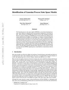
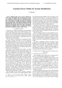
(a) Dependence among input and output in a chain

(b) Dependence of latent functions

Figure 1: Directed graph for a sequence labeling problem The PL model is different from a locally normalized model like maximum entropy markov model (MEMM) as each output component depends on several other output components. Therefore, PL models do not suffer from the label bias problem (Noah, 2011) unlike MEMM. However, PL models create cyclic dependencies among the output components (Heckerman et al., 2001). Figure 1(a) depicts the cyclic dependencies arising in a sequence labeling problem, when the label of an output component is assumed to depend on the labels of the neighboring output components. The presence of cycles makes inference hard for PL models. In Section 5, we discuss an efficient approach to perform inference in such models. The label of an output component need not depend on the labels of all other output components. The dependencies among these output components are captured through the set S. We assume that all the output components have the same dependency relations with other output components. Such an assumption is only for the sake of clarity in presentation and does not restrict our model to be applied to the situations where each output component is associated with different dependency relations. Consider the

5

directed graph in Figure 1(a) for a sequence labeling problem, where each output component is assumed to depend only on the neighboring output components. Here, the dependency set S = {1, 2}, where 1 denotes the dependence of an output component on the previous output component and 2 denotes its dependence on the next output component. One can also consider a model where an output component depends on previous two output components and next two output components. The dotted line in 1(a) shows such a dependency for first and third output component, in which case S = {1, 2, 3, 4}. Let R denote the number of dependency relations in a set S (that is, the cardinality of S) and we assume it to be the same for all the output components. Taking into account those dependencies, we redefine the likelihood in (3) as p(yn |xn ) ∝

L Y

S p(ynl |xnl , ynl ).

(4)

l=1 S d R Here, ynl denotes the labels of a set of output components {ynl }d=1 defined by the S 1 2 } = {yn(l−1) , dependency set S. For the directed graph in Figure 1(a), ynl = {ynl , ynl yn(l+1) }. In (4), instead of conditioning on the rest of the labels, we condition ynl only on the labels defined by the dependency set S. This greatly reduces the computational overhead as we need to consider only those dependencies defined by S. The likelihood (4) is amenable to model data sets with missing labels. If labels of some of the output components are missing, the likelihood (4) can be computed by just ignoring those components and the dependencies using the labels of those components. S The likelihood p(ynl |xnl , ynl ) is defined using a set of latent functions. We use different latent functions to model different dependencies. The dependency of the label ynl on xnl is defined as a local dependency and is modeled as in GP multi-class classification. We associate a latent function with each label in the set {1, 2, . . . Q}. The latent function associated with a label q, denoted as f U q , is called a local latent function. It is defined over all training input components xnl for every n and l and the latent function values associated with a particular label q over N L training examples are denoted by f Uq . The local latent functions associated with a particular input comUQ U U1 ponent xnl are denoted as fnl = {fnl , . . . , fnl }. We also associate a latent function Sd f with each dependency relation d ∈ S and call them as dependent latent functions. These latent functions are defined over all the values of a pair of labels (ˆ ynl , ynl ) where yˆnl ∈ {1, 2, . . . Q} and ynl ∈ {1, 2, . . . Q}. The latent function values associated with a particular dependency d over Q2 label pair values are denoted by f Sd . The dependence of various latent functions on the input and output components for the directed graph in Figure 1(a) is depicted in Figure 1(b). Given these latent functions we define S the likelihood p(ynl |xnl , ynl ) to be a member of an exponential family. S Sd R }d=1 ) = p(ynl |xnl , ynl , {f Uq }Q q=1 , {f P R d U ynl , ynl )) exp(f (xnl ) + d=1 f Sd (ynl P PQ R d , y )) U y Sd nl (xnl ) + d=1 f (ynl nl ynl =1 exp(f

(5)

This differs from the softmax likelihood (2) used in multi-class classification in that it captures the dependencies among output components. Given the latent functions and 6

N the input X = {xn }N n=1 , the likelihood of the output Y = {yn }n=1 is Sd R p(Y|X, {f Uq }Q }d=1 ) = q=1 , {f N Y L Y

Sd R p(ynl |xnl , yn {Dnl } , {f Uq }Q }d=1 ). q=1 , {f

(6)

n=1 l=1 Sd R }d=1 . We define independent GP priors over the latent functions {f U q }Q q=1 , {f Uq The latent function f is given a zero mean GP prior with covariance function K U q . Thus, f Uq is a Gaussian with mean 0 and covariance KUq of size N L × N L, that is p(f Uq ) = N (f Uq ; 0, KUq ). KUq consists of covariance function evaluations over N all pairs of training data input components {{xnl }L l=1 }n=1 . Let θq be the hyperUq parameters associated with K . The latent function f Sd is given zero mean GP prior with an identity covariance which is defined to be 1 when inputs are same and 0 otherwise. Thus f Sd is a Gaussian with mean 0 and covariance I of size Q2 , that is p(f Sd ) = N (f Sd ; 0, IQ2 ). Let f U = (f U1 , f U2 , . . . , f UQ ) be the collection of all local latent functions and f S = (f S1 , f S2 , . . . , f SR ) be the collection of all dependent latent functions. Then the prior over f U and f S is defined as  U   U  f K 0 U S p(f , f |X) = N ; 0, , (7) fS 0 KS

where KU = diag(KU1 , KU2 , . . . , KUQ ) is a block diagonal matrix and KS = IQ2 ⊗ IP . The posterior over the latent functions p(f U , f S |D) is p(f U , f S |X, Y) =

1 p(Y|X, f U , f S )p(f U , f S |X) p(Y|X)

(8)

R where p(Y|X) = p(Y|X, f U , f S )p(f U , f S |X)df U df S is called the evidence. Evidence is a function of hyper-parameters θ = (θ1 , θ2 , . . . , θQ ) and is maximized to estimate them. For notational simplicity, we suppress the dependence of evidence, posterior and prior on the hyper-parameter θ. Due to the non-Gaussian nature of the likelihood, evidence is intractable and the posterior cannot be determined exactly. We use variational inference technique to obtain an approximate posterior. Variational inference is faster than sampling based techniques used in Bratieres et al. (2014a) and does not suffer from convergence problems (Murphy, 2012). It can easily handle multiclass problems and is scalable to models with a large number of parameters. Further, it provides an approximation to the evidence which is useful in estimating the hyperparameters of the model.

4

Variational Inference

Variational Inference technique (Murphy, 2012) approximates the intractable posterior by a tractable approximate distribution. It approximates the posterior p(f |X, Y) by a variational distribution t(f |γ), where f = (f U , f S ) and γ represents the variational 7

parameters. In variational inference, this is done by minimizing the Kullback-Leibler (KL) divergence between t(f |γ) and p(f |X, Y). This can be written as KL(t(f |γ)||p(f |X, Y)) = −L(θ, γ) + log p(Y|X) Z where L(θ, γ) = −KL(t(f |γ)||p(f |X)) + t(f |γ) log p(Y|X, f )df

(9) (10)

Since log p(Y|X) is a constant independent of variational parameters γ, we can estimate γ by maximizing the quantity L(θ, γ). Since KL divergence is always nonnegative, L(θ, γ) acts as a lower bound to the logarithm of evidence. The lower bound L(θ, γ) can also be obtained from the logarithm of evidence by introducing variational distribution and applying Jensen’s inequality. When approximate distribution is same as the posterior (in which case the KL divergence in (9) is zero), the lower bound L(θ, γ) becomes equal to the logarithm of evidence. Hence, we can estimate the hyper-parameters γ and variational parameters θ by maximizing the lower bound L(θ, γ). We use a variational Gaussian (VG) approximate inference approach (Opper and Archambeau, 2009) where the variational distribution is assumed to be a Gaussian. Variational Gaussian approaches can be slow because of the requirement to estimate the covariance matrix. Fortunately, recent advances in VG inference approaches (Opper and Archambeau, 2009) enable one to compute the covariance matrix using O(N L) variational parameters. In fact, we use the VG approach for GPs (Khan et al., 2012) which requires computation of only O(N L) variational parameters, but at the same time uses a concave variational lower bound. We assume the variational distribution t(f |γ) takes the form of a Normal distribution and factorizes as t(f U |γ U )t(f S |γ U ) where γ = {γ U , γ S }. Let t(f U |γ U ) = N (f U ; mU , VU ) where γ U = {mU , VU } and t(f S ) = N (f S ; mS , VS ) where γ S = {mS , VS }. Then, the variational lower bound L(θ, γ) can be written as 1 (log |VU ΩU | + log |VS ΩS | − tr(VU ΩU ) − tr(VS ΩS ) − 2 L N X X > > Et(f U |γ U )t(f S |γ S ) [log p(ynl |xnl , yn {S} , f )](11) mU ΩU mU − mS ΩS mS ) + L(θ, γ) =

n=1 l=1

R −1 −1 where ΩU = KU , ΩS = KS and Et(x) [f (x)] = f (x)t(x)dx represents the expectation of f (x) with respect to the density t(x). Since KU is block diagonal, its inverse is block diagonal, and hence ΩU is block diagonal that is ΩU = −1 diag(ΩU1 , ΩU2 , . . . , ΩUQ ), where ΩUq = KUq . Similarly, ΩS is also block diagonal with each block being a diagonal matrix IQ2 . The marginal variational distribution of local latent function values f Uq is a Gaussian with mean mUq and covariance VUq , and that of dependent latent function values f Sd is a Gaussian with mean mSd and covariance VSd . The variational lower bound L(θ, γ) requires computing an expectation of the log likelihood with respect to the variational distribution. However, the integral is intractable since the likelihood is a softmax function. So, we use Jensen’s inequality to obtain a tractable lower bound to the expectation of log likelihood. The variational lower bound L(θ, γ) can be written as 8

L(θ, γ) =

Q > 1 X (log |VUq ΩUq | − tr(VUq ΩUq ) − mUq ΩUq mUq ) 2 q=1

+

R X
> (log |VSd ΩSd | − tr(VSd ΩSd ) − mSd ΩSd mSd ) d=1

+

N X L  X n=1 l=1

Uy

mnl nl +

R X

mSd (y d

nl

,ynl ) − log

Q X

q exp(mU nl

q=1

d=1

R X
 1 Sd 1 Uq + V(yd ,q),(yd ,q) ) mSd + V(nl,nl) d ,q) + (ynl nl nl 2 2

(12)

d=1

Uq Q Sd R The variational parameters γ = {{mUq }Q }q=1 , {mSd }R }d=1 } q=1 , {V d=1 , {V are estimated by maximizing the variational lower bound (12). Note that the variational parameters VUq and VSd represent covariance matrices and hence the maximization is done under the constraint that they are positive semi-definite (p.s.d.). The lower bound (12) does not contain any cross-covariance term across the labels and hence, the covariance matrix VU is block diagonal that is VU = diag(VU1 , . . . , VUQ ). Similarly, VS is also block diagonal that is VS = diag(VS1 , . . . , VSR ). The lower bound is jointly concave with respect to all the variational parameters. This can be verified by noting that ΩUq and ΩSd are p.s.d. (inverse of a covariance matrix), log determinant is a concave function, trace of a p.s.d. matrix is a convex function and log sum exponential is a convex function (Boyd and Vandenberghe, 2004). The variational parameters are estimated using a co-ordinate ascent approach. We repeatedly estimate each variational parameter while keeping the others fixed. The variational mean parameters mUq and mSd are estimated using gradient based approaches. The variational covariance matrices VUq and VSd are estimated under the p.s.d. constraint. This can be done efficiently using the fixed point approach mentioned in Khan et al. (2012). It is reported to converge faster than other VG approaches for GPs and is based on a concave objective function similar to (12). The approach maintains the p.s.d. constraint on the covariance matrix and computes VUq by estimating only O(N L) variational parameters. The requirement of only O(N L) variational parameters to compute VUq can be seen by considering the gradient of (12) with respect to VUq . Equating the gradient to zero, at the point of maximum we can see that VUq takes the form VUq = (ΩUq + diag(λ))−1 , where λ is a vector of size N L which we have to estimate. Estimation of VUq using the fixed point approach converges since (12) is strictly concave with respect to VUq . We note that the variational covariance matrix VSd is diagonal since ΩSd is diagonal. Hence, for computing a p.s.d. VSd we need to estimate only the diagonal elements of VSd under the element-wise non-negativity constraint. This can be done easily using gradient based methods. The variational parameters γ are estimated for a particular set of hyper-parameters θ. The hyper-parameters θ are also estimated by maximizing the lower bound (12). The variational parameters γ and the model parameters θ are estimated alternately following a variational expectation maximization (EM) approach. This results in a faster convergence (Murphy, 2012). In the E-step, the variational distribution is computed

9

Algorithm 1 Model selection and inference in Gaussian process sequence labeling model 1: Input: Training data (X, Y), dependency set S 2: Initialize hyper-parameters θ, variational parameters γ 3: repeat 4: repeat 5: for q = 1 to Q do 6: Update mUq by maximizing (12) w.r.t mUq 7: Update VUq by maximizing (12) w.r.t VUq 8: end for 9: for d = 1 to R do 10: Update mSd by maximizing (12) w.r.t mSd 11: Update VSd by maximizing (12) w.r.t VSd 12: end for 13: until relative increase in lower bound (12) is small 14: Update θ by maximizing (12) w.r.t θ 15: until relative increase in lower bound (12) is small 16: Return: θ, γ

by maximizing the lower bound with respect to the variational parameters γ. In the M-step, the lower bound is maximized with respect to the hyper-parameters θ. This step can be seen as a maximum marginal likelihood estimation of the hyper-parameters using expected log likelihood, where the expectation is taken with respect to the variational distribution computed in the E-step. In the ideal case when the KL divergence between the variational distribution and the posterior distribution vanishes the lower bound becomes the same as the logarithm of evidence. Algorithm 1 summarizes various steps involved in our approach. The variational lower bound (12) is strictly concave with respect to each of the variational parameters. Hence, the estimation of variational parameters using co-ordinate ascent algorithm (inner loop) converges (Bertsekas, 1999). Convergence of EM for exponential family guarantees the convergence of Algorithm 1. The overall computational complexity of Algorithm 1 is dominated by the computation of VUq . It takes O(QN 3 L3 ) time as it requires inversion of Q covariance matrices of size N L × N L. The computational complexity for estimating VSd is O(RN LQ) and is negligible compared to the estimation of VUq . Note that the computational complexity of the algorithm increases linearly with respect to the number of dependencies R. Algorithm 1 can be easily parallelized to improve the performance. By parallelizing the estimation of the variational parameters (inner loop), one can obtain considerable speed- up in running time when the number of labels Q or the number of dependencies R is large.

5

Prediction

The variational posterior distributions estimated using VG approximation t(f U ) = QQ QQ QR QR Uq Uq Sd ) = ; mUq , VUq ) and t(f S ) = ) = q=1 t(f q=1 N (f d=1 t(f d=1 10

N (mSd , VSd ) can be used to predict the structured test output y∗ for a test input x∗ . The predictive probability of labeling a component of the output y∗l given x∗l and rest of the labels y∗ \y∗l is Z p(y∗l |x∗l , y∗ \y∗l ) = p(y∗l |x∗l , y∗ \y∗l , f∗ )p(f∗ )df∗ PR Z U y∗l d exp(f∗l + d=1 f∗Sd (y∗l , y∗l )) = PR PQ U y∗l d , y )) Sd + d=1 f∗ (ynl nl y∗l =1 exp(f∗l Uq Q Uq Q Sd R {p(f∗l )}q=1 {p(f∗Sd )}R d=1 {d(f∗l )}q=1 {d(f∗ )}d=1

(13)

where p(f∗ ) denotes the predictive distribution of all latent function values for the test Uq input x∗ . In (13), p(f∗l ) represents the predictive distribution of local latent function q Uq q for a test input component x∗l . This is Gaussian with mean mU ∗l and variance v∗l where, >

q Uq mU ΩUq mUq ∗l = K∗l Uq v∗l

=

Uq K∗l,∗l

−

and

> KUq (ΩUq ∗l

− ΩUq VUq ΩUq )KUq ∗l .

Here, KUq ∗l is an N L dimensional vector obtained from the kernel evaluations for the Uq label q between test input data component x∗l and training data X and K∗l,∗l represents Sd the kernel evaluation of the test data input component x∗l with itself. f is independent of test data input and the predictive distribution p(f∗Sd ) is the same as p(f Sd ). This is a Gaussian with mean mSd and covariance VSd . The computation of the expected value of softmax with respect to the latent functions (13) is intractable. Instead we compute softmax of the expected value of the latent functions and use a normalized probabilistic score. PR y∗l U y∗l 1 Dd + d=1 mDd exp(mU + 21 v∗l d ,y ) + 2 V(y d ,y ),(y d ,y ) ) ∗l (y∗l ∗l ∗l ∗l ∗l ∗l N S(y∗l , x∗l ) = PQ P R Uq 1 Uq 1 Dd Dd v V exp(m + + m + q=1 d=1 ∗l 2 ∗l 2 (y d ,q),(y d ,q) ) (y d ,q) ∗l

∗l

∗l

The maximum of the normalized score can be used to decide the label y∗l for the input x∗l . In practice, while predicting the label for x∗l , the true labels associated with the dependencies S will not be available. In fact, the labels associated with the dependencies also need to be predicted. Under such noisy circumstances, relying on a single label (one with maximum probability) associated with a dependency will not yield good results in general. We refine the normalized score (RN S) to take into account this uncertainty. PR U y∗l y∗l Dd Dd + d=1 Ey∗l + 12 V(y ]) exp(mU + 12 v∗l d [m d d d ∗l (y∗l ,y∗l ) ∗l ,y∗l ),(y∗l ,y∗l ) RN S(y∗l , x∗l ) = PQ P R Uq 1 Uq Dd Dd + 12 V(y d [m d d ,q),(y d ,q) ]) q=1 exp(m∗l + 2 v∗l + d=1 Ey∗l (y ,q) ∗l

∗l

∗l

Here, we use the expected value over all possible labelings associated with a dependency d. The expectation is computed P using the RN S value associated with the labels Q d d y∗l for the input xd∗l , that is, Ey∗l RN S(y∗l , xd∗l )[·]. d [·] = y d =1 ∗l

11

Algorithm 2 Prediction in Gaussian process sequence labeling model Sd R }d=1 Input: Test data x∗ = (x∗1 , . . . , x∗L ), posterior mean {mUq }Q q=1 and {m Sd R Uq Q and posterior covariance {V }q=1 and {V }d=1 Uq Q Uq Q L 2: Obtain predictive means {{m∗l }q=1 }L l=1 , and variances {{v∗l }q=1 }l=1

1:

Uy

3:

Initialize : RN S 0 (y∗l , x∗l ) =

Uy

exp(m∗l ∗l + 21 v∗l ∗l ) PQ Uq 1 Uq q=1 exp(m∗l + 2 v∗l )

∀ y∗l = 1, . . . , Q, ∀ l =

1...,L Initialize : t = 0 repeat 6: t=t+1 7: for l = 1 to L do 8: for y∗l = 1 to Q do 4: 5:

9:

t

RN S (y∗l , x∗l ) =

P Uy Uy Dd Dd 1 exp(m∗l ∗l + 12 v∗l ∗l + R d=1 Ey d [m(y d ,y ) + 2 V(y d ,y ),(y d ,y ) ]) ∗l ∗l ∗l ∗l ∗l ∗l ∗l PR PQ Uq 1 Uq 1 Dd ]) + 2 VDdd q=1 exp(m∗l + 2 v∗l + d=1 Ey d [m d d (y

10: 11: 12: 13: 14: 15:

,q)

(y

,q),(y

,q)

∗l ∗l ∗l ∗l PQ t−1 d d where Ey∗l RN S (y , x )[·] d [·] = d =1 ∗l ∗l y∗l end for end for until change in RN S t w.r.t RN S t−1 is small (ˆ y∗1 , . . . , yˆ∗L ) = (argmaxy∗1 RN S t (y∗1 , x∗1 ), . . . , argmaxy∗L RN S t (y∗L , x∗L )) Return: (ˆ y∗1 , . . . , yˆ∗L )

We provide an iterative approach to estimate the labels of the test output y∗ = (y∗1 , . . . , y∗L ) for the test input x∗ = (x∗1 , . . . , x∗L ). We compute the RN S value for all possible labelings of the pair {(y∗l , x∗l )}N l=1 . An initial RN S value is computed without considering the dependencies. We iteratively refine the RN S value using the previously computed RN S value by taking into account the dependencies. The process is continued until convergence, that is when no change is observed on successive RN S values. The final RN S value is used to make predictions for the test input. Prediction is done separately for each y∗l by assigning labels with maximum RN S value for x∗l . The computational complexity of Algorithm 2 is O(Q2 RL). The algorithm converges after a few iterations. The convergence condition for a fixed point algorithm similar to Algorithm 2 is discussed in Li et al. (2013). In our experiments, we found that the algorithm converges in 5 iterations on an average.

6

Experimental Results

We conduct experiments to study the generalization performance of the proposed Gaussian Process Sequence labeling (GPSL) model. We use the sequence labeling problems in natural language processing to study the behavior of the proposed approach. Although, the proposed approach is general and can handle dependencies of any length, we consider three different models of the proposed approach in our experiments. The first model, GPSL1, assumes that the current label depends only on the previous label. The second model, GPSL2, assumes that the current label depends both on the previous 12

Table 1: Properties of the sequence labeling datasets

number of labels number of features training data size/ test data size

Base NP 3 6438

Chunking 14 29764

Segmentation 2 1386

150/150

50/50

20/16

and the next label in the sequence. The third model, GPSL4, assumes that the current label depends on the previous and the next two labels. We consider three sequence labeling problems in natural language processing to study the performance of the proposed approach. The dataset for all these problems are obtained from the CRF++1 toolbox. We provide a brief description of the three sequence labeling problems. Noun phrase identification Noun phrases in a sentence have noun as its head. The starting word in the noun phrase is given a label B, while the words inside the noun phrase are given a label I. All the other words are given a label O. The task here is to assign each word with a label from the set {B, I, O}. We use the BaseN P dataset to perform the task. From the BaseN P dataset, we randomly choose 150 sentences for training and test the performance on 150 sentences. Chunking Shallow parsing or chunking identifies constituents in a sentence such as noun phrase, verb phrase etc. Here, each word in a sentence is labeled as belonging to verb phrase, noun phrase etc. In the Chunking dataset, words are assigned a label from a set of size 14. In this task, we consider 50 sentences for training and 50 sentences for testing, all randomly chosen from the Chunking dataset. Segmentation Segmentation is the process of finding meaningful segments in a text such as words, sentences etc. We consider a word segmentation problem where the words are identified from a Chinese sentence. The Segmentation data set assigns each unit in the sentence a label denoting whether it is beginning of a word (B) or inside a word (I). The task is to assign either of these two labels to each unit in a sentence. We consider 20 training set sentences and 16 test set sentences randomly chosen from the Segmentation dataset for the task. In all these data sets except Segmentation, a sentence is considered as an input and words in the sentence as input components. In Segmentation, every alphabet is considered as an input component. The features for each input component are extracted using the template files provided in the CRF++ package. The properties of all the data sets are summarized in the Table 1. 1 Available

at http://crfpp.googlecode.com/svn/trunk/doc/index.html

13

Table 2: Comparison of the performance of GPSL1, GPSL2, GPSL4, SSVM, CRF and GPstruct on three sequence labeling problems using average Hamming loss (in percentage). The numbers in bold face style indicate the best results among these approaches.

GPSL1 GPSL2 GPSL4 CRF SSVM GPstruct

Base NP 5.75±0.98 5.55±0.92 5.54±0.94 5.21±0.84 5.19±0.91 5.66±0.93

Chunking 13.61±1.87 12.69±1.69 12.70±1.79 11.76±1.73 10.71±1.49 12.56±1.82

Segmentation 24.25±2.95 23.62±2.85 23.60±2.81 24.10±3.49 23.46±3.45 23.79±2.90

We compare the performance of the proposed approach with popular sequence labeling approaches, structural SVM (SSVM) (Balamurugan et al., 2011)2 , conditional random field (CRF) (Bottou, 2010)3 , and GPstruct (Bratieres et al., 2014a)4 . All the models used a linear kernel. GPstruct experiments are run for 100000 elliptical slice sampling steps. The performance is measured in terms of average Hamming loss over all test data points. The Hamming loss between PL the actual test output y∗ and predicted test output y ˆ∗ is given by Loss(y∗ , y ˆ∗ ) = l=1 I(y∗l 6= yˆ∗l ), where I(·) is the indicator function. Table 2 compares the performance (percentage of the average Hamming loss) of various approaches on the three sequence labeling problems. The GPSL models, SSVM, CRF and GPstruct are run over 10 independent partitions of the data set5 and a mean of the Hamming loss over all partitions along with the standard deviation are reported in Table 2. The reported results suggest that the GPSP models with higher dependencies performed better than GPstruct on BaseN P and Segmentation. The performance of GPSP models are close to CRF in these data sets as we increase the number of dependencies but not as good as SSVM. However, GPSP models have the advantage of being Bayesian and can provide confidence over predictions. The GPSL model which considered only the previous label did not demonstrate a good performance while the one which considered both the previous and next label (GPSL2) gave a much better performance. The performance of the GPSL model which considered the previous and the next 2 labels (GPSL4) improved only marginally compared to GPSL2 on these data sets. We note that increasing the number of dependencies beyond four did not bring any improvement in performance for the sequence labeling data sets that we have considered. The proposed GPSL approach is implemented in Matlab. The GPSL Matlab programs are run on a 3.2 GHz Intel processor with 4GB of shared main memory under Linux. The SSVM approach is implemented in C, the CRF approach is coded in C++ and the GPStruct approach is in python. Since the implementation languages differ, it is unfair to make a runtime comparison of various approaches. Table 3 compares the 2 Code

available at http://drona.csa.iisc.ernet.in/∼shirish/structsvm sdm.html available at http://leon.bottou.org/projects/sgd#stochastic gradient descent version 2 4 Code available at https://github.com/sebastien-bratieres/pygpstruct 5 The train and test set partitions are different from those used by Bratieres et al. (2014a).

3 Code

14

Table 3: Comparison of running time (in seconds) of the various GPSP models and GPstruct Data GPSL1 Segmentation 17.13 Chunking 1.09e+03 Base NP 6.01e+03

GPSL2 GPSL4 GPstruct 19.64 22.83 3.82e+03 1.35e+03 1.71e+03 4.56e+04 6.69e+03 7.25e+03 7.54e+04

average runtime (in seconds) of the various GPSL models and GPstruct on the sequence labeling data sets. We find that the GPSL models are an order of magnitude faster than GPStruct. We also find that using more dependencies resulted in only a slight increase in runtime.

6.1

Experiments with Missing Labels

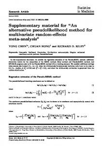
In many sequence labeling tasks such as sequence labeling problems arising in natural language processing, the labels of some of the output components might be missing in the training data set. This arises when the experts labeling an example are unsure of the label to be assigned to a particular component of the example. This is common when crowd sourcing techniques are employed to obtain the labels. GPSL models are useful to learn from the data sets with missing labels due to its ability to capture larger dependencies. We study the ability of the proposed GPSL models to handle sequence labeling data sets with missing labels. We learn the GPSL models from the sequence labeling data sets with some fraction of the labels missing. We vary the fraction of missing labels and study how the performance of our model varies with respect to missing labels. Figure 2 provides the variation in performance of various GPSL models as we vary the fraction of missing labels from the sequence labeling data sets such as BaseN P , Chunking, and Segmentation. The performance is measured in terms of accuracy which is obtained by subtracting the average Hamming loss from 1. The experiments are repeated 5 times and the mean accuracy is plotted in Figure 2. We find that the performance of the GPSL models does not significantly degrade as the fraction of the missing labels increases. Figure 2 shows that GPSL4 which uses the previous and the next 2 labels provides a better performance than other GPSL models. GPSL4 learns a better model by considering a larger neighborhood information. When some labels are missing, by making use of a larger neighborhood, GPSL4 can capture some dependencies which enable it to learn a better model. Thus, the GPSL models which consider more dependencies are extremely useful to handle data sets with missing labels.

7

Conclusion

We proposed a novel Gaussian Process approach to perform sequence labeling based on pseudo-likelihood approximation. The use of pseudo-likelihood enabled the model to capture long range dependencies without becoming computationally intractable. The approach can be readily applied to data sets with missing labels. The approach used a

15

faster inference scheme based on variational inference. We also proposed an approach to perform prediction which makes use of the information from the neighboring labels. The proposed approach is useful for a wide range of sequence labeling problems arising in natural language processing. Experimental results showed the effectiveness of the proposed approach in sequence labeling problems. The ability of the proposed approach to capture long range dependencies was found to be extremely useful in handling data sets with missing labels. Acknowledgements We thank M. E. Khan for kindly providing the matlab code of the variational Gaussian approach (Khan et al., 2012) for the binary classification problem.

References Y. Altun, T. Hofmann, and A. J. Smola. Gaussian Process Classification for Segmenting and Annotating Sequences. In ICML, 2004. P. Balamurugan, S. Shevade, S. Sundararajan, and S.S. Keerthi. A Sequential Dual Method for Structural SVMs. In SDM, pages 223–234, 2011. D. P. Bertsekas. Nonlinear Programming. Athena Scientific, 1999. J. Besag. Statistical analysis of non-lattice data. The Statistician, 24:179–195, 1975. L. Bottou. Large-Scale Machine Learning with Stochastic Gradient Descent. In COMPSTAT, 2010. S. Boyd and L. Vandenberghe. Convex Optimization. Cambridge University Press, 2004. S. Bratieres, N. Quadrianto, and Z. Ghahramani. Bayesian Structured Prediction Using Gaussian Processes. IEEE transactions on Pattern Analysis and Machine Intelligence, 2014a. S. Bratieres, N. Quadrianto, S. Nowozin, and Z. Ghahramani. Scalable Gaussian Process Structured Prediction for Grid Factor Graph Applications. ICML, 2014b. K. M. A. Chai. Variational Multinomial Logit Gaussian Process. J. Mach. Learn. Res., 13, 2012. M. Girolami and S. Rogers. Variational Bayesian Multinomial Probit Regression with Gaussian Process Priors. Neural Computation, 18(8):1790–1817, 2006. D. Heckerman, D. M. Chickering, C. Meek, R. Rounthwaite, and C. Kadie. Dependency Networks for Inference, Collaborative Filtering, and Data Visualization. J. Mach. Learn. Res., 1:49–75, 2001. M. E. Khan, S. Mohamed, and K. P. Murphy. Fast Bayesian Inference for NonConjugate Gaussian Process Regression. In NIPS, pages 3149–3157, 2012. 16

J. D. Lafferty, A. McCallum, and F. C. N. Pereira. Conditional Random Fields: Probabilistic Models for Segmenting and Labeling Sequence Data. In ICML, pages 282– 289, 2001. J. D. Lafferty, X. Zhu, and Y Liu. Kernel Conditional Random Fields: Representation and Clique Selection. In ICML, volume 69, 2004. Q Li, J Wang, D. P. Wipf, and Z. Tu. Fixed-Point Model For Structured Labeling. In ICML, pages 214–221, 2013. K. P. Murphy. Machine learning: A Probabilistic Perspective. The MIT Press, 2012. A. S. Noah. Linguistic Structure Prediction . Morgan and Claypool, 2011. M. Opper and C. Archambeau. The Variational Gaussian Approximation Revisited. Neural Computation, 21:786–792, 2009. Y. Qi, M. Szummer, and T. P. Minka. Bayesian conditional random fields. Proc. AISTATS 2005, 2005. C. E. Rasmussen and C. K. I. Williams. Gaussian Processes for Machine Learning (Adaptive Computation and Machine Learning). MIT Press, 2005. C. Sutton and A. McCallum. Piecewise Pseudolikelihood for Efficient Training of Conditional Random Fields. ICML, pages 863–870, 2007. K. Toutanova, D. Klein, C. D. Manning, and Y. Singer. Feature-Rich Part-of-Speech Tagging with a Cyclic Dependency Network. In HLT-NAACL, pages 252–259, 2003. I. Tsochantaridis, T. Joachims, T. Hofmann, and Y. Altun. Large Margin Methods for Structured and Interdependent Output Variables. J. Mach. Learn. Res., 6:1453–1484, 2005. C. K. I. Williams and D. Barber. Bayesian Classification With Gaussian Processes. IEEE Transactions on Pattern Analysis and Machine Intelligence, 20(12):1342– 1351, 1998.

17

(a) Chunking

(b) Base NP

(c) Segmentation

Figure 2: Variation in accuracy as the fraction of missing labels is varied from 0.05 to 0.5

18