Gaussian Process Regression for Sensor ... - Semantic Scholar

IEEE TRANSACTIONS ON SIGNAL PROCESSING, VOL. 61, NO. 2, JANUARY 15, 2013

223

Gaussian Process Regression for Sensor Networks Under Localization Uncertainty Mahdi Jadaliha, Yunfei Xu, Jongeun Choi, Nicholas S. Johnson, and Weiming Li

Abstract—In this paper, we formulate Gaussian process regression with observations under the localization uncertainty due to the resource-constrained sensor networks. In our formulation, effects of observations, measurement noise, localization uncertainty, and prior distributions are all correctly incorporated in the posterior predictive statistics. The analytically intractable posterior predictive statistics are proposed to be approximated by two techniques, viz., Monte Carlo sampling and Laplace’s method. Such approximation techniques have been carefully tailored to our problems and their approximation error and complexity are analyzed. Simulation study demonstrates that the proposed approaches perform much better than approaches without considering the localization uncertainty properly. Finally, we have applied the proposed approaches on the experimentally collected real data from a dye concentration field over a section of a river and a temperature field of an outdoor swimming pool to provide proof of concept tests and evaluate the proposed schemes in real situations. In both simulation and experimental results, the proposed methods outperform the quick-and-dirty solutions often used in practice. Index Terms— Gaussian processes, Monte Carlo methods, regression analysis, sensor networks, Laplace’s methods.

I. INTRODUCTION

R

ECENTLY, there has been a growing interest in wireless sensor networks due to advanced embedded network technology. Their applications include, but are not limited to, environment monitoring, building comfort control, traffic control, manufacturing and plant automation, and surveillance

Manuscript received April 20, 2012; accepted September 28, 2012. Date of publication October 09, 2012; date of current version December 20, 2012. The associate editor coordinating the review of this manuscript and approving it for publication was Dr. Z. Jane Wang. This work has been supported, in part, by the National Science Foundation through CAREER Award CMMI-0846547. This article is Contribution 1713 of the U.S. Geological Survey Great Lakes Science Center. In-stream field experiments were supported by the Great Lakes Fishery Commission. The work of W. Li was supported in part by the National Science Foundations Awards IOB0517491 and IOB0450916. This support is gratefully acknowledged. Use of trademark names does not represent endorsement by the U.S. Government. M. Jadaliha and Y. Xu are with the Department of Mechanical Engineering, Michigan State University, MI 48824 USA (e-mail: [email protected]; [email protected]). J. Choi is with the Departments of Mechanical Engineering and Electrical and Computer Engineering, Michigan State University, MI 48824 USA (e-mail: [email protected]). N. S. Johnson is with United States Geological Survey, Great Lakes Science Center, Hammond Bay Biological Station, Millersburg, MI 49759 USA (e-mail: [email protected]). W. Li is with the Department of Fisheries and Wildlife, Michigan State University, East Lansing, MI 48824 USA (e-mail: [email protected]). Color versions of one or more of the figures in this paper are available online at http://ieeexplore.ieee.org. Digital Object Identifier 10.1109/TSP.2012.2223695

systems [1], [2]. Mobility in a sensor network can increase its sensing coverage both in space and time, and robustness against uncertainties in environments. Exploitation of mobile sensor networks has been increased in collecting spatio-temporal data from the environment [3]–[5]. Gaussian process regression (or Kriging in geostatistics) has been widely used to draw statistical inference from geostatistical and environmental data [6], [7]. Gaussian process modeling enables us to predict physical values, such as temperature or harmful algae bloom biomass, at any point and time with a predicted uncertainty level. For example, near-optimal static sensor placements with a mutual information criterion in Gaussian processes were proposed in [8], [9]. A distributed Kriged Kalman filter for spatial estimation based on mobile sensor networks was developed in [5]. Centralized and distributed navigation strategies for mobile sensor networks to move in order to reduce prediction error variances at points of interest were developed in [10]. Localization in sensor networks is a fundamental problem in various applications to correctly fuse the spatially collected data and estimate the process of interest. However, obtaining precise localization of robotic networks under limited resources is very challenging [11], [12]. Among the localization schemes, the range-based approach [13], [14] provides higher precision as compared to the range-free approach that could be cost-effective. The global positioning system (GPS) becomes one of the major absolute positioning systems in robotics and mobile sensor networks. Most of affordable GPSs slowly update their measurements and have resolution worse than one meter. A GPS is often augmented by the inertial navigation system (INS) for better resolution [15]. In practice, resource-constrained sensor network systems are prone to large uncertainty in localization. Most previous works on Gaussian process regression for mobile sensor networks [6], [9], [10], [16] have assumed that the exact sampling positions are available, which is not practical in real situations. Therefore, motivated by the aforementioned issues, we consider correct (Bayesian) integration of uncertainties in sampling positions, and measurements noise for Gaussian process regression and its computation error and complexity analysis for the sensor network applications. The overall picture of our work is similar to the one in [17] in which an extended Kalman filter (EKF) was used to incorporate robot localization uncertainty and field parameter uncertainty. However, [17] relies on a parametric model, which is a radial basis function network model and EKF, while our motivation is to use more flexible non-parametric approach, viz., Gaussian process regression taking into account localization uncertainty in a Bayesian framework.

1053-587X/$31.00 © 2012 IEEE

224


Fig. 1. The prediction results of applying Gaussian process regression on the true and noisy sampling position are shown. The first, second, and third rows correspond to the prediction, prediction error variance, and squared empirical error (between predicted and true fields) fields. The first column shows the result of applying Gaussian process regression on the true sampling positions. Second and third columns show the results of applying Gaussian process regression on the and noise covariance matrices, respectively. True and noisy sampling positions are shown in circles with noisy sampling positions with agent indices in the second row.

Gaussian process regression in [18] integrate uncertainty in the test input position for multiple-step ahead time series forecasting. In [18], uncertainty was not considered in the sampling positions of the training data (or observations). However, localization uncertainty effect is potentially significant. For example, Fig. 1 shows the effect of noisy sampling positions on the results of Gaussian process regression. Note that adding noise to the sampling positions considerably increase the empirical RMS error, shown in the third row of Fig. 1. A Gaussian approximation to the intractable posterior predictive statistics obtained in [18] has been utilized for the predictive control with Gaussian models [19], [20] and Gaussian process dynamic programming [21]. In general, the length of the training data is much longer than that of the test point for sensor network applications, therefore, our problem possibly involves a high dimensional uncertainty vector for the sampling positions. Gaussian process prediction with localization uncertainty can be obtained as a posterior predictive distribution using Bayes’ rule. The main difficulty to this is that it has no analytic closedform solution and has to be approximated either through Monte Carlo sampling [22] or other approximation techniques such as variational inference [23]. As an important analytical approximation technique, Laplace’s method has been known to be useful in many such situations [24], [25]. Different Laplace approximation techniques have been analyzed in terms of approximation error and computation complexity [24]–[27]. The contribution of this paper is as follows. First, we formulate Gaussian process regression with observations under the localization uncertainty due to the resource-constrained

(possibly mobile) sensor networks. Next, approximations have been obtained for analytically intractable predictive mean, and predictive variance by using the Monte Carlo sampling and Laplace’s method. Such approximation methods have been carefully tailored to our problems. In particular, a modified version of the moment generating function (MGF) approximation [25] has been developed as a part of Laplace’s method to reduce the computational complexity. In addition, we have analyzed and compared the approximation error and the complexity so that one can choose a tradeoff between the performance requirements and constrained resources for a particular sensor network application. Another important contribution has been to provide proof of concept tests and evaluate the proposed schemes in real situations. We have applied the proposed approaches on the experimentally collected real data from a dye concentration field over a section of a river and a temperature field of an outdoor swimming pool. The preliminary work of this paper containing only the Laplace methods along with simulation results was reported in [28]. The remainder of this paper is organized as follows. In Section II, we review Gaussian process regression, Monte Carlo sampling and Laplace’s method briefly. In Section III, Gaussian process prediction in the presence of the localization uncertainty has been formulated for a proposed sampling scheme as a Bayesian inference problem. We first present the Monte Carlo estimators for the posterior predictive mean and variance in Section IV. In Section V, using Laplace’s method, we provide approximations for the posterior predictive statistics. Section VI compares the computational cost and

JADALIHA et al.: GAUSSIAN PROCESS REGRESSION FOR SENSOR NETWORKS UNDER LOCALIZATION UNCERTAINTY

225

approximation accuracy over the proposed estimators based on the Mont Carlo sampling and the Laplace’s method. Finally the simulation and experimental results are provided in Sections VII and VIII, respectively. Standard notation will be used throughout the paper. Let , , , , , denote, respectively, the sets of real, non-negative real, positive real, integer, non-negative integer, and positive integer numbers. denotes the identity matrix of size ( for an appropriate dimension.) For column vectors , , and , stacks all vectors to create one column denotes the Euclidean norm (or the vector vector, and 2-norm) of . denotes the determinant of a matrix , and denotes trace of a square matrix . Let and denote, respectively, the expectation and the vari, which ance of a random vector . A random vector is distributed by a multivariate Gaussian distribution of a mean and a variance , is denoted by . We define the first and the second derivative operators on with respect to a vector as follow.

(2)

where . In general, the mean and the covariance functions of a Gaussian process can be estimated a priori by maximizing the likelihood function [16]. Suppose, we have noise corrupted observations without localization error, and . Assume , where is an independent and that identically distributed (i.i.d.) white Gaussian noise with variance . is defined by . The collections of the realizations and the have the Gaussian disobservations tributions

where

is the covariance matrix of obtained by , and is the identity matrix with an of the Gaussian appropriate size. We can predict the value as [7] process at a point

In (2), the predictive mean is (3) .. .

..

.

.. .

and the predictive variance is given by

If there exists and , such that the approximation error satisfies , we say that the error between and is of order and also write . Other notation will be explained in due course.

where obtained by the variance at

(4) is the covariance matrix between and , and is . (3) and (4) can be obtained from the fact that (5)

II. PRELIMINARIES In this section, we review the spatio-temporal Gaussian process, Monte Carlo sampling and Laplace’s method, which will be used throughout the paper. A. Gaussian Process Regression A Gaussian process defines a distribution over a space of functions and it is completely specified by its mean function denote and covariance function. Let contains the sampling lothe index vector, where and the sampling time .A cation Gaussian process, , is formally defined as below. Definition 1: A Gaussian process [7] is a collection of random variables, any finite number of which have a joint Gaussian distribution. For notational simplicity, we consider a zero-mean Gaussian . For example, one may process1 consider a covariance function defined as (1) 1A Gaussian process with a nonzero-mean can be treated by a change of variables. Even without a change of variables, this is not a drastic limitation, since the mean of the posterior process is not confined to zero [7].

Note that the predictive mean in (3) and its prediction error variance in (4) require the inversion of the covariance matrix whose size depends on the number of observations . Hence a drawback of Gaussian process regression is that its computational complexity and memory space increase as more measurements are collected, making the method prohibitive for agents with limited memory and computing power. To overcome this increase in complexity, a number of approximation methods for Gaussian process regression have been proposed. In particular, the sparse greedy approximation method [29], the Nystrom method [30], the informative vector machine [31], the likelihood approximation [32], and the Bayesian committee machine [33] have been shown to be effective for many problems. In particular, it has been proposed that spatio-temporal Gaussian process regression can be applied to truncated observations including only measurements near the target position and time of interest for agents with limited resources [10]. To justify prediction based on only the most recent observations, a similar argument has been made in [34] in the sense that the data from the remote past do not change the predictors significantly under the exponentially decaying correlation functions. In this paper, we also assume that at each iteration the mobile sensor networks only needs to fuse a fixed number of truncated

226


observations, which are near the target points of interest, to limit the computational resources. B. Monte Carlo and Importance Sampling In what follows, we briefly review Monte Carlo and Importance sampling based on [35]. The idea of Monte Carlo simulation is to draw an i.i.d. set of random samples from a target density , where . These random samples will be used to approximate by an empir, where ical point-mass function denotes the Dirac delta. Consequently, the integrals can be approximated with tractable sums that converge as follows.

where is a sequence of i.i.d. random vectors, which is drawn from distribution. In the following theorem, which can be shown to be a special case of the results from [36], we show the convergence properties of the approximation in (7) as functions of , the number of random samples [36]. Theorem 2: (Theorems 1 and 2 from [36]) Consider the given in (7) to the ratio given approximation in (6). If is proportional to a proper probability density function defined on , and , and are finite, we have

where

is an unbiased estimator. In addition, it will almost surely , which can be proved by the asymptotically converge to strong law of large numbers. Considering for simplicity, if satisfies , then the variance of the estimator converges to as increases. In particular, the central limit theorem provides us with convergence in distribution as follows. , where denotes convergence in distribution. Importance sampling is a special case of Monte Carlo implementation, having random samples generated from an available distribution rather than the distribution of interest. Let us introduce an arbitrary importance proposal distribution whose support includes the support of . We can then rewrite as , where is known as the importance weight. Simulating i.i.d. samples according to and evaluating , a possible unbiased Monte Carlo estimate of is given by

.

Under weak assumptions, the strong law of large num. This integration bers applies, yielding method can also be interpreted as a sampling method is approximated by where the posterior density , and

is the integra-

tion of with respect to the empirical measure . In this paper, we shall compute the ratio of two integrals in the form of (6)

Proof: It is a straightforward application of the results from Theorems 1 and 2 in [36] to (6) and (7). C. Laplace Approximations The Laplace method is a family of asymptotic approxima, tions that approximate an integral of a function, i.e., , and . Let the function be in where a form , where , and is a two times continuously differentiable real function on . , i.e., Let denote the exact mode of

Then Laplace’s method produces the approximation [24]: (8)

where . The Laplace approximation in (8) will produce reasonable results as long as the is unimodal or at least dominated by a single mode. . In practice it might be difficult to find the exact mode of A concept of an asymptotic mode is introduced to gauge the approximation error when the exact mode is not used [26]. is called an asymptotic mode of order Definition 3: for if as , and . Suppose that is an asymptotic mode of order for and satisfies the regularity conditions given in Appendix A. Then it follows that we have

, and are defined on a space . To comwhere in (6), we use the following approximation as propute posed in [36].

(9) where

(7)

is given by


More precise form with the asymptotic mode of order is computed for an approximation of order in [27]. In many Bayesian inference applications and as in our problem, we need to compute the ratio of two integrals. To this end, fully exponential Laplace approximations has been developed by [24] to compute Laplace approximations of the ratio of two integrals, i.e.,

method. By using Theorem 5 in [26], the approximation of and its error order are given as

(14)

(10) and has a dominant peak at its maximum, then If each of Laplace’s method may be directly applied to both the numerator and denominator of (10) separately. If the regularity conditions are satisfied, using (8) for the denominator approximation and (9) for the numerator approximation, Miyata [26] obtained the following approximation and its error order,

227

is the -th row, -th column element of the matrix where . Furthermore, if is the exact mode of , then the approximation has a simpler form because the terms that include vanish

(15)

(11) where is the exact mode of , and of

, and

is the asymptotic mode

(12) Laplace approximations typically has an error of order as shown in (8) and (9). On the other hand, fully exponential Laplace approximations for the ratio form yield an error of order as shown in (11) since the error terms of order in the numerator and denominator cancel each other [24]. Fully exponential Laplace approximations which are presented in (11) is limited for positive functions. Then, Tierney et al. [25] proposed a second-order approximation to the ex(not necessarily positive) pectation of a general function by applying the fully exponential method to approximate and then differentiating the approxi. Consider is defined as follow mated

where , and is positive, while could be positive or negative. In particular, evalyields a second-order approximation to uated at and its order of the error as follow. (13) This method, which is called moment generating function (MGF) Laplace approximation, gives a standard-form approxi[25]. mation using the exact mode of Miyata [26], [27] extended the MGF method for one without . Let be an asymptotic computing the exact mode of for . Suppose that satisfies mode of order the regularity conditions for the asymptotic-mode Laplace

III. THE PROBLEM STATEMENT In practice, (data with perfect localization) is not available due to localization uncertainty, and instead its exact sampling points will be replaced with noise corrupted sampling points. To average out measurement and localization noises, in this paper, we propose to use a sampling scheme in which multiple measurements are taken repeatedly at a set of sampling points of a sensor network. For robotic sensors or mobile sensor networks, this sampling strategy could be efficient and inexpensive since the large energy consumption is usually due to the mobility of the sensor network. Let sensing agents . From the proposed sampling be indexed by scheme, we assume that each agent takes multiple data pairs , which are indexed by at . a set of sampling points by the sensor network We then define the map that takes the index of the data pair in as the input and returns the index of the sensor that produced the data pair as the output. Consider the following realizations using the sampling scheme and the notation just introduced.

where is an i.i.d. white Gaussian noise with a zero mean , i.e., and is a loand a variance of calization error which has a multivariate normal distribution , i.e., with a zero mean and a covariance matrix . For instance, the distribution of the localization error may be a result of the fusion of GPS and INS measurements [15], or landmark observations and robot’s kinematics [37]. To simplify the notation, is introduced to denote the data with the measurement noise and localization error as follows. (16)

228


We also define the collective sampling point vectors with and without localization uncertainty, and the cumulative localization noise vector, respectively by

where

, we obtain given as the following formula.

(21) (17) From the proposed sampling scheme, to average out the measurement and localization uncertainties, the number of measurements can be increased without increasing the number of sensors , and consequently without increasing the dimension of . Hence, this approach may be efficient for the resource-constrained (mobile) sensor network at the cost of taking more measurements. Using collective sampling point vectors in (17), we have the following relationship. (18) where , otherwise . The conditional probabilities pressed as

,

and and

if can be ex-

where is given by (4). The main challenge to our problems is the fact that there are no closed-form formulas for the posterior predictive statistics listed in (20), and (21). Therefore, in this paper, approximation techniques will be carefully applied to obtain approximate solutions. In addition, the tradeoffs between the computational complexity and the precision will be investigated for the sensor networks with limited resources. From (19), one might be tempted to use the best estimate of , e.g., the conditional expectation of for given measured locations , i.e., for Gaussian process regression. Comparison between these type of quick-and-dirty solutions and the proposed Bayesian approaches will be evaluated and discussed with simulated and experimental data presented in Sections VII and VIII, respectively. IV. THE MONTE CARLO METHOD In this section, we propose importance sampling to compute the posterior predictive statistics. We also summarize the convergence results of the MC estimators based on Theorem 2. A. Predictive Mean

where . From a Bayesian perspective, we can treat as a random vector to incorporate a prior distribution on . For example, if we assign a prior distribution on such that then we have

The predictive mean estimator is given by (20). Using importance sampling to approximate (20) leads to the following equation,

(19)

(22)

and . where Evaluating posterior predictive statistics such as the density, the mean, and the variance are of critical importance for the sensor network applications. Therefore, given the data in (16), our goal is to compute the posterior predictive statistics. In particular we focused on the following two quantities given in detail. • The predictive mean estimator (PME) is given by .

Theorem 2 and (22) lead to

where is calculated from (3), and given by (19).

, has been sampled from

B. Predictive Variance For the prediction error variance given by (21), we have (20) where is given by (3). • The predictive variance estimator (PVE) is obtained similarly. From the following equation,

Thus, we propose the following estimator.

(23)


where , are obtained from the formulas similar to (4) and (3), and is given by (22). Applying Theorem 2 for , , and , we obtain the following results.

where

229

. The threeTheorem 5: Let be the exact mode of point predictive mean estimator (TP-PME) and its order of the error are given by

,

(27)

, and

is given by (25), and we have used the following where definitions

Remark 4: Since is not available in (23), is used instead. Subsequently, the convergence results for are given with respect to which converges to as by the definition. V. FULLY EXPONENTIAL LAPLACE APPROXIMATIONS In this section, we propose fully exponential Laplace approximations to compute the posterior predictive statistics. In the process of applying Laplace approximations, we also obtain the estimation of the sampling points given as a by-product. From the observations given by (16), we can update the estimates of the sampling points . To this end, we use the maximum a posteriori probability (MAP) estimate of given by

Proof: First we use the three-point method to approximate derivative such that

Plugging and using (13), we obtain

into the above equation

(24)

A. Perdictive Mean The predictive mean estimator, given by (20), can be approximated using MGF method (14). To compute , let . Using (25) the predictive mean estimation using MGF method (MGFand its error order are given as PME),

(26) is given in (14) or (15). However, the MGF-PME where given by (26) needs the computation of the third derivative of , which increases the complexity of the algorithm. In this paper, another MGF method has been developed in order not to use the third derivative of . To approximate the derivative of at a point in (13), we utilize a three-point estimation, which is the slope of a nearby secant line through the and . Approximating points the derivative in (13) with the three-point estimation, we can avoid the third derivative in (14) or (15). We summarize our results in the following theorem.

By selecting

(28) , we recover the order of the error . By computing the esti-

and in (28) using (11), (27) is obtained. mates Remark 6: The complexity of either (14) or (15) is while the complexity of (27) is . In return, the error of (15) and the error of (27) is of order . is of order B. Predictive Variance We now apply Laplace’s method to approximate the prediction error variance in a similar way. The prediction error variis given by (25) and ance is given by (21). In this case, . Applying (11) to this case, the approximate of and its order of the error are given by

(29) where is the exact mode of , and is the asymptotic mode . and are given by (12) and is given of by (27).

230


C. Simple Laplace Approximations To minimize the computational complexity, one may prefer a simpler approximation. In this paper, we propose such a simple approximation at the cost of precision, which is summarized in the following theorem. Theorem 7: Let be an asymptotic mode of order for given by (25). Assume that satisfies the regularity conditions. Consider the following approximations for and

TABLE I ERROR AND COMPLEXITY ANALYSIS

(30) (31) where and are covariance matrices as in (3) but obtained with . We have then the following order of errors. Fig. 2. A realization of the Gaussian process-ground truth.

Proof: The approximation for given by (30) is the first term of (14) neglecting high order terms. The second and third terms in (14) have inside. is an asymptotic mode for . By Definition 3, the last term of (14) of order that contains is . Hence, without these high order terms, we obtain a simpler approximation of order . given by (31) can be The approximation for obtained by approximating (21) with the first term of the MGF approximation. Let , then . Using the first term of MGF , and using , we obtain . The procedure of showing the order of the approximation error is the same as what was shown for the approximation in (30). Remark 8: Note that the simple Laplace predictive mean and variance estimators in (30) and (31) take the same forms of the original predictive mean and variance without the localization error, respectively given in (3) and (4), evaluated at the MAP estimator of . As we previously mentioned, is the mode of given by (25) and is the MAP estimator of , i.e., as defined in (24). Therefore, the difference in the simple Laplace approximations with respect to a quick-and-dirty solution in which the measured location vector is used is that the simple Laplace approximations use instead of . In applying Laplace’s method, using the one step Newton gradient method to compute asymptotic modes, e.g., required in required in (27) may not satisfy the regularity (29) or and conditions. In this case, one needs to continue the Newton gradient optimization until the regularity conditions are satisfied. VI. ERROR AND COMPLEXITY ANALYSIS In this section, we analyze the order of the error and the computational complexity for the proposed approximation methods, which are summarized in Table I. A tradeoff between the approximation error and complexity can be chosen taking into account the performance requirements and constrained resources for a specific sensor network application.

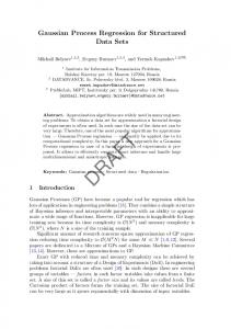
For Laplace’s method, the order of the error ranges from to at the cost of complexity from to as shown in Table I. , which For the Monte Carlo estimators, we introduce is the probabilistic error order and it implies that the estimation error converges to in distribution as the number of random samples increases. Therefore it is not appropriate to compare the error bound between Monte Carlo and Laplace’s method exactly. Monte Carlo algorithms are used for multi. The probabilistic error variate integration of dimension order of Monte Carlo algorithms that use sample evaluations for a given . We may assume that the order of is of order the error for Monte Carlo methods do not depend on the number of measurements for a large [36]. With this assumption, the number of samples needed for Monte Carlo algorithms to reduce is of order . The the initial probabilistic error by complexity of the Monte Carlo methods, for the investigated . To achieve the probabilistic problems in this paper, is , the complexity of Monte Carlo methods error order has to be . If we want to keep the error order at the level of and for Laplace’s and Monte Carlo methods, respectively, the Monte Carlo methods are slightly more expensive than Laplace’s method. VII. SIMULATION RESULTS In this section, we provide simulation results to evaluate the performances of different estimation methods. To this end, a realization of a Gaussian process that will serve as ground truth is shown in Fig. 2. The Gaussian process is generated for and in (1). The measurement noise and the sampling position uncertainty variance are and , respectively. and imply that 20 robot takes measurements twice at each sampling position. In Figs. 2–7, the predicted fields and predicted error variance fields are shown with color bars. The results from Gaussian process regression using the noiseless positions and the noisy measurement are shown in Fig. 3.


Fig. 3. Gaussian process regression using the true positions . a) The predictive mean estimation. b) The predictive variance estimation, and the true sampling positions in aquamarine crosses.

Fig. 4. The results of the QDS 1 approximations using . a) The predictive mean estimation. b) The predictive variance estimation, and shown with aquamarine crosses.

To compare with typical quick-and-dirty solutions (QDS) to deal with noisy locations in practice, we define two solutions: QDS 1 and 2 approaches. QDS 1 is to applying Gaussian process regression given by (3) and (4) by simply ignoring noises in the locations and taking as the true positions, i.e., (32) When the measurements are taken repeatedly as suggested in Section III, QDS 1 could be improved. In this regard, QDS 2 is to use the conditional expectation of sampling positions given as in (19) and the least squares solution of for given , which shall be plugged into Gaussian process regression, i.e., (33)

231

Fig. 5. The results of the QDS 2 approximations using . a) The predicshown tive mean estimation. b) The predictive variance estimation, and with aquamarine crosses.

Fig. 6. The results of the Monte Carlo approximations with 1000 samples using . a) The predictive mean estimation. b) The predictive variance estimation, and shown with aquamarine crosses.

where is from (19) and is from (18). QDS 2 might be an improved version of QDS 1 when there are many repeated measurements for a set of fixed sampling positions. Figs. 4 and 5 show the results of applying QDS 1 and QDS 2 on and , respectively. This averaging helps the QDS approach to generate smoother predictions, and it shows improvement with respect to QDS 1. samThe results of the Monte Carlo method with ples are shown in Fig. 6. The results of Laplace’s method are shown in Fig. 7, and they look very similar to those of the Monte Carlo methods in Fig. 6. Figs. 4–7 clearly shows that both the Monte Carlo and Laplace’s method outperform QDS 1 and 2 with respect to the true field in Fig. 3.

232


we know the true realization of the Gaussian process exactly in this simulation study. As expected, Gaussian process regression with the true locations perform best. The proposed approaches, i.e., Monte Carlo and Laplace’s method outperform QDS 1 and 2 in terms of RMS errors as well. VIII. EXPERIMENTAL RESULTS A. Experiment With Simulated Noisy Sampling Positions

Fig. 7. The results of the Laplace approximations using . a) Predictive mean estimation. b) The predictive variance estimation, and shown with aquamarine crosses.

Fig. 8. The results of the simple Laplace approximations using . a) The predictive mean estimation. b) The predictive variance estimation, and shown with aquamarine crosses. is the estimation of the true sampling positions, computed as a by-product of both fully exponential Laplace and simple Laplace approximations. TABLE II SIMULATION RMS ERROR

To numerically quantify the performance of each approach, we have computed the root mean square (RMS) error between the predicted and true fields for all methods, which are summarized in Table II. This RMS error analysis could be done since

In this section, we apply proposed prediction algorithms to a real experimental data set to model the concentration of , , 24-trihydroxy- -cholan-3-one 24-sulfate (3 kPZS), a synthesized sea lamprey (Petromyzon marinus) mating pheromone, in the Ocqueoc River, MI, USA which the authors of [38] provided. The sea lamprey is an ecologically damaging vertebrate invasive fish invader of the Laurentian Great Lakes [39] and a sea lamprey management program has been established [40]. A recent study by Johnson et al. [38] showed that synthesized 3 kPZS, a synthesized component of the male mating pheromone, when released into a stream to reach (molar) or mol/L, triggers concentrations of robust upstream movement in ovulated females drawing 50% into baited traps. The ability to predict 3 kPZS concentration at any location and time with a predicted uncertainty level would allow for fine-scale evaluations of hypothesized sea lamprey chemo-orientation mechanisms such as odor-conditioned rheotaxis [38]. Here 3 kPZS was added to the stream to produce pulsing excitation to sea lampreys by applying 3 kPZS at two minutes intervals [41]. To describe 3 kPZS concentration throughout the experimental stream, rhodamine dye (Turner Designs, Rhodamine WT, Sunnyale, CA, USA) was applied at the pheromone release point (or source location) to reach a final in-stream concentration of 1.0 mug/L (measure the concentration of the 3 kPZS). The same pulsing strategy is used when 3 kPZS was applied. The dye and 2 kPZS pumping systems are shown in Fig. 9(a). An example of the highly visible dye plume near the source location is shown in Fig. 9(c). To quantify dye concentrations in the stream, water samples were collected along transects occurring every 5 m from the sea lamprey release cage (0 m) to the application location (73 m upstream of release cage) as shown in Fig. 9(b). Three sampling locations were fixed along each transect at 1/4, 1/2 and 3/4ths the channel width from the left bank. Water was collected from the three sampling sites along a transect simultaneously (three samplers) every 10 sec. for 2 minutes time interval. Further, a series of samples over 2 min were collected exactly 1 meter downstream of the dye application location. Water samples were collected in 5 ml glass vials and subsequently the fluorescence intensity of each sample measured at 556 nm was determined in a luminescence spectrometer (Perkin Elmer LSS55, Downers Grove, IL, USA) and rhodamine concentration was estimated . using a standard curve The objective here is to predict the spatio-temporal field of the dye concentration. In fact, the sampling positions are exactly known from the experiment. Therefore, we will intentionally inject some noises in the sampling positions to evaluate the proposed prediction algorithms in this paper. Before applying the proposed algorithms, the hyperparameters such as and


233

Fig. 10. The results of Gaussian process regression using true . a) The posterior mean estimation. b) The posterior variance estimation, and shown with aquamarine crosses.

We consider the anisotropic covariance function [16] to deal with the case that the correlations along different directions in are different. Next, we performed a change of variables such that in a transformed space and time. The covariance function, given (1), could be used for the proposed approaches. For the case of this experiment, the spatial correlation along the river flow direction is different from the correlation perpendicular to the river flow direction. We consider the following covariance function in the units for the experimental data. (34) Using this covariance function in (34) and computing likelihood function with true value of , the hyperparameter vector can be computed by the MAP estimator as follow: (35) , Using the optimization in (35), we obtained and . and are the coordinates of the vertical and horizontal (flow direction) axes of Fig. 10. As , i.e., the field is more correlated we expect, we have along the river flow direction as compared to the perpendicular to the river flow direction. Next, after finding MAP estimates and , we change the scale of each of hyperparameters component of , such that we have the same values for hyperparameters in the transformed coordinates. The new coordinates are given by and we recover

Fig. 9. (a) The dye pumping system. (b) An example of normal dye concentration applied to the stream for the pheromone distribution estimation. (c) An example of the highly visible dye plume near the source location.

were identified from the experimental data by a maximum a posteriori probability (MAP) estimator as described in [16]. On the was set to other hand, the value for according to the noise level from the data sheet of the sensor.

as in (1). Note that scaling with , also transforms the covariance matrix in a normalized space. Table III shows parameter values which are estimated and used for the experimental data. Fig. 10 shows the predicted field by applying Gaussian process regression on the true positions . To illustrate the advantage of proposed methods over the QDS approach in

234


TABLE III EXPERIMENT PARAMETERS

Fig. 13. The results of the Laplace method using noise augmented positions shown with aquamarine crosses. a) The predictive mean estimation. b) The predictive variance estimation and shown with aquamarine crosses.

Fig. 11. The results of the QDS 1 approach using noisy positions . a) The predictive mean estimation. b) The predictive variance estimation, and shown with aquamarine crosses. Fig. 14. The results of the simple Laplace method using noise augmented positions shown with aquamarine crosses. a) The predictive mean estimation. b) The predictive variance estimation and shown with aquamarine crosses.

TABLE IV EXPERIMENTAL RMS ERROR W.R.T. GAUSSIAN ESTIMATION

Fig. 12. The results of the Monte Carlo method with 1000 samples using noisy positions . a) The predictive mean estimation. b) The predictive variance estimation, and shown with aquamarine crosses.

dealing with the noisy localizations, we show the results of applying QDS 1, Monte Carlo, Laplace, and simple Laplace approximations in Figs. 11, 12, 13, and 14, respectively. Since there is only one measurement per position, QDS 2 is same as QDS 1. As can be seen in these figures, the peaks of the predicted fields by Monte Carlo and Laplace’s method with noisy are closer to the peak predicted by the true than that of the QDS approach. Indeed, QDS 1 has failed in Fig. 11 to produce a good estimation of the true field with neglecting the uncertainty in the positions, while Monte Carlo, Laplace and simple Laplace methods, proposed in this paper, produce good estimations in Figs. 12, 13, and 14, respectively. Gaussian regression using true is our best estimation of the true field (Fig. 10). Table IV shows the RMS errors of the different estimation approaches using the noisy (i.e. ) with respect to Gaussian regression using the true . As can be seen in Table IV, the proposed approaches outperform QDS 1 in terms of the RMS error.

B. Experiment With Noisy Sampling Positions In Section VIII-A we used the true and simulated noisy sampling positions to compare the performance of the proposed approaches. In this section, we present another set of experimental results under real localization errors. The experimental results were obtained using a single aquatic surface robot in an outdoor swimming pool as shown in Fig. 15. The robot is capable of monitoring the water temperature in an autonomous manner while could be remotely supervised by a central station as well. To measure the location of the robot, we used a Xsense MTi-G sensory unit [42] (as shown in the center of Fig. 15(a)) which consists of an accelerometer, a gyroscope, a magnetometer, and a Global Positioning System (GPS) unit. A Kalman filter is implemented inside of this sensor by the company, which produces the localization of the robot with accuracy of one meter. More information about this experiment can be found in [43]. In this experiment, we have selected and identified the system parameters based on a priori knowledge about the process and sensor noise characteristics. Therefore, model hyperparameters such as , , , and are known. The number of sampling positions and sampled measurements are . To validate our approaches, we have controlled


235

Fig. 17. The results of the Monte Carlo method with 1000 samples using noisy positions . a) The predictive mean estimation. b) The predictive variance estimation, and shown with aquamarine crosses. Fig. 15. a) The developed robotic sensor. b) The experimental environment- a 12 6 meters outdoor swimming pool.

Fig. 18. The results of the Laplace approximations using . a) Predictive mean estimation. b) The predictive variance estimation, and shown with aquamarine crosses. Fig. 16. The results of the QDS 1 approach using noisy positions . a) The predictive mean estimation. b) The predictive variance estimation, and shown with aquamarine crosses.

the temperature field by turning the hot water pump on and off. The hot water outlet locations have been shown in Fig. 15(b). We turned on the hot water pump for a while. After that, the hot water pump was turned off, and after 6 minutes, the robot collected 10 measurements with 10 sec. time intervals. The estimated temperature and its error variance fields, by applying QDS 1, Monte Carlo, fully exponential Laplace, and simple Laplace methods are shown in Figs. 16, 17, 18, and 19,

respectively. For each method, the estimated temperature and its error variance fields are shown in subfigures of (a) and (b), respectively. As can be seen in Figs. 17, 18, and 19, results from Monte Carlo, fully exponential Laplace, and simple Laplace methods are well matched. IX. CONCLUSION We have formulated Gaussian process regression with observations under the localization uncertainty due to (possibly mobile) sensor networks with limited resources. Effects of the mea-

236


A.5

and

where

. REFERENCES

Fig. 19. The results of the simple Laplace method using noise augmented positions shown with aquamarine crosses. a) The predictive mean estimation. b) The predictive variance estimation and shown with aquamarine crosses.

surements noise, localization uncertainty, and prior distributions have been all correctly incorporated in the posterior predictive statistics in a Bayesian approach. We have reviewed the Monte Carlo sampling and Laplace’s method, which have been applied to compute the analytically intractable posterior predictive statistics of the Gaussian processes with localization uncertainty. The approximation error and complexity of all the proposed approaches have been analyzed. In particular, we have provided tradeoffs between the error and complexity of Laplace approximations and their different degrees such that one can choose a tradeoff taking into account the performance requirements and computation complexity due to the resource-constrained sensor network. Simulation study demonstrated that the proposed approaches perform much better than approaches without considering the localization uncertainty properly. Finally, we applied the proposed approaches on the experimentally collected real data to provide proof of concept tests and evaluation of the proposed schemes in practice. From both simulation and experimental results, the proposed methods outperformed the quick-and-dirty solutions often used in practice. APPENDIX A. Regularity Conditions In this section, we review a set of regularity conditions [26]. denote the open ball of radius centered at , i.e., Let . Let be the asymptotic . The followings are regularity conditions. mode of order . A.1 A.2 . A.3 , for all and all with , where . is positive definite and A.4 .

[1] D. Culler, D. Estrin, and M. Srivastava, “Guest editors’ introduction: Overview of sensor networks,” Computer, vol. 37, no. 8, pp. 41–49, Aug. 2004. [2] D. Estrin, D. Culler, K. Pister, and G. Sukhatme, “Connecting the physical world with pervasive networks,” Pervasive Comput., vol. 1, no. 1, pp. 59–69, 2002. [3] K. M. Lynch, I. B. Schwartz, P. Yang, and R. A. Freeman, “Decentralized environmental modeling by mobile sensor networks,” IEEE Trans. Robot., vol. 24, no. 3, pp. 710–724, Jun. 2008. [4] J. Choi, S. Oh, and R. Horowitz, “Distributed learning and cooperative control for multi-agent systems,” Automatica, vol. 45, pp. 2802–2814, 2009. [5] J. Cortés, “Distributed Kriged Kalman filter for spatial estimation,” IEEE Trans. Autom. Control, vol. 54, no. 12, pp. 2816–2827, 2010. [6] N. Cressie, “Kriging nonstationary data,” J. Amer. Statist. Assoc., vol. 81, no. 395, pp. 625–634, 1986. [7] C. E. Rasmussen and C. K. I. Williams, Gaussian Processes for Machine Learning. Cambridge, MA: MIT Press, 2006. [8] A. Krause, C. Guestrin, A. Gupta, and J. Kleinberg, “Near-optimal sensor placements: Maximizing information while minimizing communication cost,” in Proc. ACM 5th Int. Conf. Inf. Process. Sensor Netw., 2006, pp. 2–10. [9] A. Krause, A. Singh, and C. Guestrin, “Near-optimal sensor placements in Gaussian processes: Theory, efficient algorithms and empirical studies,” J. Mach. Learn. Res., vol. 9, pp. 235–284, 2008. [10] Y. Xu, J. Choi, and S. Oh, “Mobile sensor network coordination using Gaussian processes with truncated observations,” IEEE Trans. Robot., vol. 27, no. 6, pp. 1118–1131, 2011. [11] K. Ho, “Alleviating sensor position error in source localization using calibration emitters at inaccurate locations,” IEEE Trans. Signal Procesd., vol. 58, no. 1, pp. 67–83, 2010. [12] L. Hu and D. Evans, “Localization for mobile sensor networks,” in Proc. ACM 10th Annu. Int. Conf. Mobile Comput. Netw., 2004, pp. 45–57. [13] P. Oguz-Ekim, J. Gomes, J. Xavier, and P. Oliveira, “Robust localization of nodes and time-recursive tracking in sensor networks using noisy range measurements,” IEEE Trans. Signal Process., vol. 59, no. 8, pp. 3930–3942, 2011. [14] R. Karlsson and F. Gustafsson, “Bayesian surface and underwater navigation,” IEEE Trans. Signal Process., vol. 54, no. 11, pp. 4204–4213, 2006. [15] D. Titterton and J. Weston, Strapdown Inertial Navigation Technology. Stevenage, U.K.: Peregrinus, 2004. [16] Y. Xu and J. Choi, “Adaptive sampling for learning Gaussian processes using mobile sensor networks,” Sensors, vol. 11, no. 3, pp. 3051–3066, 2011. [17] M. Mysorewala, D. Popa, and F. Lewis, “Multi-scale adaptive sampling with mobile agents for mapping of forest fires,” J. Intell. Robot. Syst., vol. 54, no. 4, pp. 535–565, 2009. [18] A. Girard, C. Rasmussen, J. Candela, and R. Murray-Smith, “Gaussian process priors with uncertain inputs-application to multiple-step ahead time series forecasting,” Adv. Neural Inf. Process. Syst., pp. 545–552, 2003. [19] J. Kocijan, R. Murray-Smith, C. Rasmussen, and B. Likar, “Predictive control with Gaussian process models,” in Proc. IEEE EUROCON, 2003, vol. 1, pp. 352–356. [20] R. Murray-Smith, D. Sbarbaro, C. Rasmussen, and A. Girard, “Adaptive, cautious, predictive control with Gaussian process priors,” in Proc. 13th IFAC Symp. Syst. Identification, Rotterdam, The Netherlands, 2003, pp. 1195–1200. [21] M. Deisenroth, C. Rasmussen, and J. Peters, “Gaussian process dynamic programming,” Neurocomput., vol. 72, no. 7–9, pp. 1508–1524, 2009. [22] D. Nash and M. Hannah, “Using Monte-Carlo simulations and Bayesian Networks to quantify and demonstrate the impact of fertiliser best management practices,” Environ. Modelling Softw., vol. 26, no. 9, pp. 1079–1088, 2011. [23] M. Wainwright and M. Jordan, “Graphical models, exponential families, and variational inference,” Found. Trends Mach. Learn., vol. 1, no. 1–2, pp. 1–305, 2008.


[24] L. Tierney and J. Kadane, “Accurate approximations for posterior moments and marginal densities,” J. Amer. Statist. Assoc., vol. 81, no. 393, pp. 82–86, 1986. [25] L. Tierney, R. Kass, and J. Kadane, “Fully exponential Laplace approximations to expectations and variances of nonpositive functions,” J. Amer. Statist. Assoc., vol. 84, no. 407, pp. 710–716, 1989. [26] Y. Miyata, “Fully exponential Laplace approximations using asymptotic modes,” J. Amer. Statist. Assoc., vol. 99, no. 468, pp. 1037–1049, 2004. [27] Y. Miyata, “Laplace approximations to means and variances with asymptotic modes,” J. Statist. Planning Inference, vol. 140, no. 2, pp. 382–392, 2010. [28] M. Jadaliha, Y. Xu, and J. Choi, “Gaussian process regression using Laplace approximations under localization uncertainty,” in Proc. Amer. Control Conf., Montreal, QC, Canada, Jun. 27–29, 2012, pp. 1394–1399. [29] A. J. Smola and P. L. Bartlett, “Sparse greedy Gaussian process regression,” in Proc. Adv. Neural Inf. Process. Syst., 2001, vol. 13, pp. 619–625. [30] C. Williams and M. Seeger, “Using the Nystrom method to speed up kernel machines,” in Proc. Adv. Neural Inf. Process. Syst., 2001, vol. 13, pp. 682–688. [31] N. Lawrence, M. Seeger, and R. Herbrich, “Fast sparse Gaussian process methods: The informative vector machine,” in Proc. Adv. Neural Inf. Process. Syst., 2003, pp. 625–632. [32] M. Seeger, “Bayesian Gaussian process models: PAC-Bayesian generalisation error bounds and sparse approximations,” Ph.D. dissertation, School of Informatics, Univ. of Edinburgh, Edinburgh, U.K., 2003. [33] V. Tresp, “A Bayesian committee machine,” Neural Comput., vol. 12, no. 11, pp. 2719–2741, 2000. [34] A. Brix and P. Diggle, “Spatiotemporal prediction for log-Gaussian Cox processes,” J. Roy. Statist. Soc.: Series B (Statist. Methodol.), vol. 63, no. 4, pp. 823–841, 2001. [35] C. Andrieu, N. De Freitas, A. Doucet, and M. Jordan, “An introduction to MCMC for machine learning,” Mach. Learn., vol. 50, no. 1, pp. 5–43, 2003. [36] J. Geweke, “Bayesian inference in econometric models using Monte Carlo integration,” Econometrica: J. Econometric Soc., vol. 57, no. 6, pp. 1317–1339, 1989. [37] H. Durrant-Whyte and T. Bailey, “Simultaneous localisation and mapping (SLAM): Part I the essential algorithms,” Robot. Autom. Mag., vol. 13, no. 2, pp. 99–110, 2006. [38] N. Johnson, S. Yun, H. Thompson, C. Brant, and W. Li, “A synthesized pheromone induces upstream movement in female sea lamprey and summons them into traps,” Proc. Nat. Acad. Sci., vol. 106, no. 4, p. 1021, 2009. [39] B. Smith and J. Tibbles, “Sea lamprey (petromyzon marinus) in lakes huron, michigan, and superior: History of invasion and control, 1936–78,” Can. J. Fisheries Aquatic Sci., vol. 37, no. 11, pp. 1780–1801, 1980. [40] G. Christie and C. Goddard, “Sea lamprey international symposium (slis ii): Advances in the integrated management of sea lamprey in the great lakes,” J. Great Lakes Res., vol. 29, pp. 1–14, 2003. [41] N. Johnson, M. Luehring, M. Siefkes, and W. Li, “Mating pheromone reception and induced behavior in ovulating female sea lampreys,” N. Amer. J. Fisheries Manage., vol. 26, no. 1, pp. 88–96, 2006. [42] Xsens Company, MTi-G, Miniature AHRS With Integreted GPS, 2009 [Online]. Available: http://www.xsens.com/images/stories/products/PDF_Brochures/mti-g leaflet.pdf [43] M. Jadaliha and J. Choi, “Environmental monitoring using autonomous aquatic robots: Sampling algorithms and experiments,” IEEE Trans. Control Syst. Technol., 2012, Preprint, DOI: 10.1109/TCST.2012.2190070.

Mahdi Jadaliha received the B.S. degree in electrical engineering from Iran University of Science and Technology, Tehran, Iran, in 2005 and the M.S. degree in electrical engineering from Sharif University of Technology, Tehran, Iran, in 2007. Currently, he is working toward the Ph.D. degree in mechanical engineering at Michigan State University, East Lansing, under the guidance of Prof. J. Choi. His research interests include statistical learning and system identification, with applications to mobile robotic sensors and SLAM.

237

Mr. Jadaliha’s paper was a finalist for the Best Student Paper Award at the Dynamic System and Control Conference (DSCC) 2012.

Yunfei Xu received the B.S. and M.S. degrees in automotive engineering from Tsinghua University, Beijing, China, in 2004 and 2007, respectively, and the Ph.D. degree in mechanical engineering from Michigan State University, East Lansing, in 2011. Currently, he is a Postdoctoral Researcher in the Department of Mechanical Engineering at Michigan State University. His current research interests include environmental adaptive sampling algorithms, Gaussian processes, and statistical learning algorithms with applications to robotics and mobile sensor networks.

Jongeun Choi received the B.S. degree in mechanical design and production engineering from Yonsei University, Seoul, Republic of Korea, in 1998 and the M.S. and Ph.D. degrees in mechanical engineering from the University of California at Berkeley in 2002 and 2006, respectively. He is currently an Associate Professor with the Department of Mechanical Engineering and the Department of Electrical and Computer Engineering at Michigan State University. East Lansing. His research interests include systems and control, system identification, and Bayesian inference, with applications to mobile robots, environmental adaptive sampling, engine control, and biomedical problems. Dr. Choi was a recipient of an NSF CAREER Award in 2009. His papers were finalists for the Best Student Paper Award at the Twenty-Fourth American Control Conference (ACC) 2005 and the Dynamic System and Control Conference (DSCC) 2011 and 2012. He is a member of ASME.

Nicholas S. Johnson received the B.S. degree in fisheries/limnology and biology from the University of Wisconsin, Stevens Point, in 2004 and the M.S. and Ph.D. degrees in fisheries and wildlife from Michigan State University, East Lansing, in 2005 and 2008, respectively. He is currently a Research Ecologist with the United States Geological Survey, Great Lakes Science Center, Hammond Bay Biological Station, and Adjunct Assistant Professor in the Department of Fisheries and Wildlife at Michigan State University. His research interests include behavioral and chemical ecology of fishes and specifically how to use chemical and electrical stimuli to aid restoration of valued fishes and control of invasive fishes.

Weiming Li received the B.S. degree in aquaculture and the M.S. degree in fish physiology from Shanghai Ocean University, Shanghai, China, in 1982 and 1987, respectively, and the Ph.D. degree in fisheries from the University of Minnesota at Twin Cities in 1994. He is a Professor and FEJ Fry Chair in Environmental Physiology in the Departments of Fisheries and Wildlife and of Physiology at Michigan State University, East Lansing, where he is also a faculty member of the Neuroscience Program and the Ecology, Evolutionary Biology and Behavior Program. His research interests include chemical ecology, physiology of olfaction and endocrine systems, and genomics.