Accepted Manuscript Adaptive Gaussian process regression as an alternative to FEM for prediction of stress intensity factor to assess fatigue degradation in offshore pipeline Arvind Keprate, R.M. Chandima Ratnayake, Shankar Sankararaman PII:
S0308-0161(17)30046-7
DOI:
10.1016/j.ijpvp.2017.05.010
Reference:
IPVP 3619
To appear in:
International Journal of Pressure Vessels and Piping
Received Date: 30 January 2017 Revised Date:
4 May 2017
Accepted Date: 9 May 2017
Please cite this article as: Keprate A, Ratnayake RMC, Sankararaman S, Adaptive Gaussian process regression as an alternative to FEM for prediction of stress intensity factor to assess fatigue degradation in offshore pipeline, International Journal of Pressure Vessels and Piping (2017), doi: 10.1016/ j.ijpvp.2017.05.010. This is a PDF file of an unedited manuscript that has been accepted for publication. As a service to our customers we are providing this early version of the manuscript. The manuscript will undergo copyediting, typesetting, and review of the resulting proof before it is published in its final form. Please note that during the production process errors may be discovered which could affect the content, and all legal disclaimers that apply to the journal pertain.
ACCEPTED MANUSCRIPT
Adaptive Gaussian process regression as an alternative to FEM for prediction of stress intensity factor to assess fatigue degradation in offshore pipeline Arvind Keprate*1
Shankar Sankararaman2
Department of Mechanical & Structural Engineering and Materials Science, University of Stavanger, N-4036, Norway 2 SGT Inc., NASA Ames Research Center, Moffett Field, CA 94035, USA
RI PT
1
R.M. Chandima Ratnayake1
Abstract
The linear elastic fracture mechanics (LEFM) based remnant fatigue life (RFL) assessment of offshore pipeline is used to determine the inspection interval frequency of the aforementioned asset. One of the vital factors of the LEFM approach that determines the accuracy of the RFL estimate (and in turn of the inspection
SC
interval frequency) is the Stress Intensity Factor (SIF), which must be evaluated as accurately as possible. For simple crack geometries numerous closed-form equations available in various handbooks and industrial standards provide accurate SIF results. However, it is a common industry practice to utilize finite element
M AN U
method (FEM) for evaluating the SIF for the intricate crack geometries and the complex loading conditions. Although, FEM is known for its accurate SIF calculation, but due to its high computational expense and timeconsumption, cycle-by-cycle SIF evaluation (required for the LEFM based RFL assessment) makes the aforementioned method quite laborious. Furthermore, using FEM to evaluate SIF for thousands of pipeline location (undergoing fatigue degradation) on an offshore platform seems to be impractical. Thus, in this manuscript authors have proposed a computationally inexpensive adaptive Gaussian process regression model
TE D
(AGPRM) which may be utilized as an alternative to FEM for prediction of SIF to assess fatigue degradation in offshore pipeline. The training and testing data for AGPRM consists of 105 and 50 data points (load (L), crack depth (a), half-crack length (c) and SIF values), respectively. Latin Hypercube Sampling (LHS) is used to generate (L, a and c) values while SIF values are evaluated using FEM by carefully accounting for the
EP
discretization error emanating due to the finite mesh size in the FEM simulation. After the GPRM has been adaptively trained, it is used to predict the response of the 50 data points. On comparing the values of the SIF
AC C
(obtained by AGPRM) with the SIF values obtained from FEM, the average residual percentage between the two is found to be 1.76%, thus indicating a good agreement between the AGPRM and FEM model. Furthermore, the time required to predict the SIF of 50 test points is reduced from 50 minutes (for FEM) to 12 seconds with the help of the proposed AGPRM, thus making RFL assessment less laborious and time consuming.
Keywords: Adaptive Gaussian process regression model, FEM, SIF, offshore pipeline, Fatigue
1. Introduction 1.1 Background During its service life, topside pipeline on offshore oil and gas platforms is continuously subjected to vibrations emanating from various excitation sources such as flow induced turbulence, flow induced pulsation,
1
ACCEPTED MANUSCRIPT * Corresponding author: Tel.: +47 40386776 E-mail address:
[email protected] mechanical excitation, acoustic induced vibrations etc. [1]. Due to the aforementioned vibrations, dynamic stresses are induced in the pipework, which if above threshold level, may lead to fatigue crack initiation and propagation in the vibrating pipeline [2]. In order to assure that the propagating crack does not cause failure of topside pipeline during its service life, it is vital to perform Remnant Fatigue Life (RFL) assessment of the
RI PT
aforementioned asset. The results of the RFL assessment must demonstrate that probability of failure (PoF) of topside pipeline due to fatigue cracking remains within the target levels set by an operator [3]. In case, the PoF crosses above the threshold level, an in-service inspection is recommended. While, the first inspection interval is decided on the basis of RFL calculated using the stress-life (S-N) approach, the subsequent
SC
inspection interval rely on the RFL evaluated using the linear elastic fracture mechanics (LEFM) approach coupled with probabilistic analysis [3].
The basis of the LEFM approach, lies in performing a cycle-by-cycle crack propagation analysis (CPA),
M AN U
using a suitable crack growth law (such as Paris equation, Forman equation, etc.,) on an initial crack size (ICS) to determine the number of cycles required for an ICS to reach critical crack size (CCS) [4]. Thus, RFL assessment using LEFM approach is mainly dependent upon two factors namely: ICS and crack growth law. In regards to the first factor, BS7910 [5] recommends that the value of ICS should be determined by the detection threshold limit of the NDE method (for instance ICS based on detection limit of UT is 1.5mm). Nevertheless, authors have highlighted the disadvantages of ICS derived from NDE detection threshold in [6]
TE D
and hence proposed using Equivalent Initial Flaw Size (EIFS) concept which depends on material properties (i.e. threshold stress intensity factor and endurance limit) and geometric function (Y) to determine ICS [6]. The advantages of EIFS approach is discussed by authors in [6]. The second important factor for LEFM based RFL assessment is a suitable crack growth law which
EP
calculates the crack growth increment per cycle (i. e. domain is Paris equation, according to which
). Most commonly used crack growth law in LEFM
is directly proportional to the SIF (which relies upon nominal
AC C
stress, Y and crack size (a)), at the crack tip of the propagating crack [7, 8]. Thus, once
is evaluated for the
first cycle it is added to the ICS in order to obtain crack size at first cycle. In this way, the entire process is iterated until ICS reaches CCS and the number of cycles required to do so represents the RFL, which may then be used to decide inspection interval frequency for topside pipeline. Consequently, based on the aforementioned discussion it is affirmed that the accuracy of the RFL estimate (and in turn of the inspection interval frequency) depends upon accurate evaluation of the SIF. At present, SIF evaluation is possible through several methods such as handbook solutions [9, 10, and 11], analytical methods (e.g. conformal mapping, body force), experimental methods (fatigue crack growth, interferometry, etc.) and numerical methods (finite element method (FEM), boundary collocation techniques, etc.). Readers interested in gaining more insight into SIF determination methods may refer to [12 and 13].
2
ACCEPTED MANUSCRIPT Usually, handbook solutions give accurate SIF results for simple crack geometries [13]. However, as the intricacy of crack geometry and the complexity of the loading augments, handbook solutions are not the best way to evaluate SIF [14]. Consequently, under such circumstances, analysts use tools such as FEM for SIF evaluation [15]. In the past, researchers such as Bergman and Brickstad [16], Zahoor [17], Zareei and Nabavi [18], Miyazaki and Mochizuki [19], and Kumar et al., [20] have used FEM to determine the SIF of cracks propagating in pipes. Nevertheless, FEM techniques are afflicted with the following constraints:
RI PT
1. The accuracy and computing time required to solve a FEM simulation is dependent upon the finite element size (mesh density). This implies that simulations of finite element models constructed with fine mesh size deliver accurate results, nevertheless the simulations generally take longer computing time and vice-versa [21].
SC
2. Generally, three types of error are attributed to FEM, namely: user error (which emanates due to inexperience of the analyst), modeling error (which arises due to erroneous representation of the real world phenomenon) and discretization error (originating due to inadequate mesh density which is unable to capture
M AN U
the solution appropriately) [22]. While the former two errors are in the hands of the analyst, the latter is inherent to FEM and must be separately quantified by the analyst for an accurate solution. Thus, quantification of discretization error increases the accuracy of FEM results; however, it further adds to the time required to run a FEM simulation.
Based on the above mentioned two points, it is deduced that the higher accuracy in the SIF evaluated through FEM is achieved at the expense of the greater time required for simulations to run, which makes FEM
TE D
computationally expensive and time-consuming. The aforementioned shortcoming of FEM causes hindrance while performing LEFM based RFL assessment of offshore pipeline in the following two ways: 1.
In real life the number of FEM simulations required to predict the SIF for cycle-by-cycle CPA
is of the order of 10 or more. Hence, if for one FEM simulation thirty seconds are required to evaluate the
EP
SIF, then approximately a month will be required to predict SIF for 10 cycles, thus making RFL assessment using FEM quite laborious and uneconomical.
On an offshore platform, there could be more than thousands of pipeline locations (in
AC C
2.
particular small bore connections) undergoing fatigue degradation. Performing the LEFM based RFL assessment by evaluating the SIF (using FEM) for thousands of pipeline locations is practically impossible.
In order to overcome the aforementioned shortcomings of FEM, in evaluating the SIF for RFL assessment of topside pipeline, it seems more efficient and rational to design and run a limited number of FEM simulations (with small element size and for which the discretization error has been accounted for), that act as the training and testing points for a metamodel (MM), which in turn is used to predict the SIF value accurately and instantly at other data points (i.e. (load (L), crack depth (a), half-crack length (c)), thus making RFL assessment of topside pipeline less labor intensive and economical.
3
ACCEPTED MANUSCRIPT 1.2 Metamodels Metamodels (MMs), are a data-driven models that try to emulate the complex input/output (I/O) behavior of underlying system, by using a limited set of computational expensive simulations (CES) [23]. The two basic steps while constructing a MM are training and testing. The first one corresponds to fitting a model to the intelligently chosen training points, while the second step involves comparing the predictions of MM to the actual response [23]. For the readers interested in gaining more insight into complete procedure of
RI PT
constructing a MM, are referred to [23]. The MMs must not be mistaken as a simplified version (with low reliability) of the CES; conversely, MMs emulate the behavior of the CES as accurately as possible, coupled with the low computational cost [24].
At present, MMs are commonly used to replicate the results of a single expensive simulation code that
SC
needs to be run time and again in order to generate the desired results [23]. For such applications, MMs act as a ‘curve fit’ to the training data (generated by expensive simulation code) and thereafter may be used in the future to estimate the quantity of interest without running the expensive simulation code [23]. The main idea
M AN U
of using MMs as a replacement to the original simulation code or program is based on the fact that, once built, the MMs will be faster than the main simulation code, while still being usefully accurate [23]. In the aforementioned context, MMs may be used to predict the SIF of a propagating crack. To date, MMs have been developed for predicting SIF in aluminum in the aeronautical and aerospace industries [24, 25, and 26]. Yuvraj et al. [27] used MM to predict critical SIF for concrete beams. Larrosa et al. [28] have proposed the use of a fitted SIF MM that can be used in LEFM based fatigue life estimations of cracked specimens.
TE D
However, based on the literature review, the authors discovered that, up until now, the commonly used standards for RFL assessment in the offshore industry, i.e. BS 7910 [5], API 579 [28] and DNVGL- RP-C210 [4], rely on either closed-form solutions given in various SIF handbooks or FEM to predict the SIF. Moreover, other than Appendix C of API 579 [29], which uses a third order polynomial equation (which is a type of
EP
MM) along with an influence coefficient to predict SIF, the authors have not come across any other scientific paper or report demonstrating the application of MMs to predict SIF for assessing fatigue degradation of topside pipeline in the offshore industry.
AC C
Building on the literature review, which highlighted the lack of application of MMs to predict the SIF of a crack propagating in offshore pipeline, the authors compared five different MMs, namely multi-linear regression (MLR), second order polynomial regression (PR-2) (with interaction), Gaussian process regression model (GPRM), neural network (NN) and support vector regression (SVR), to predict SIF. The details of the aforementioned comparison can be found in [30]. On the basis of the comparison presented in [30], GPRM was the most apt MM to predict the SIF of a crack propagating in a pipeline component. Thus, the main objective of this manuscript is to present the mathematical background and the procedure for building, adaptive training and testing of the GPRM which may be used to predict SIF in offshore pipeline. In the next section the theory and the procedure to build, adaptively train and test GPRM for SIF evaluation to assess fatigue degradation in offshore pipeline is discussed.
4
ACCEPTED MANUSCRIPT The remainder of the paper is structured as follows. Section 2, elucidates the theory of GPRM coupled with the procedure to build the GPRM. That is followed by the presentation of an illustrative case study in Section 3. Finally, suitable conclusions are made in Section 4.
2. Adaptive Gaussian Process Regression Model 2.1 Introduction
RI PT
A Gaussian Process (GP) is a group of random variables, such that any finite number of it belongs to a joint Gaussian distribution [31]. GP has been used as a general regression model since circa the mid-1970’s; however, in the machine learning domain, the first use of GP took place in 1996 [32]. Gaussian process regression (GPR) is a non-parametric kernel-based stochastic technique, built on the fundamentals of spatial
SC
statistics, that employs a set of observed inputs and outputs to build an approximate model of the underlying relationship [33, 34]. Over the past few years, GPRM has garnered interest amongst the engineering community for its ability to be used as a MM [33]. When used as a MM, the main aim of a GPR model
M AN U
(GPRM) is to use the training data obtained from expensive computer simulation to emulate the underlying relationship and thereafter to use GPRM in the future to estimate the quantity of interest without running expensive simulation code [33]. Furthermore, the core idea of GPRM is that the output values i.e. Y (SIF for our case) assessed at varying values of the input variables i.e. X (L, a, and c for our case), are modeled as a Gaussian random field, with a known mean and covariance function [35]. Some of the advantages of the GPRM are:
1.
TE D
The GPRM is a non-parametric technique, which implies that it does not require a priori
approximation regarding the functional correlation between the input variables and the output variables [33].
2.
The GPRM requires less number of training and testing points when compared to other non-
EP
parametric regression technique such as kernel estimation [35].
3.
The GPRM has the ability to calculate the uncertainty associated with its prediction [33]. This
AC C
uncertainty representation can be quite useful, and shall be used to adaptively train the GPRM. The mathematical background of the GPRM is discussed in the next section.
2.2 Theory
Suppose training points consist of a d-dimensional input variable vector (the input variables being the crack size and loading conditions in our case) stated as ( ), ( ), ( ), … . (
where
is a
,
,….
, and the output random vector
) (the SIF, in this case). It is also possible to write training points as
matrix and
( ) conforming to the input (
evaluated as [35]:
,
is a
vs.
,
1 vector. Now if the analyst wants to predict the output values
), where
is a matrix; then, the joint density output values
5
are
,
,
,
In Eq. (1),
ACCEPTED MANUSCRIPT
̴ !( . ")
(1)
denotes the hyper-parameters of the GP, the value of which is evaluated by the training data.
The prediction mean and covariance matrix (m and S respectively) are given by [35]: + '( ))*
" = $%% − $% ($ In Eq. (2) $
+ '( ))* $
%
is the covariance function matrix (size
) amongst the input training points (
$% is the covariance function matrix (size ) between the input prediction point (
training points (
−
=
SC
,, -;
), and
) and the input
). These covariance matrices are composed of squared exponential terms, where each
element of the matrix is computed as [35]:
$,- = $
(2)
RI PT
= $% ($
(23,4 *24,5 )6 9 [∑:; ] 7 5
M AN U
(3)
/
It must be noted here that all of the above computations require the estimate of the hyper-parameters . The
multiplicative term ( = 1 ?@ ), and the noise standard deviation ('( ) constituting these hyper-parameters
following log-likelihood function [35]:
│
;
=−
CDD
($
+ '( ))*
− log|$
TE D
=@A
and are estimated based on the training data by maximizing the
9
+ '( )| + log (2J)
(4)
Once the hyper-parameters are estimated, then the GPRM can be used for predictions using Eq. (2). A vital issue while constructing the GPRM is how an analyst choses the training points. Usually, the training points
EP
emanate from either the field experiments or using a computer algorithm. In this manuscript, authors have considered the latter case for the generation of training points, due to which the data is noise free, consequently leading to elimination of '( from Eq. (2) and Eq. (4). Furthermore, variance of the predicted follows.
AC C
output will be used later for adaptive training of the GPRM. The procedure used to construct the GPRM
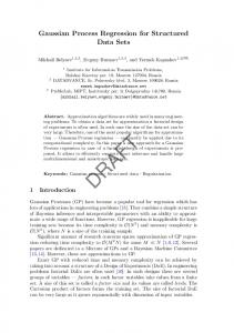
2.3 Steps to Construct Adaptive GPRM The important steps taken to construct an adaptive GPRM are shown in the flowchart depicted in Fig. 1. The individual steps are enumerated in the following sub-sections.
2.3.1 Step 1: Generate Design Space: Three different sets of data (comprising of L, a, and c values), which constitute the design space, are generated using Latin Hypercube Sampling (LHS). The reason for using LHS to generate design space is because of its ability to divide the input distribution into N segments, each of which has an equal probability, and thereby, select one sample from the aforementioned segment [36]. Thus, LHS helps in scattering the training/testing points more evenly across the
6
ACCEPTED MANUSCRIPT design space. The MATLAB algorithm for LHS used for generating the design space is given in Appendix A. The first data set is used for initial training of the GPRM, the second data set is used for testing the GPRM, while the third data set is used to adaptively train the GPRM.
2.3.2 Step 2: Training the GPRM: In context to Fig. 1, the arrows marked as green depict the training of the GPRM. The important steps while training a GPRM are outlined below: 1. Step A: Generate Training Points – As discussed in sub-section 2.3.1, the design space for training
AC C
EP
TE D
M AN U
SC
RI PT
and testing points (i.e. L, a, and c values) is generated using LHS algorithm, as shown in Fig. 1.
7
ACCEPTED MANUSCRIPT Latin Hypercube Sampling to Generate Design Space (i.e. L, a and c Values)
1000 Points (Combination of L, a, c) for adaptive training
50 Testing Points (Combination of L, a , c )
Run FEA to predict SIF for Testing Points. Acccount for Discretization Error in FEA Simulations
M AN U
Final Training Points (L, a, c, SIF)
SC
Run FEA to predict SIF for Training Points. Acccount for Discretization Error in FEA Simulations
RI PT
100 Training Points (Combination of L, a, c )
Final Testing Points (L, a, c, SIF)
Final Testing Points (L, a, c) Values
Gaussian Process Regression (GPR) Model
Final Testing Points (SIF) Values
TE D
Trained GPR Model
EP
Predict Values of Variance for 1000 Combination of L, a, and c
Predict Values of SIF for Each Combination of L, a, and c
Accurate
AC C
Combination (L, a, and c) with Largest Value of Variance
Add One More Training Point (L, a, and c values) No
Yes
Final GPR Model
Fig. 1. Flowchart to build adaptive Gaussian process regression model.
2. Step B: Run FEM Simulation – Once the training points from the design space have been generated, the next step is to perform FEM simulations on the training points (i.e. L, a, and c values) to predict SIF. However, as highlighted in Section 1.1, for an accurate SIF solution, before running FEM simulation, the quantification of the discretization error must be performed by an analyst. In the literature, several methods
8
ACCEPTED MANUSCRIPT [37, 38 and 39] are available to account for the discretization error, but the Richardson extrapolation (RE) [40, 41] method is the most accurate method for quantification of the FEM discretization error and is discussed next. FEA Discretization Error: Let ɛ denote the mesh/element size used in the FEM and µ the corresponding
finite element prediction. Now suppose μL refers to the “true” solution of the FEM which is obtained as ɛ tends to zero. According to the generalized RE [40], the relation between ɛ and µ is written as:
RI PT
μL = μ + CɛO
(5)
In Eq. (5), b is the convergence order, and C is the polynomial coefficient. Since, Eq. (5) has three
unknowns b, C and μL , thus in order to estimate their value we require three mesh solutions. In order to obtain
the true solution μL , three different mesh/element sizes (ɛ < ɛ < ɛ ) are considered and the corresponding
SC
finite element solutions (μ , μ , μ ) are calculated. Even though any three arbitrary mesh/element sizes can be used for solving Eq. (5), however, mesh doubling/halving is commonly done in order to simplify the ɛQ ɛ6
ɛ
= ɛ6 , then the discretization error (eS ) and the true solutions can be calculated as [40]:
μL = μ − eS ; eS =
R
T6 *TR :U *
;
=
Y ZY VWX ( Q R ) Y6 ZYR
VWX (:)
M AN U
equations. If > =
(6)
The solutions μ , μ , μ are dependent on the inputs (L, a and c values) to the FEM and hence the error
estimates are also the functions of these input variables. For each set of inputs, a corresponding discretization
error (eS ) is calculated and this error is subtracted from the finite element solution (using the finest mesh ɛ )
TE D
to estimate the true solution μL [35]. The corrected solutions and the corresponding sets of inputs are used as
training points for the GPRM. Note that the RE method relies only on solutions from multiple mesh densities and does not consider the effects of shape and distribution of elements [35]. Hence, in reality, this is a simple
EP
method that gives an estimate of the discretization error. Other sophisticated methods [42] may be used to calculate the discretization error. The focus of this paper is to demonstrate how the discretization error can be
AC C
included in the construction of GPRM and not to develop accurate methods for the calculation of discretization error.
2.3.3 Step 3: Testing the Trained GPRM: It is in this step that the SIF values of the testing points (L, a, and c values) predicted by the trained GPRM are compared with the SIF values (of the same testing points) generated by FEM. In context to Fig. 1, the arrows marked as brown depict the testing of the GPRM. If the SIF values predicted by GPRM are in agreement with the SIF values evaluated using FEM then the GPRM is considered to be the final version, else adaptive training of the GPRM is performed; an explanation of this follows.
2.3.4 Step 4: Adaptive Training and Testing of the GPRM: Since, GPRM has the capability of estimating the variance in its output values, so a greedy algorithm (GA) which is based on minimization of
9
ACCEPTED MANUSCRIPT variance is used to adaptively train the GPRM [33]. The aforementioned algorithm has twofold advantages, firstly it eradicates the subjectivity related to choosing the training points and secondly it guarantees that the selected training points will minimalize the variance in the GPRM output [33]. Nevertheless, it must be mentioned here that the algorithm used by authors in this manuscript is much more advanced than the GA used by McFarland in [33]. This is because the authors have used three different sets of data points for initial training, testing and adaptive training of GPRM in contrast to McFarland GA which uses a single data set for
RI PT
training and testing. In context to Fig. 1, the arrows marked as red depict the adaptive training of the GPRM to obtain final version of adaptive GPRM (AGPRM). As can be seen from Fig. 1, the algorithm selects the next training point from the 1000 points on the basis of the largest variance and adds it to the previous training points in order to adaptively train the GPRM [35].The algorithm is iterated, and the training points are
SC
identified and added until the estimated variance is below a threshold set by an analyst.
Once the final version of the AGPRM has been created using the aforementioned approach, it may then be
M AN U
used instead of the FEM to predict the SIF for other crack sizes and loading magnitudes during the cycle-bycycle CPA. The next section presents an illustrative case study, which shows the utilization of the AGPRM to predict the SIF of offshore pipeline.
3. Illustrative Case Study 3.1 General
The offshore pipeline material considered for numerical analysis is in accordance with industry practice and
TE D
is assumed to be API5L-Grade B. The authors seek to highlight the fact that, in the present case study, the AGPRM is used to predict the SIF of a semi-elliptical crack at the center of a flat plate; however, the proposed AGPRM can be used to evaluate the SIF for any crack configuration, loading condition and structural geometry (which can be modeled in FEM), since the prediction of the AGPRM depends upon the training and
EP
testing points generated by FEM. Nevertheless, to ease the reader’s understanding, instead of a semi-elliptical crack in a pipe, we have considered a semi-elliptic surface flaw at the center of the flat plate (as depicted in
AC C
Fig. 2) and evaluated the SIF by using three different methods. The aforementioned approximation considered by the authors is supported by the fact that most of the large diameter pipelines used in the O&G sector are manufactured from flat plates using the UOE forming process [43], therefore the SIF solutions for plates may be utilized to approximate the solution for pipes by introducing an appropriate bulging factor [29]. In other words flat plate solution is a good approximation for large diameter pipelines (i.e. thin-walled cylinders) as the hoop stress is constant in the aforementioned asset. The schematic of the plate and crack geometry used in the case study is shown in Fig. 2, while the details of the plate geometry along with its material properties are given in Table 1.
10
ACCEPTED MANUSCRIPT 2c θ
a
A t
RI PT
Le Fig. 2. Schematic of plate and crack geometry.
Table 1. Material and Geometry Properties of API5L-Grade B.
Value
Geometrical Properties
Value
Modulus of Elasticity
210 GPa
Length (Le)
273 mm
Poisson Ratio
0.3
Width
60 mm
Yield Stress/Tensile Stress
241 GPa/350 GPa
Thickness (t)
10 m
M AN U
3.2 SIF Calculation
SC
Material Properties
In this case study, the SIF calculation is performed using three different methods. The first is analytical
AGPRM. 3.2.1
BS7910 Solution
TE D
using the formula given in BS7910 [5], the second is FEM (using ANSYS software) and the third is using
EP
As per BS7910, the SIF can be simply expressed as a function of crack size and loading conditions using a closed-form solution given in Eq. (7).
(7)
AC C
∆$ = ∆' √J]
As geometric function (i.e. parameter Y in Eq. (7)) depends upon the geometry of the component and the crack, so it is a complex function of the crack size and is stated as [5]: = ^ ∗ `a ∗ ^
(8)
In Eq. (8) M is the bulging factor and equals 1 for the flat plate, `a is the finite-width correction factor, and ^ is the factor for membrane loading. `a and ^
are given by Eq. (9) and Eq. (10) respectively:
`a = b(sec( gh ∗ i j ) ef
L
for
11
f
gh
≤ 0.8
(9)
L n
L
ACCEPTED MANUSCRIPT
^ = k^ + ^ l m + ^ l m o ∗ A ∗ `/ /q j j
(10)
The detailed calculation for evaluating Y is given in [6]. Once the value of Y has been calculated, the
next step involves the calculation of SIF using Eq. (7). The resulting values of the SIF for different combinations of loading, crack depth and half crack length (i.e. L, a and c) are shown in Table 5, given in
3.2.2
RI PT
Appendix A.
Finite Element Method
The FEM model of the plate with a semi-elliptical surface crack is shown in Fig. 3 and is constructed using the commercially available software, ANSYS 17 [44]. The damage under consideration is a semi-elliptical fatigue crack (having depth a, and length 2c) in mode-I opening, having its length running perpendicular to
SC
the loading axis. A uniaxial tensile load is applied perpendicular to the crack front i.e. on the smaller sides of the rectangular plate. As can be seen from Fig. 3, different mesh sizes has been used in the analysis, with the
M AN U
mesh around the crack location (at the crack front and surrounding areas) being more refined than rest of the plate geometry. The reason for a finer mesh at the crack location is to obtain a more accurate SIF solution at the crack tip and to avoid convergence problems. Singular elements were used to model the crack tip region. The reason being that stresses and strains are singular at the crack tip. Thus, to produce singularity in the stresses and strains, the elements around the crack tip were modeled using singular elements. Other relevant information related to the FEM is given in Table 2. The reason for using hex dominant element was because when compared to tetrahedron elements, the hex dominant meshing uses significantly less number of elements
TE D
thus making FEM computations faster.
Table 2. FEM details used in the case study.
Parameter Value
Mesh Method
Hex Dominant
EP
Parameter Name
0.2 mm
Crack Front Divisions
15
Circumferential Divisions
8
Mesh Contours
6
Maximum Number of Elements/Nodes
32000
Mesh Size
2.8mm, 5.6mm, 11.2 mm
AC C
Largest Contour Radius
The FEM model is run for data (combination of load, a, and c) obtained using LHS. For the analysis the range of load (L) varies from 100MPa to 200MPa, while the range of crack depth (a) lies between 1mm and 8mm. Likewise, the range of half crack length (c) varies from 2mm to 22mm. For each FEM simulation, the discretization error due to finite mesh size is evaluated and the corrected SIF value in turn is used to train the GPRM. Furthermore, interaction integral method was used to calculate SIF using FEM. Even though three different mesh sizes of 2.8mm, 5.6mm and 11.2mm at the crack tip were used to quantify the discretization
12
ACCEPTED MANUSCRIPT error in this manuscript; however, it is possible to choose any three arbitrary values of the mesh sizes. The reason for choosing the aforementioned mesh sizes is because choosing the mesh size which are double of each other helps in simplification of calculation while estimating the discretization error. The maximum discretization error was found to be 3.48% of the finest mesh solution (i.e. for 2.8mm mesh size). The values of SIF for three different mesh sizes and in turn the corrected SIF value (i.e. one obtained after accounting for
M AN U
SC
aforementioned value of the SIF is used for initial training of the GPRM.
RI PT
discretization error) for 100 training points are shown in Table 3 (given in Appendix A) and in Fig. 4. The
AC C
EP
TE D
Fig. 3. FEM model of the plate and crack geometry used in the case study.
13
M AN U
SC
RI PT
ACCEPTED MANUSCRIPT
Fig. 4. Graph showing values of the SIF for 100 training points.
Gaussian Process Regression Model
TE D
3.2.3
Using the flowchart shown in Fig. 1, the GPRM is initially trained and then used to predict the value of the SIF. In order to investigate the influence of the number of training points on the prediction quality of the GPRM, it is trained firstly by the first 50 data points shown in Table 3 and afterwards by all the 100 data
EP
points of Table 3. Thereafter, the two trained GPRM models (i.e. GPRM-50 (trained by 50 data points) and GPRM-100 (trained by 100 data points)) are used to predict the value of the SIF for the 50 data points shown in Table 4 (Appendix A). The SIF predicted by GPRM-50 and GPRM-100 is then tested against the SIF
AC C
values obtained by ANSYS. The values of the SIF for the 50 data points obtained by GPRM-50, GPRM-100, ANSYS and BS7910 are given in Table 4 and plotted in Fig. 5.
14
M AN U
SC
RI PT
ACCEPTED MANUSCRIPT
3.2.3.1 Result Discussion
TE D
Fig. 5. Graph showing the SIF values predicted by BS7910, ANSYS, GPRM-50 and GPRM-100.
On the basis of the data presented in Fig. 5 and Table 4, the following inferences are made: The value of SIF obtained by using the solution given in BS7910 [5] is always higher than
EP
1.
that obtained from ANSYS. The aforementioned results indicate that the solution given in [5] overestimates the value of the SIF. The reason for the aforesaid overestimation is that the higher value of
AC C
the SIF implies a lower value of RFL of an operating asset, which in turn implies smaller inspection intervals and enhanced process safety [45, 46]. Thus, by overestimating the SIF value, BS7910 provides a conservative estimate of RFL and inspection intervals which is in accordance with the industry practice. 2.
Since the value of the SIF obtained from FEM (i.e. ANSYS) is used to train and test the
GPRM-50 and GPRM-100, it is necessary to measure their accuracy. Generally, in the prognostics domain, the metric used to measure the accuracy of a MM is the residual, which is the difference between the observation and the estimation. Depending upon the field of application, the residual may be estimated in various ways such as, a percentage, a squared quantity, a Euclidian norm, or an amalgamation of the aforementioned [47]. Thereafter, the average of residuals may be used for the assessment of accuracy [47]. In this case study the mean square prediction error (MSPE) is used for accuracy evaluation of the GPRM. The MSPE of GPRM-50 and GPRM-100 was found to be 513.9 and 327.6 respectively,
15
ACCEPTED MANUSCRIPT indicating higher accuracy of GPRM-100. Thus, the aforesaid results indicate that by increasing the number of the training points the prediction accuracy of the GPRM is increased. Henceforth, GPRM-100 will be considered in the case study and shall be adaptively trained to further reduce the prediction error.
3.2.4
Adaptive Gaussian Process Regression Model
In this step the flowchart shown in Fig. 1, is used to construct the Adaptive Gaussian Process Regression
RI PT
Model (AGPRM) which is thereby used to predict the value of the SIF. Initially, GPRM-100-0 (GPRM-100 version 0) is used to predict the variance (s2) of 1000 new data points (generated by LHS) which have not been utilized previously for the training and testing of the GPRM-100-0. Out of the 1000 data points, the data point with the maximum variance (s2) is then chosen, and FEM is used to predict the value of corrected SIF
SC
for this data point. Thereafter, the aforementioned data point is added to the previous training data (consisting of 100 data points). Thus, now we get 101 training points, that are used to train GPRM-100 version 0 (GPRM100-0) in order to get trained GPRM-100 version 1 (GPRM-100-1), which is then used to predict the value of
M AN U
the SIF for the 50 testing data points shown in Table 4. The aforementioned step of the adaptive training is repeated several times until the value of the maximum variance (s2) for data points used for adaptive training (i.e. 1000 L, a, and c values) reaches the threshold value set by the analyst (the authors in this case). For the current case study, the value of the MSPE of the different GPRM-100 versions (varying from 0 to 5) continuously decreases, as shown in Fig. 6. Likewise, the maximum variance (s2) for data points used for adaptive training reaches the threshold of 0.96 (set by the authors) for GPRM-100-5 (as shown in Fig. 7) and
TE D
hence the final GPRM version used for predicting the SIF is GPRM-100-5. Furthermore, the value of the SIF
AC C
EP
predicted by ANSYS, GPRM-100-0 and GPRM-100-5 is shown in Fig. 8 and Table 5.
16
M AN U
SC
RI PT
ACCEPTED MANUSCRIPT
AC C
EP
TE D
Fig. 6. Graph showing relationship between the MSPE (of 50 test points) and the GPRM version.
Fig. 7. Graph showing relationship between the maximum variance (of 1000 points) and the GPRM version.
17
M AN U
SC
RI PT
ACCEPTED MANUSCRIPT
3.2.4.1 Result Discussion
TE D
Fig. 8. Graph showing the SIF values predicted by ANSYS, GPRM-100-0 and GPRM-100-5 (i.e. AGPRM).
On the basis of the data presented in Fig. 6, Fig. 8 and Table 5, the following inferences are made: As indicated by Table 5, the MSPE of GPRM-100-0 is 327.6 while that of GPRM-100-5 is
EP
1.
210.5, indicating the higher prediction accuracy of the adaptively trained GPRM-100-5 version. The benchmark for MSPE is the corrected SIF value obtained from ANSYS. Furthermore, the Maximum
AC C
Absolute Error (MAE) also decreased from 68.57 to 56.49 by adaptively training the GPRM, further indicating the higher accuracy of GPRM-100-5 in comparison to GPRM-100-0. Thus, higher prediction accuracy is achieved by adaptively training the GPRM. 2.
Generally, while selecting a suitable SIF evaluation method, an analyst must consider factors
such as time available, error, cost (includes building and prediction cost), crack geometry, effort required to build the model and effort required to predict the SIF using the model [48]. Thus, Table 6 compares the three methods of SIF determination (i.e. BS7910, ANSYS and AGPRM) used in this case study according to the aforementioned attributes. The comparison for the time consumed to determine the value of the SIF is done on the basis of prediction for the 50 data points shown in Table 5. Furthermore, the value of error for BS7910 (i.e. handbook solution) and FEM has been taken from [48], while the value of error of the AGPRM corresponds to the mean of the absolute percentage difference between the SIF values predicted
18
ACCEPTED MANUSCRIPT by ANSYS and GPRM-100-5 (or AGPRM). However, authors would like to state that in the future work they intend to calculate the value of percentage error for ANSYS and AGPRM by comparing it against an independent test data obtained by fatigue experiment, as such an evaluation will give more insight into the SIF prediction accuracy of the ANSYS and AGPRM.
Table 6. Comparison of SIF evaluation methods used in the case study.
ANSYS
1-2 minutes
50 minutes
< 2%
5-6%
Cost
Low
High
Building Effort
Low to Medium
Medium
Medium to High
Prediction Effort
Low
High
Low
Geometry
Simple
* See point 2 in subsection 3.2.4.1.
12 seconds 1.76% Low
SC
yzz@z ∗
∗
M AN U
rs t u@vwx t
AGPRM
RI PT
BS7910
Any
Any
Based on the aforementioned results, the authors affirm that SIF prediction using the proposed AGPRM seems to be fairly accurate and less time-consuming than the FEM which is currently used in the O&G
TE D
industry. Furthermore, in the present case study, the authors have considered the prediction of the SIF for 50 data points only, therefore the time savings (i.e. 50 minutes required for the SIF evaluation using FEM and 12 seconds using the AGPRM) accrued by using the AGPRM highlighted in the case study may not appear to be substantial. However, in real life the number of FEM simulations required to predict the SIF for cycle-by-
cycle CPA is of the order of 10 or more. Hence, if for one FEM simulation, thirty seconds are required to
EP
predict the SIF, then approximately a month will be required to evaluate SIF for 10 cycles, thus making RFL
assessment using FEM quite laborious and uneconomical. On the contrary, the AGPRM has the capability to
AC C
evaluate the SIF for 10 cycles in one minute, thus saving both time and money for the engineering
companies and also reducing the toil of the analyst performing the RFL assessment. Furthermore, due to the
aforementioned capability of the AGPRM to predict the SIF for 10 cycles in one minute, it may also be used
to predict the SIF values for other pipeline locations in a short time, thus making RFL assessment of thousand (or more) pipeline locations practically possible. However, the authors wish to state that the AGPRM must not
be sought as a competitor of the FEM; nonetheless, both methods must be used in conjunction so that a balance is struck between the accuracy and time consumed for performing SIF evaluation.
4. Conclusion The manuscript proposed employing AGPRM as an alternative to FEM for predicting the SIF values required for RFL assessment (and in turn to decide inspection interval
19
frequency) of topside pipeline
ACCEPTED MANUSCRIPT undergoing fatigue degradation. The reason for the aforementioned proposition is because, the SIF prediction using FEM is computationally expensive and time consuming which in turn makes the LEFM based RFL assessment very labor intensive and uneconomical. On the contrary, the AGPRM has a potential to replace the computationally expensive and time consuming FEM currently used in oil and gas sector for the SIF prediction of the intricate crack geometries and complex loading conditions. In this paper, a detailed methodology for developing the AGPRM using MATLAB was discussed. Initially
RI PT
the design space (L, a, and c values) consisting of the training and testing data was generated using the LHS. Out of this design space, SIF was predicted for 155 data points (L, a, and c values) using FEM. While evaluating the SIF using FEM, the discretization error was also quantified, and the corrected value of the SIF was used in the training and testing data set. The first 105 data points (L, a, c and SIF) were used to train the
SC
GPRM, while the remaining 50 were used to test the GPRM.
In order to investigate the influence of the number of training points on the prediction quality of the GPRM, the model was trained firstly by the first 50 data points and thereafter by all 100 data points. It was shown that
M AN U
by increasing the number of the training points the prediction accuracy of the GPRM increased. Afterwards, GPRM-100 (trained by 100 data points) was adaptively trained and tested repeatedly until the maximum variance (s2) for the data points used for the adaptive training (i.e. 1000 L, a, c values) reached the threshold value (0.96) set by the analyst (authors in this case). It was also shown that the MSPE of GPRM-100-5 version (adaptively trained GPRM i.e. AGPRM) decreased to 210.5 from 327.6 (for GPRM-100-0 version), indicating the higher prediction accuracy of the AGPRM. Likewise, the Maximum Absolute Error (MAE) also
TE D
decreased from 68.57 to 56.49 by adaptively training the GPRM, further indicating the higher accuracy of the AGPRM in comparison to GPRM-100-0.
The average residual percentage between the SIF values predicted by the AGPRM (i.e. GPRM-100-5) and FEM (i.e. ANSYS) was 1.76%, indicating that the SIF predicted using the AGPRM is in good agreement with
EP
the SIF values predicted by FEM. Furthermore, for the given case study, the time required to predict SIF for 50 points reduced from 50 minutes (for 50 FEM simulations) to 12 seconds with the help of the proposed AGPRM. Authors wish to express that although time savings using the AGPRM may not be substantial in the
AC C
present case study, in the real world the number of FEM simulations required to predict SIF for cycle-by-cycle
CPA are of the order of 10 or more. Hence, if for one FEM simulation thirty seconds are required to simulate,
then approximately a month will be required to predict the SIF for 10 cycles, thus making RFL assessment
using FEM quite laborious. Nevertheless, the prediction of the SIF would take only one minute if the proposed AGPRM is used for the abovementioned task. Furthermore, the AGPRM may also be used to predict the SIF values for other pipeline locations in a short time, thus making RFL assessment of thousand (or more)
pipeline locations practically possible. Thus, based on the aforementioned discussions and the results presented in the manuscript, the authors propose that, by replacing computationally expensive FEM with the AGPRM for SIF prediction, operators may accrue substantial savings in terms of both time and money without compromising on the accuracy of RFL estimate of topside pipeline undergoing fatigue degradation.
20
ACCEPTED MANUSCRIPT Acknowledgment This work has been carried out as part of a PhD research project, performed at the University of Stavanger. The research is fully funded by the Norwegian Ministry of Education. The first author would like to thank the NASA Prognostics Center of Excellence for supporting his research visit to NASA Ames Research Center (under
AC C
EP
TE D
M AN U
SC
RI PT
Contract Number NNX12AK33A, with the Universities Space Research Association).
21
ACCEPTED MANUSCRIPT
Appendix A Table 3. SIF value for different mesh sizes for 100 training points.
Loading
Crack Depth in mm (a)
Crack Length in mm (c)
SIF(MPa-√mm)
(MPa)
1
174
1.2
2.6
306.45
305.97
305.33
306.8
2
178
6.4
21
1235.1
1188.6
1115.2
1265
3
129
3.2
6.6
385.72
383.9
379.96
386.6
4
133
4.5
9
497.5
489.47
480.14
504.4
5
140
7.7
18
942.39
914.27
879.34
965
6
180
1.6
2.8
343.39
342.64
340.71
343.7
7
163
4.8
13
742.33
731.8
706.26
746.7
8
116
7.4
24
971.19
943.51
842.01
978.7
9
182
7.4
13
977.22
963.74
939.64
984.8
10
109
1.6
2.5
199.47
198.44
197.7
200.9
11
112
4.5
11
459.13
453.69
439.76
461.3
12
110
2
4.4
254.91
254.65
251.56
254.9
13
168
5.6
15
875.77
855.27
818.4
887.2
14
105
7.3
18
663.59
647.13
619.29
673.3
15
136
6.6
11
622.17
618.09
596.57
622.9
16
145
1.4
2.8
269.66
269.3
268.26
269.8
17
193
3.2
7.7
611.34
608.49
598.7
612.2
18
148
7.1
12
743.72
735.88
709.59
746.1
19
169
6
10
703.53
695.57
674.43
706.5
20
177
7.6
23
1438.6
1396.3
1303.9
1458
113
3.2
4.6
290.41
289.71
286.47
290.6
134
5.9
9.1
535.55
532.59
514.91
536
192
6.2
10
811.01
805.04
786.96
813
171
3.3
4.8
451.04
446.23
442.35
457
25
186
4.2
9
681.13
674.67
658.41
683.7
26
109
3.5
8.2
363.3
360.51
355.11
364.7
27
131
5
9.1
501.74
496.2
485.6
504.6
28
119
4.7
13
536.46
532.2
513.36
537.4
29
144
6.3
17
844.48
822.45
790.11
859.5
22 23 24
22
SIF-11.2mm
SC
M AN U
TE D
EP
AC C
21
SIF-2.8mm SIF-5.6mm
SIFCorrected
RI PT
S. No:
ACCEPTED MANUSCRIPT 120
3.2
6.7
361.13
359.32
354.58
361.8
31
114
5.8
13
550.16
539.89
521.86
556
32
178
5.1
11
757.54
750.5
722.71
759.3
33
145
4.6
14
672.79
662.47
642.62
678.2
34
194
3.1
10
658.9
655.9
645.94
659.8
35
190
6.4
19
1210.7
1171.5
1104.8
1234
36
132
7
12
654.21
644.43
604.84
656.6
37
145
3.1
4.9
381.1
380.26
376.27
381.3
38
190
4.8
13
865.29
853.01
823.25
870.4
39
134
1.4
3.9
273.03
272.81
270.71
273.1
40
168
3.8
5.8
491.76
489.11
482.34
492.8
41
130
3.3
6.2
382.85
380.42
375.7
384.1
42
171
4.3
7.4
571.83
569.79
559.03
572.2
43
136
4.4
6.9
442.13
438.86
429.71
443.3
44
172
3.7
6.1
513.88
509.4
502.01
516.6
45
106
2.8
5.2
280.47
279.56
276.06
280.7
46
163
7.2
16
943.6
924.87
892.36
954.4
47
143
6.9
22
1057.5
1015.1
965.14
1093
48
151
7.5
24
1285.3
1234.5
1132.1
1311
49
181
2.8
6.6
197
4.2
7.1
518.48 379.7
511.72 390.2
519.4
50
519.29 392.96
644.5
51
147.6
7.5
17.8
967.77
944.49
893.6
978.4
52
158
1.3
2.96
295.33
294.5
293.13
295.8
53
136.8
4.4
8.41
493.41
485.42
476.44
500.5
54
140.6
4.2
11.2
563.42
560.28
544.64
564.0
55
130.6
7.8
14.5
768.38
750.69
716.89
777.6
SC
M AN U
TE D
EP
AC C
56
RI PT
30
163.3
6.2
19.7
1067.9
1039.9
968.5
1078.8
163.4
7.5
12.1
859.65
845.12
804.89
864.8
150.1
5.4
12.2
677.25
670.17
644.53
679.2
143.1
6.6
16.4
814.84
783.52
748.96
843.2
60
144.3
3.7
7.06
458.07
456
449.09
458.6
61
146.4
6.3
11.3
645.21
639.4
618.31
646.8
62
164.5
1.7
3.74
347.49
346.08
343.39
348.2
63
199.2
7.7
15.9
1225.9
1212.1
1164.8
1229.9
64
125
6.3
11.6
583.17
571.16
544.91
588.6
65
175.4
4.1
6.36
542.39
539.66
530.26
543.1
57 58 59
23
6.6
17.7
1196.8
1156.4
1084.4
1219.4
67
118.9
2.1
4.28
276.63
275.29
272.62
277.3
68
199
1.7
3.37
409.43
409.31
406.24
409.4
69
176.5
2.4
3.84
402.83
401.12
397.19
403.5
70
151.2
4.4
6.65
480.05
477.4
466.3
480.6
71
163.9
2.5
8.24
486.9
482.2
477.62
491.7
72
112.3
6.8
17.7
696.8
674.96
629.35
707.2
73
114.3
5.2
12.8
534.35
525.57
508.15
538.7
74
138.8
1.5
4.41
297.69
296.28
294.88
299.1
75
152.4
6.3
9.16
642.04
633.67
614.39
645.6
76
184.9
2.5
4.03
433.21
430.57
425.57
434.6
77
113.9
1.9
3.48
242.15
241.8
239.22
242.1
78
107.5
4.6
10.7
442.99
438.88
424.74
444.1
79
117.3
4
8.6
414.9
411.21
404.98
417.0
80
120.2
3.6
6.77
373.42
372.67
364.47
373.4
81
155.2
5.3
11.9
700.16
687.85
666.24
707.1
82
182.2
2.7
5.82
497.09
493.66
490.96
501.4
83
103
6.2
20.5
674.82
657.1
612
681.7
84
119.5
3
5.28
321.83
320.44
316.98
322.3
85
151.6
7.7
11.5
816.95
800.43
771.5
826.3
86
152.3
6.2
8.95
626.84
622.99
603.78
627.6
87
194.8
1.7
5.73
459.96
458.59
457.58
461.8
88
187.5
5.4
8.72
708.11
701.24
682.41
710.6
89
125.1
1.6
2.69
235.2
234.75
233.46
235.3
90
129.1
3
9.04
419.23
414.26
410.6
425.9
91
129.7
3.2
10.3
448.73
445.02
437.98
450.6
159.9
3.3
5.18
435.59
435.03
427.67
435.6
123.4
1.9
2.76
239.23
238.58
237.08
239.5
146.9
7.6
11.1
749.91
743.81
708.63
750.9
134.6
6.7
19
872.6
844.17
780.1
885.2
96
102.9
6
10
428.78
423.93
411.04
430.6
97
137.7
4.9
7.09
461.62
457.25
447.73
463.6
98
157.7
6.8
15.2
861.99
836.86
809.45
885.0
99
162.6
4.8
9.46
635.24
626.1
611.78
641.0
100
152.4
2
4.86
364.91
362.97
360.54
366.4
93 94 95
AC C
92
M AN U
SC
RI PT
191.6
EP
66
TE D
ACCEPTED MANUSCRIPT
24
ACCEPTED MANUSCRIPT Table 4. SIF values for 50 test points for BS7910, ANSYS, GPRM-50 and GPRM-100.
Crack Depth in mm (a)
Crack Length in mm (c)
GPRM-50
GPRM-100
1
173
7.2
12.3
1005.9
890.4
858.4
882.3
2
181
4.16
8.46
698.39
649.1
646.4
639.5
3
103
5.95
10.9
516.8
457.6
463.5
456
4
135
6.9
12.7
787.16
686.2
701.6
699.5
5
140
5.51
10.5
668.75
574.9
605.7
591.5
6
147
5.92
15.2
860.62
800.5
819.1
807.1
7
142
6.53
12.9
814.36
716.1
713.5
708.8
8
170
3.82
7.95
621.42
569.4
581.5
582.7
9
140
1.54
2.92
278.06
267.2
257
260.6
10
167
3.91
6.84
576.16
530
531.9
528.4
11
151
6.4
13.4
874.89
766
768.1
751.1
12
145
3.2
8.65
505.17
480.1
518.3
472.2
13
195
5.83
8.75
862.14
759
764.6
789.5
14
165
7.69
20.2
1292.6
1212
1229
1162
15
184
5.33
13
949.75
875.2
872.6
869.5
16
129
6.16
11.6
680.85
602.9
617.2
601.1
17
173
3.37
5.5
521.29
487.4
497.8
494
18
180
4.17
7.89
677.73
621.2
623.3
614.1
19
167
3.73
5.45
509.94
478.4
469.7
471.5
20
120
7.13
22.2
932.37
906.1
979.2
974.7
21
176
3.48
6.21
562.85
524.8
538
535.6
AC C
22
RI PT
ANSYS
SC
(MPa)
M AN U
S. No:
EP
BS7910
TE D
Loading
SIF(MPa-√mm)
134
3.88
8.09
496.01
458.2
458.1
462.8
170
2.39
3.99
414.17
395.3
408.9
389
177
5.38
8.18
736.58
648.2
667.2
654.2
139
4.55
7.19
515.22
462.6
454.1
466.4
26
117
3.97
9.97
472.24
442.6
465.5
455.9
27
197
4.02
9
770.9
709.1
734.6
737
28
116
3.81
8.82
441.01
410.7
415.3
416.3
29
181
6.02
9.2
834.69
741.1
719.8
734.3
30
140
5.49
9.27
626.09
558
560.6
556.5
23 24 25
25
145
4.68
11.4
665.96
608
575
610.5
32
119
5.3
9.15
520.97
461.9
473.3
460.7
33
127
6.06
17.8
803.24
791.5
835.5
800
34
146
2.72
7.02
447.73
422.2
437.7
415.1
35
138
2.63
6.28
403.89
384.3
381
359.7
36
103
2.07
4.91
260.11
250
240.2
219.2
37
118
5.91
11.8
615.31
547.8
543.5
541.1
38
154
1.96
4.43
370.9
356.9
357.5
358.2
39
126
6.09
15.6
762.01
712.9
755.3
738.8
40
108
5.67
8.11
452.29
408
365.3
392.5
41
170
6.69
11.6
932
819.3
801.7
811.8
42
116
7.41
17.9
839.78
765.5
733.4
740.7
43
171
5.02
15.4
909.79
853.2
900.1
887
44
138
2.64
7.19
45
170
3.85
7.53
46
178
3.81
7.28
47
124
3.99
5.74
48
159
6.52
14.4
49
156
4.01
9.32
M AN U
50
172
1.64
4.54
SC
RI PT
31
TE D
ACCEPTED MANUSCRIPT
422.18
398.7
417.4
388.1
607.11
557.5
564.3
563.7
625.24
580.9
585.5
586.4
396.24
363.6
334.6
334.9
958.68
836.6
858
847.1
617.33
572.7
591.2
582.6
392.96
379.7
390.2
379.7
513.9
327.6
EP
Mean Square Prediction Error
Table 5. SIF values for 50 test points for ANSYS, GPRM-100-0 and GPRM-100-5 (AGPRM) version.
Variance
ANSYS
GPRM-1000
GPRM-1005
GPRM100- 5
Crack Depth in mm (a)
Crack Length in mm (c)
173
7.2
12.3
890.4
882.3
885.2
0.14
181
4.16
8.46
649.1
639.5
642.5
0.16
3
103
5.95
10.9
457.6
456
464.3
0.4
4
135
6.9
12.7
686.2
699.5
703.8
0.37
5
140
5.51
10.5
574.9
591.5
598.6
0.47
6
147
5.92
15.2
800.5
807.1
796.2
0.56
7
142
6.53
12.9
716.1
708.8
711.7
0.51
S. No: 1 2
AC C
Loading
SIF(MPa-√mm)
(MPa)
26
170
3.82
7.95
569.4
582.7
573.4
0.26
9
140
1.54
2.92
267.2
260.6
268.7
0.04
10
167
3.91
6.84
530
528.4
524.2
0.12
11
151
6.4
13.4
766
751.1
768.9
0.67
12
145
3.2
8.65
480.1
472.2
479.7
0.53
13
195
5.83
8.75
759
789.5
766.8
0.34
14
165
7.69
20.2
1212
1162
1190.3
15
184
5.33
13
875.2
869.5
877.1
0.48
16
129
6.16
11.6
602.9
601.1
595.5
0.05
17
173
3.37
5.5
487.4
494
496.6
0.04
18
180
4.17
7.89
621.2
614.1
RI PT
0.90
615.3
0.21
19
167
3.73
5.45
478.4
471.5
472.3
0.02
20
120
7.13
22.2
906.1
974.7
962.6
0.87
21
176
3.48
6.21
22
134
3.88
8.09
23
170
2.39
3.99
24
177
5.38
8.18
25
139
4.55
7.19
26
117
3.97
9.97
27
197
4.02
28
116
3.81
29
181
6.02
30
140
5.49
31
145
32
119
33
127
M AN U
SC
8
TE D
ACCEPTED MANUSCRIPT
524.8
535.6
528.0
0.01
458.2
462.8
464.4
0.13
395.3
389
391.2
0.05
648.2
654.2
653.2
0.42
462.6
466.4
468.4
0.02
442.6
455.9
430.4
0.37
709.1
737
716.3
0.42
8.82
410.7
416.3
413.3
0.04
9.2
741.1
734.3
714.6
0.36
9.27
558
556.5
562.0
0.21
EP
9
11.4
608
610.5
616.7
0.15
5.3
9.15
461.9
460.7
456.6
0.38
6.06
17.8
791.5
800
794.3
0.61
146
2.72
7.02
422.2
415.1
418.1
0.46
138
2.63
6.28
384.3
359.7
375.9
0.33
103
2.07
4.91
250
219.2
224.2
0.13
118
5.91
11.8
547.8
541.1
554.1
0.14
38
154
1.96
4.43
356.9
358.2
358.6
0.06
39
126
6.09
15.6
712.9
738.8
723.8
0.82
40
108
5.67
8.11
408
392.5
380.4
0.91
41
170
6.69
11.6
819.3
811.8
800.2
0.52
42
116
7.41
17.9
765.5
740.7
755.9
0.31
34 35 36 37
AC C
4.68
27
ACCEPTED MANUSCRIPT 171
5.02
15.4
853.2
887
891.8
0.37
44
138
2.64
7.19
398.7
388.1
395.3
0.36
45
170
3.85
7.53
557.5
563.7
556.0
0.15
46
178
3.81
7.28
580.9
586.4
568.5
0.17
47
124
3.99
5.74
363.6
334.9
352.7
0.28
48
159
6.52
14.4
836.6
847.1
854.0
0.31
49
156
4.01
9.32
572.7
582.6
583.0
0.52
50
172
1.64
4.54
379.7
379.7
385.6
0.38
327.6
210.5
SC
Mean Square Prediction Error
RI PT
43
Step 1: X=lhsdesign(100,3);
M AN U
MATLAB algorithm for generating training and testing points using Latin Hypercube Sampling
Step 2: L=X(:,1)*100+100;%multiply by the difference and add to the minimum
Step 3: a=X(:,2)*0.007+0.001;%multiply by the difference and add to the minimum
minimum
TE D
Step 4: ]| =X(:,3)*0.2+0.15;%multiply by the difference and add to the Step 5: c=(a./(2*]| )); %aspect ratio (]| = a/2c)
Step 6: [L a c]
AC C
References
EP
Step 7: save TrainingPoints L c a
[1] Keprate A, Ratnayake RMC. Enhancing offshore process safety by selecting fatigue critical pipeline locations for inspection using Fuzzy-AHP based approach. Process Saf Environ 2017; 106: 34-51. [2] EI Guidelines. Guidelines for the avoidance of vibration induced fatigue failure in process pipework. 2nd ed. 2007. The Energy Institute, UK. [3] DNVGL-RP-C203. Fatigue Design of Offshore Steel Structures. Høvik, Norway. Det Norske Veritas, 2010. 2007. [4] DNVGL-RP-C210: Probabilistic methods for planning of inspection for fatigue cracks in offshore structures. Høvik, Norway. Det Norske Veritas; 2015.
28
ACCEPTED MANUSCRIPT [5] BSI. BS 7910: guide to methods for assessing the acceptability of flaws in metallic structures. London, UK. British Standards Institute; 2013. [6] Keprate A, Ratnayake RMC, Sankararaman S. Minimizing hydrocarbon release from offshore pipeline by performing probabilistic fatigue life assessment. Process Saf Environ 2016; 102: 71-84. [7] Antaki GA. Pipeline and pipeline engineering. design, construction, maintenance, integrity, and repair. ISBN 9780824709648, CRC Press 2003, USA.
RI PT
[8] Lassen T, Recho N. Fatigue Life Analyses of Welded Structures. ISBN 1-905209-54-1. ISTE 2006, USA.
[9] Tada HP, Paris PC, Irwin GR. The Stress Analysis of Cracks Handbook. Del Research Corporation 1973, Hellertown, Pennsylvania, USA.
SC
[10] Sih GC. Handbook of stress intensity factors. Institute of Fracture and Solid Mechanics. Leigh University 1973, USA.
[11] Rooke DP, Cartwright DJ. Compendium of Stress Intensity Factors. HMSO 1976, London, UK.
M AN U
[12] Zhu XK, Leis, BN. Effective methods to determine stress intensity factors for 2D and 3D cracks. In: Proceedings of 10th International Pipeline Conference 2014, Calgary, Alberta, Canada. [13] Sanford RJ. Principles of Fracture Mechanics. ISBN 9780130929921, Prentice Hall 2003, USA. [14] Handbook for Damage Tolerant Design, AFGROW, USA.
[15] Improved generic strategies and methods for reliability based structural integrity assessment HSE RR 642.
TE D
[16] Bergman M, Brickstad B. Stress intensity factors for circumferential cracks in pipes analyzed by FEM using line spring elements. Int J Fract 1991; 47(1): R17-R19 [17] Zahoor A. Closed-form expressions for fracture mechanics analysis of cracked pipes. ASME J Press Vessel Technol 1985; 107(2):203-205.
EP
[18] Zareei A, Nabavi SM. Calculation of stress intensity factors for circumferential semi-elliptical cracks with high aspect ratio in pipes. Int J Press Vessel Pip 2016; 146: 32-38. [19] Miyazaki M, Mochizuki M. The effects of residual stress distribution and component geometry on the
AC C
stress intensity factor of surface cracks. ASME J Press Vessel Technol 2011; 133 (1):011701-1-7. [20] Kumar V, German MD, Schumacher BI. Analysis of elastic surface cracks in cylinders using the line spring model and shell finite element method. ASME J Press Vessel Technol 1985; 107 (4):403-411. [21] More ST, Bindu RS. Effect of mesh size on finite element analysis of plate structure. Int J Engng Science and Innovative Technol 2015; 4(3):181-185. [22] Chandresh S. Mesh discretization error and criteria for accuracy of finite element solutions 2002. ANSYS Users Conference, Pittsburgh, USA. [23] Forrester AIJ, Sobester A, Keane AJ. Engineering design via surrogate modelling.
ISBN
9780470060681. Wiley 2008, UK. [24] Hombal VK, Mahadevan S. Surrogate modelling of 3 D crack growth. Int J Fatigue 2013; 47: 90-99.
29
ACCEPTED MANUSCRIPT [25] Sankararaman S, Ling Y, Shantz C, Mahadevan S. Uncertainty quantification and model validation of fatigue crack growth prediction. . Engng Fract Mech 2011; 78(7): 1487-1504. [26] Leser PE, Hochhalter JD, Warner JE, Newman JA, Leser WP, Wawrzynek PA, Yuan FG. Probabilistic fatigue damage prognosis using surrogate models trained via three-dimensional finite element analysis. International Workshop on Structural Health Monitoring 2015, Stanford, California, USA. [27] Yuvraj P, Murthy AR, Iyer NR, Samui P, Sekar SK. Prediction of critical stress intensity factor for high
RI PT
strength and ultra-high strength concrete beams using support vector regression. J Struct Engng 2014; 40(3): 224-233.
[28] Larrosa NO, Chapetti MD, Ainsworth RA. Fatigue life estimation of pitted specimens by means of an integrated fracture mechanics approach. International Conference on Pressure Vessels and Piping, 2016,
SC
Vancouver, British Columbia, Canada.
[29] API 579-1/ASME FFS-1. Fitness-for-service. Second ed. Washington DC: American Petroleum Institute; [30] Keprate A, Ratnayake RMC, Sankararaman S. Comparing different metamodelling approaches to predict
Engineering, 2017, Trondheim, Norway.
M AN U
stress intensity factor of a semi-elliptic crack. International Conference on Offshore Mechanics and Arctic
[31] Wallach HM. Introduction to gaussian process regression. The Inference Group 2005, UK. [32] Rasmussen CE, Williams CKI. Gaussian processes in machine learning. ISBN 026218253X, MIT Press 2006, USA.
[33] McFarland JM. Uncertainty analysis for computer simulations through validation and calibration. PhD
TE D
Dissertation 2008, Vanderbilt University, USA.
[34] MATLAB Website: https://se.mathworks.com/
[35] Sankararaman S. Uncertainty Quantification and Integration in Engineering Systems. PhD Dissertation 2012, Vanderbilt University, USA.
EP
[36] Modarres, M. 2006. Risk analysis in engineering: Techniques, tools, and trends. CRC Press, New York. [37] Babuska I, Rheinboldt WC. A posteriori error estimates for the finite element method. Int J Numer Meth Engng 1978; 12: 1597-1615.
AC C
[38] Demkowicz L, Oden JT, Strouboulis T. Adaptive finite elements for flow problems with moving boundaries. Part 1: variational principles and a posteriori error estimates. Comput Meth Appl Mech Engng 1984; 46: 201-251.
[39] Ainsworth M, Oden JT. A posteriori error estimation in finite element analysis. Comput Meth Appl Mech Engng 1997; 142: 1-88.
[40] Richards SA. Completed Richardson extrapolation in space and time. Comm Numer Meth Engng 1997; 13: 558-73. [41] Rebba R. Model validation and design under uncertainty. PhD Dissertation. Vanderbilt University 2005, Nashville, TN, USA. [42] S. Rangavajhala, V. Sura, V. Hombal, and S. Mahadevan., 2011. Discretization error estimation in multidisciplinary simulations. AIAA Journal, 49(12):2673–2712.
30
ACCEPTED MANUSCRIPT [43] Ren, Q., Zou, T., Li, D., Tang, D., and Peng, Y., 2015. Numerical study on the X80 UOE pipe forming process. J Mater Process Tech, 215, 264-277. [44]ANSYS Website: http://www.ansys.com/products/academic/ansys-student. [45] Keprate A, Ratnayake RMC. Handling uncertainty in the remnant fatigue life assessment of offshore process pipework. In: Proc. of IMECE 2016, Phoenix, Arizona, USA. [46] Keprate A, Ratnayake RMC. Inspection planning and maintenance scheduling of offshore pipeline
RI PT
undergoing fatigue degradation: A probabilistic view. In: Proc. of the EurOMA 2016, Trondheim, Norway. [47] Kwon D, Dai J, and Pecht M. Prognostics Metrics. CALCE Tutorial 2009, University of Maryland, USA. [48] Rooke DP, Baratta FI, Cartwright DJ. Simple methods of determining stress intensity factors. Engng
AC C
EP
TE D
M AN U
SC
Fract Mech 1981; 14(2): 397-426.
31
ACCEPTED MANUSCRIPT Highlights
•
An Adaptive Gaussian process regression model has been proposed as an alternative to FEM for prediction of SIF to assess fatigue degradation in offshore pipeline.
•
SIF values predicted by Adaptive Gaussian process regression model are in good agreement
Time required to predict the SIF values using the proposed model is substantially lower than FEM, thus making fatigue life assessment of offshore pipeline less laborious and time
EP
TE D
M AN U
SC
consuming.
AC C
•
RI PT
with the SIF values obtained from FEM simulations.