To appear in the Journal of Electronic Imaging, 2009
Gaze-Contingent Video Compression with Targeted Gaze Containment Performance OLEG V. KOMOGORTSEV Texas State University-San Marcos Department of Computer Science
[email protected]
This paper presents a delay compensation algorithm for a Gaze-contingent video Compression System (GCS) with a robust Targeted Gaze Containment (TGC) performance. The TGC parameter allows varying compression levels of a gaze-contingent video stream by controlling its perceptual quality. The delay compensation model presented in this paper is based on the Kalman filter framework that models human visual system with eye position and velocity data. The model predicts future eye position and constructs a high quality coded Region of Interest (ROI) designed to contain a targeted amount of gaze samples while reducing perceptual quality in the periphery of that region. Several model parameterization schemes were tested with 21 subjects and the delay range of 0.02-2 s and targeted gaze containment of 60-90%. The results indicate that the model was able to achieve targeted gaze containment levels with compression of 1.4-2.3 times for TGC=90% and compression of 1.8-2.5 for TGC=60%. Lowest compression values were recorded for high delays while highest compression values were reported during small delays. Keywords: video compression, Kalman filter, eye movement prediction.
1
To appear in the Journal of Electronic Imaging, 2009
1
INTRODUCTION Image compression has been a fruitful research area for many years. Modern methods use
different techniques such as run-length encoding, entropy coding, chroma subsampling, transform coding, and motion compensation to achieve high ratios of compression in image and video. But the knowledge of the limitations of the human visual system (HVS) gives us more powerful means of improving already existing methods. The diameter of the eye’s highest visual acuity, the fovea, extends only to 2 degrees. The parafovea, the next highest acuity zone, extends to about 4 to 5 degrees, and sharpness of vision drops off quickly beyond that point [1]. An HVS aware gaze-contingent compression offers tremendous potential for video bandwidth reduction [2-8]. In addition to bandwidth reduction, researchers report a drop of the computational burden for synthetic video and 3D imagery [4, 9]. As a result, gaze-contingent compression is quite a promising technique that can satisfy the needs of most recent bandwidth-hungry applications such as high-definition television, flight simulators, environment teleportation, virtual reality, telemedicine, remote vehicle operation, teleconferencing, etc. The main idea behind gaze-contingent compression methods is to increase the resolution within the area of gaze point and to reduce the image quality in the periphery according to an acuity degradation function. The acuity-based peripheral degradation is possible due to characteristics of the light sensors and their distribution within the eye [10]. In a practical case of gaze-contingent compression systems, peripheral degradation has to be properly mapped to a specific method of compression (codec) to be perceptually lossless [11-13]. The information about gaze location is obtained by a device called an eye tracker [10]. The cost and accuracy of such devices have been improved recently. Still, many unsolved issues remain when eye trackers are employed in the realm of gaze-contingent compression. For 2
To appear in the Journal of Electronic Imaging, 2009
example, point based peripheral degradation can work in a simple scenario in which an eyetracker and a display unit are connected to the same computer. However, in situations that involve compression and transmission of the video from one point of the globe to another, the delay between gaze sensing and display can be quite significant. The delay effects would be noticeable when gaze lands on a not yet updated part of the image, thereby subjecting the viewer to the compression artifacts [14]. Therefore, if the future gaze location is predicted, a high quality ROI can be placed to “contain” future gaze coordinates, thus negating delay effects. It is obvious that the larger the amount of gaze samples are contained within an ROI, the higher perceptual quality the video will have. Therefore, it is important to have a parameter, such as Targeted Gaze Containment, that allows containing requested amounts of gaze samples within a ROI. The idea of the targeted gaze containment was first investigated by Komogortsev and Khan [15]. The researchers created a Histogram Eye-Speed Analysis (HESA) model that allowed the ROI to contain a targeted amount of gaze samples given the value of the feedback delay. With empirically selected target gaze containment parameter, this method was able to contain approximately 90% of the gaze samples and provided estimated compression of up to 2 times in case of 33 ms and 1.4 times for 166 ms delay. Low compression factors of 1.1-1.2 were reported for the 1-2 s delay range, indicating a point of saturation for the HESA model. An additional weakness of the HESA model was the large difference between the TGC and the actual gazecontainment, sometimes reaching the level of 47%. The goal of this paper was to develop a model that would have more reliable performance in terms of the TGC and the actual gaze containment while providing higher compression values.
3
To appear in the Journal of Electronic Imaging, 2009
A new model proposed in this paper constructs ROI by a Two State Kalman Filter (TSKF), where the TSKF predicts future eye position by employing a Kalman filter given the value of the feedback delay. A Kalman filter is selected as a classical predictive framework that estimates the state of a dynamic system from a series of incomplete and noisy measurements. Parameters provided by the TSKF model constructs the ROI, assuming the highest resolution coding inside of this region and an HVS-based resolution degradation in the periphery. The engineering challenge related to the performance of any real-time RGC is to produce an optimum ROI where the targeted amount of gaze samples can be contained within a minimum visual space. Such a challenge is especially pertinent in case of a dynamic content where gaze behavior changes frequently.
Addressing the challenge mentioned above, different TSKF parameterization
approaches are presented in this paper. 2
RELATED WORK A good summary of current research in the gaze-contingent display and compression fields
can be found in [16-19]. A significant amount of gaze-contingent research was focused around spatial and temporal visual acuity degradation models and the implementation of those models for specific encoding schemes [11-13, 20, 21]. Itti and colleagues have devised several content analysis methods to detect image regions that might attract viewers’ attention [22-24]. Those studies were directed to indentify the factors attracting visual attention in top down and bottom up scenarios of attention deployment. The attention maps called the saliency maps produced in this research can be employed in gazecontingent compression systems by pre-encoding parts of the image with highest probability of attention using high resolution and reducing the resolution in the remaining part of the image. 4
To appear in the Journal of Electronic Imaging, 2009
The early research on the high quality coded ROI placement was done in the works of Duchowski and colleagues: [4, 20, 25, 26]. The main objective of that research was to place high quality coded regions on the part of the image that might be potentially interesting to the viewer and provide a way to encode the periphery which has lower quality with a method that prevents the detection of gaze-contingent compression artifacts. The ROI placement was either manually selected or calculated from the past gaze data recorded from several subjects’ viewings - there was no real-time feedback between the gaze stream and the location/size of the ROI. The ROI radius was fixed to be 5°, based on the fact that acuity at 5° of eccentricity is roughly 50% of the acuity at the fovea [25]. An important study was conducted by Loschky and Wolverton that investigated the dependency between the image update delay in a gaze-contingent display and the detection ability of the compression artifacts [14]. The researchers have placed a fixed size ROI on top of the subjects’ eye fixation after a pre-set interval and recorded the rate of detection of the peripheral “blurriness” by participants. A conclusion was made that if the image was updated within 60 ms after the beginning of a fixation, the gaze-contingent display provided perceptually lossless compression. Several ROI placement strategies, with a direct feedback between current gaze data and the ROI placement/size, were investigated by Komogortsev and Khan: [7, 8, 15, 27, 28]. The main objective of that research was to place an ROI on the future gaze location to compensate for the sensor/transmission delay effects present in a gaze-contingent compression system. Methods for ROI calculation were broken into three categories: 1) ROI size/placement was determined only by current gaze stream and the delay value [7, 8, 15, 29]; 2) ROI size/placement was determined by hybrid methods that employed real-time extraction of object information from an MPEG-2 5
To appear in the Journal of Electronic Imaging, 2009
video stream and current gaze data with a delay value [27]; and 3) ROI size/placement was determined by the aggregation of several concurrent gaze data streams from multiple viewers [28]. The categories presented above can be also divided into two groups: a) best effort – maximum amount of gaze samples are contained within the smallest ROI [8]. b) targeted performance - ROI size/placement attempted to contain targeted amount of gaze samples within the ROI given the value of the delay [7, 15, 27, 28]. The method presented in this paper belongs to the second category with an objective of creating an algorithm that will give better control over actual gaze containment, given the value of Target Gaze Containment (TGC), while providing higher compression levels. 3
HUMAN VISUAL SYSTEM AND GAZE-CONTINGENT COMPRESSION The human visual system (HVS) exhibits a variety of eye movements: fixations, saccades,
smooth pursuit, optokinetic reflex, vestibulo-ocular reflex, and vergence [30]. This paper concentrates on the first three. With great simplifications, their roles can be described as follows: fixation – eye movement that keeps gaze stable in regard to a stationary target, providing visual pictures with highest acuity; saccade – very rapid eye rotation moving the eye from one fixation point to another; and pursuit stabilizes the retina in regard to a moving object of interest [10]. Highest acuity vision occurs during fixations and pursuits. The vision is suppressed during saccades. The HVS-based gaze-contingent compression approach adopted in this paper comes from the work of Daly et al. [5] and employs a visual sensitivity function that is related to the contrast sensitivity of the human eye: 𝑆 𝑥, 𝑦 =
1 1 + 𝐸𝐶𝐶 ∙ 𝜃𝐸 (𝑥, 𝑦) 6
(1)
To appear in the Journal of Electronic Imaging, 2009
Here, S is the eye visual sensitivity as a function of the image position (x,y), ECC is a constant (in this work ECC=0.24), and 𝜃𝐸 (𝑥, 𝑦) is the eccentricity in the visual angle. Ideally such sensitivity function should provide perceptually lossless compression in a gaze-contingent system but the actual results will depend on the mapping between such a function and the actual compression algorithm [5]. The diagram of the eye sensitivity function is presented by Figure 1. 4 4.1
ROI DESIGN & APPLICATION Delay Effects The delay is defined as a period of time between the instance the eye position is detected by a
sensor and the moment when the compressed image is displayed. The delay should be taken into consideration because future fixations/pursuits should fall within the highest quality region of the image, ensuring that gaze-contingent compression remains perceptually lossless. It is noteworthy that the properties of video transmission might change over time, thus increasing or decreasing the length of the delay. A network delay can be as high as a few seconds. As a result of the delay, saccades can place gaze on the low quality coded part of the image. Therefore, a real-time gazecontingent system must have a prediction algorithm that allows placing high quality coded ROI on top of the future fixation/pursuit movement to compensate for the delay effects. 4.2
ROI Construction The purpose of this study is to compensate for the delay effects by calculating the size and
the placement of the high quality coded ROI and incorporate this ROI into the gaze-contingent compression model through visual sensitivity function. The objective of the ROI is to contain a targeted amount of gaze samples that belong to eye fixations and pursuits within the smallest possible area. 7
To appear in the Journal of Electronic Imaging, 2009
We move our eyes using saccades. The acceleration, rotation, and deceleration involved in ballistic saccades are guided by the muscle dynamics of the eye and demonstrate stable behavior. The latency, vector, direction of the gaze, and the eye-fixation duration have been found to be highly dependent on the content of the media presented in addition to being unpredictable. Therefore, we model the ROI as an ellipse, allowing the gaze to take any direction from the 𝑅𝑂𝐼 𝑅𝑂𝐼 center. Each gaze contingent compression model has to define the center (𝑥𝑐𝑒𝑛 𝑘 , 𝑦𝑐𝑒𝑛 𝑘 ) and 𝑅𝑂𝐼 𝑅𝑂𝐼 the length of the major, minor axis of the ROI ellipse (𝑥𝑑𝑖𝑚 𝑘 , 𝑦𝑑𝑖𝑚 𝑘 ). Figure 2 presents an
example. The Two State Kalman Filter (TSKF) model presented in this paper places the ROI center on top of the gaze position. The accuracy of such prediction and the amount of gaze samples previously contained by the ROI define its dimensions. Section 8 presents details. 4.3
ROI & Gaze-Contingent Compression The logical structure represented by the ROI can be applied to bandwidth/computational
burden reduction cases by reducing peripheral image characteristics though visual sensitivity function. To achieve this goal, a new visual sensitivity function incorporating the ROI concept needs to be computed. Assuming that the coordinates of the ROI center, the ROI dimensions, and the delay value Td are provided, Equation (1) can be transformed into the form: 1, 𝑆𝑡 𝑥𝑝𝑖𝑥 , 𝑦𝑝𝑖𝑥 =
where 𝐼𝑛_𝐸𝑙𝑙𝑖𝑝𝑠𝑒(𝑡) =
𝑤ℎ𝑒𝑛
𝐼𝑛_𝐸𝑙𝑙𝑖𝑝𝑠𝑒(𝑡) < 0
180 𝐼𝑛_𝐸𝑙𝑙𝑖𝑝𝑠𝑒(𝑡) 1/ 1 + 𝐸𝐶𝐶 𝑡𝑎𝑛−1 𝜋 𝑉𝐷
𝑅𝑂𝐼 𝑡 𝑉𝑦 𝑡 𝑥 𝑝𝑖𝑥 −𝑥 𝑐𝑒𝑛
𝑉𝑥 𝑡
2 𝑅𝑂𝐼 𝑡 + 𝑦𝑝𝑖𝑥 − 𝑦𝑐𝑒𝑛
,
𝑜𝑡ℎ𝑒𝑟𝑤𝑖𝑠𝑒 2
(2)
𝑅𝑂𝐼 − 𝑦𝑑𝑖𝑚 𝑡 . 𝑥𝑝𝑖𝑥 , 𝑦𝑝𝑖𝑥 are coordinates of
𝑅𝑂𝐼 𝑅𝑂𝐼 every pixel of the image presented. 𝑥𝑐𝑒𝑛 𝑡 , 𝑦𝑐𝑒𝑛 𝑡 are the ROI center’s coordinates and 𝑅𝑂𝐼 𝑅𝑂𝐼 𝑥𝑐𝑒𝑛 𝑡 , 𝑦𝑐𝑒𝑛 𝑡 are the ROI’s dimensions at the time instance “t”. VD is the distance between
8
To appear in the Journal of Electronic Imaging, 2009
the viewer’s eyes and the screen surface. Note that all distances have to be converted to the pixel distances for this equation to be true. The peak point presented by the Equation (1) and depicted by Figure 1 becomes the ellipse of the ROI depicted by Figure 2, therefore the role of 𝐼𝑛_𝐸𝑙𝑙𝑖𝑝𝑠𝑒(𝑡) < 0 expression of the Equation (2) is to provide a check if a pixel with coordinates 𝑥𝑝𝑖𝑥 , 𝑦𝑝𝑖𝑥 is inside of the ROI ellipse or not. Every pixel inside of the ROI has to have the original visual quality with sensitivity value of 1. The slope of the visual sensitivity degradation is defined by the Equation (1) where eccentricity 𝜃𝐸 (𝑥, 𝑦) is calculated to take into the account the ROI dimensions and the distance to the screen. Figure 3 provides a graphical representation of the Equation (2). 5 5.1
TWO STATE KALMAN FILTER MODEL Basics of Kalman Filtering The Kalman filter is a recursive estimator that computes a future estimate of the dynamic
system state from a series of incomplete and noisy measurements. A Kalman Filter minimizes the error between the estimation of the system’s state and the actual system’s state. Only the estimated state from the previous time step and the new measurements are needed to compute the new state estimate. Many real dynamic systems do not exactly fit this model; however, because the Kalman filter is designed to operate in the presence of noise, an approximate fit is often adequate for the filter to be quite useful [31]. The Kalman filter addresses the problem of trying to estimate the state 𝑥 ∈ ℜ𝑛 of a discretetime controlled process that is governed by the linear stochastic difference equation [31]: 𝑥𝑘+1 = 𝐴𝑘+1 𝑥𝑘 +𝐵𝑘+1 𝑢𝑘+1 + 𝑤𝑘+1 with the measurement 9
(3)
To appear in the Journal of Electronic Imaging, 2009
𝑧𝑘 = 𝐻𝑘 𝑥𝑘 + 𝑣𝑘
(4)
The n-by-n state transition matrix Ak+1 relates the state at the previous time step k to the state at the current step k+1 in the absence of either a driving function or process noise. Bk+1 is an nby-m control input matrix that relates m-by-l control vector uk+1 to the state xk. wk is an n-by-1 system’s noise vector with an n-by-n covariance matrix Qk. 𝑝 𝑤𝑘 ~𝑁 0, 𝑄𝑘 . The measurement vector zk contains state variables that are measured by the instruments.
H k is a j-by-n
observation model matrix which maps the state xk into the measurement vector zk. vk is a measurement noise j-by-1 vector with covariance Rk. 𝑝 𝑣𝑘 ~𝑁 0, 𝑅𝑘 . The Discrete Kalman filter has two distinct phases that compute the estimate of the next system’s state [31]. Predict: Predict the state vector ahead: − 𝑥𝑘+1 = 𝐴𝑘+1 𝑥𝑘 +𝐵𝑘+1 𝑢𝑘+1
(5)
− The 𝑥𝑘+1 is a prediction of the position of the future gaze.
Predict the error covariance matrix ahead: − 𝑃𝑘+1 = 𝐴𝑘+1 𝑃𝑘 𝐴𝑇𝑘+1 + 𝑄𝑘+1
(6)
The predict phase uses the previous state estimate to predict the estimate of the next system’s state. Update: Compute the Kalman gain: − − 𝑇 𝑇 𝐾𝑘+1 = 𝑃𝑘+1 𝐻𝐾+1 (𝐻𝑘+1 𝑃𝑘+1 𝐻𝑘+1 + 𝑅𝑘+1 )−1
Update the estimate of the state vector with a measurement zk+1:
10
(7)
To appear in the Journal of Electronic Imaging, 2009 − − 𝑥𝑘+1 = 𝑥𝑘+1 + 𝐾𝑘+1 (𝑧𝑘+1 − 𝐻𝑘+1 𝑥𝑘+1 )
(8)
Update the error covariance matrix: − 𝑃𝑘+1 = (𝐼 − 𝐾𝑘+1 𝐻𝑘+1 )𝑃𝑘+1
5.2
(9)
Two State Kalman Filter Model The TSKF models an eye as a system with two states: position and velocity. The acceleration
of the eye is modeled as white noise with known maximum acceleration and used in the design of the Qk matrix for the Equation (6). The TSKF models an eye as a system which has two state vectors xk and yk. 𝑥𝑘 =
𝑥1 (𝑘) 𝑥2 (𝑘)
(10)
where 𝑥1 (𝑘) is horizontal coordinate of the gaze position and 𝑥2 (𝑘) is horizontal eye-velocity at time k. 𝑦𝑘 =
𝑦1 (𝑘) 𝑦2 (𝑘)
(11)
where 𝑦1 (𝑘) is vertical gaze position and 𝑦2 (𝑘) is vertical eye-velocity at time k. The state transition matrix for both horizontal and vertical states is: 𝐴=
1 0
∆𝑡 1
(12)
where t is the eye-tracker’s eye-position sampling interval. The observation model matrix for both state vectors is: 𝐻= 1
0
(13)
By definition the covariance matrix for the measurement noise is 𝑅𝑘 = 𝐸[ 𝑣𝑘 − 𝐸(𝑣𝑘 ) 𝑣𝑘 − 𝐸(𝑣𝑘 ) 𝑇 ]. Because only eye position is measured 𝑣𝑘 is a scalar making 𝑅𝑘 = 𝑉𝐴𝑅[𝑣𝑘 ] = 𝛿𝑣2 , where 𝛿𝑣 is the standard deviation of the measurement noise. In this paper, it is 11
To appear in the Journal of Electronic Imaging, 2009
assumed that the standard deviation of the measurement noise relates to the accuracy of the eye tracker and is bounded by one degree of the visual angle. Therefore 𝛿𝑣 was conservatively set to 1°. In cases when the eye tracker fails to detect eye position coordinates, the standard deviation of measurement noise is assigned to be 𝛿𝑣 = 120°. The value of 120° is chosen empirically, allowing the Kalman Filter to rely more on the predicted eye position coordinate 𝑥𝑘−. The TSKF is initialized with zero valued initial vectors 𝑥0 , 𝑦0 and an identity error covariance matrix P0. Parameterization of the process noise covariance matrix Qk will result in three separate ROI construction models (TSKF Simple, TSKF Content Accel, TSKF Fixed Accel) with details presented in the next three subsections. 5.3
TSKF Simple By definition, the process noise covariance matrix is 𝑄𝑘 = 𝐸[ 𝑤𝑘 − 𝐸(𝑤𝑘 ) 𝑤𝑘 −
𝐸(𝑤𝑘 ) 𝑇 ], where 𝑤𝑘 is a 1x2 system’s noise vector 𝑤𝑘 = 𝑤1 (𝑘) 𝑤2 (𝑘) 𝑇 .
TSKF
Simple
model assumes that variables 𝑤𝑖 (𝑘) are uncorrelated between each other (velocity is independent of eye position), i.e., 𝐸 𝑤𝑚 (𝑘 𝑤𝑛 𝑘
= 𝐸 𝑤𝑚 (𝑘 ]𝐸[𝑤𝑛 𝑘
for all 𝑛 ≠ 𝑚
and
𝑝 𝑤1 (𝑘) ~𝑁 0, 𝛿12 , 𝑝 𝑤2 (𝑘) ~𝑁 0, 𝛿22 . These assumptions generate following the system’s noise covariance matrix: 𝑄𝑘 =
𝛿12 0
0 . The TSKF Simple model assumes that the standard 𝛿22
deviation of the eye position noise 𝑤1 (𝑘) is connected to the characteristics of the eye fixation movement. Each eye fixation consists of three basic eye-sub-movements: drift, small involuntary saccades, and tremor [32]. Among those three, involuntary saccades have the highest amplitude -
12
To appear in the Journal of Electronic Imaging, 2009
about a half degree of the visual angle; therefore 𝛿1 is set conservatively to 1°. Standard deviation value for eye velocity was selected to be 𝛿2 = 1°/s. 5.4
TSKF Acceleration-Based Approaches Kohler has derived a process noise covariance matrix Qk for a system that models
translational motion with constant velocity and white noise acceleration of the maximum amplitude a [33]. Suggested Qk matrix was: 𝑄𝑘 =
𝑎2 ∆𝑡 2𝐼(∆𝑡)2 6 3𝐼(∆𝑡)
2𝐼(∆𝑡) 6𝐼
𝑠
(14)
where I is an identity matrix; ∆t=tk+1+tk – time between eye-position sampling, s - unit seconds; a – acceleration. Out of the three eye movements, fixation, pursuit, and saccade only, saccades are responsible for the rapid eye rotation and exhibit the highest acceleration values. Therefore, it would be reasonable to assume that properties of the saccadic eye movements should define acceleration parameter 𝑎 for the matrix Qk. Two approaches define the value for 𝑎. The first approach, the TSKF Content Accel, monitors eye acceleration during stimuli perception and assigns the highest recorded eye acceleration value to 𝑎. The second approach, TSFK Fixed Accel, takes into account that that high average eye acceleration is approximately 4000°/s2 [10] and assigns this fixed value to 𝑎. 5.5
ROI Construction For each ROI placement model, i.e., TSKF Simple, TSKF Content Accel, TSKF Fixed Accel
two separate instances of the given model are employed in the eye movement prediction process. The first instance is the base which provides updated gaze coordinates each time a measurement 13
To appear in the Journal of Electronic Imaging, 2009
arrives from an eye tracker. The second instance is the actual predictor that uses updated coordinates as an input and predicts future gaze position given the feedback delay value. The ROI center is placed on top of the predicted gaze. A previous history of the magnitude of the error between predicted and measured eye position determines the size of the ROI. The following paragraphs provide description that is more detailed. The TSKF considers the horizontal and the vertical components of the eye movement separately. The base model iterates each time a new measurement arrives from the eye tracker providing updated gaze coordinates and covariance error matrixes (𝑥𝑘+1 , 𝑃𝑘+1 and 𝑦𝑘+1 , 𝑃𝑘+1 ). Those values are supplied as initial values to the new instance of the TSKF that predicts the coordinates of the future gaze, providing the compensation for the delay. The number of iterations
required
for
prediction
can
m = Td ∙ eye_tracker_sampling_frequency_HZ .
be
represented
by
the
value
The challenge presented in front of the
predictor TSKF is to obtain the position of the future gaze samples given the value of the feedback delay with no measurements present during this time interval. The challenge is resolved by assigning the required measurements zk for horizontal and vertical components to 𝑥𝑘+1 and 𝑦𝑘+1 mentioned above. Very importantly, the standard deviation of the measurement noise 𝛿𝑣 is assigned to be 120° making the measurement noise covariance matrix 𝑅𝑘 = 1202 . This assignment allows the Kaman filter to rely more on the HVS model for prediction and practically ignore the last valid eye position measurement in the update stage. Theoretically, the 𝛿𝑣 should be set to infinity; but practically, the value of 𝛿𝑣 = 120 brings better results. As a result of m − iterations of the predictor TSKF, the values 𝑥𝑘+𝑚 +1 and
14
− 𝑦𝑘+𝑚 +1 , become the predicted
To appear in the Journal of Electronic Imaging, 2009 − 𝑅𝑂𝐼 coordinates of the future gaze. The ROI center coordinates become (𝑥𝑐𝑒𝑛 𝑘 = 𝑥𝑘+𝑚 +1 , − 𝑅𝑂𝐼 𝑦𝑐𝑒𝑛 𝑘 = 𝑦𝑘+𝑚 +1 ).
The ROI dimensions are selected to be proportional to the gaze position prediction error. Ideally, such an error would be normally distributed 𝑁(𝜇, 𝜎 2 ) with 𝜇 = 0. The relationship between the amount of samples contained under the bell curve of the normal distribution between (𝜇 − 𝑛𝜎 2 , 𝜇 + 𝑛𝜎 2 ) can be represented by the integral [34]
𝐹 𝑛 =
2 𝜋
𝑛/ 2 2
(15)
𝑒 −𝑡 𝑑𝑡 0
Therefore, if the ROI dimensions are assigned to be (𝑛𝜎𝑥2 , 𝑛𝜎𝑦2 ) the solution to the equation TGC=F(n) will provide the value for n, necessary to contain the amount of gaze samples specified by TGC. Unfortunately, integral (15) cannot be expressed in terms of elementary functions; therefore, linear approximation n = (TGC-41)/27 is employed. This linear approximation is based on the fact that approximately 68% of values drawn from a normal distribution are within one standard deviation from the mean, and 95% of the values are within two standard deviations [34]. The use of the linear approximation of n value will not be advisable for the TGC greater than 95% due to inaccuracies appearing as a result of the approximation. Standard 𝜎𝑥 (𝑡) =
deviation
(SD)
− 𝑡−𝑇𝑑 𝑥 𝑘+𝑚 +1 −𝑥 𝑚𝑒𝑎𝑠𝑢𝑟𝑒𝑑 𝐴𝐸𝐺𝐶 (𝑡) 𝑘=𝑗 𝑡−𝑇𝑑 ∙ 100
of
the
prediction
error
is
calculated
as
2
, where AEGC(t) is the average amount of gaze samples
contained by the ROI from the moment j of the recording up to the moment t. The value t-Td-j 15
To appear in the Journal of Electronic Imaging, 2009
will represent the size of the sampling window where the calculation of 𝜎𝑥 (𝑡) and the AEGC(t) occurs. The existence of such a temporary window will prevent having “outdated” samples for 𝜎𝑥 (𝑡). For more accurate results, the size of this window should be content dependent. In the experiments presented in this paper, j was set to 1. The maximum possible value for AEGC(t) is 100. The performance of the real-time Gaze-contingent Compression System (GCS) has to be conservative, i.e., actual gaze containment has to be above the targeted gaze containment to provide the required perceptual quality. The value applied in denominator
𝐴𝐸𝐺𝐶 (𝑡) 100
increases 𝜎𝑥 (𝑡)
in cases when the actual gaze containment goes down, therefore increasing the size of the ROI and containing more gaze samples. The same logic is applied in calculating the standard deviation for the vertical component of movement. It can be argued that the suitable value for 𝜎𝑥 (𝑡) can be extracted from the error covariance matrix Pk calculated by the Kalman filter, but the investigation of the approach is beyond the scope of this paper. 6 6.1
EXPERIMENT SETUP Eye Movement Detection Algorithm It is important to estimate the performance of the ROI construction in terms of various eye
movement types such as fixations, saccades, and pursuits. This work adopts the VelocityThreshold Identification (I-VT) model [35]. The original I-VT model proposed by Salvucci & Goldberg classified eye position samples as fixation when eye velocity was below 100°/s and saccades when eye velocity was above 300°/s. These values seem to be in contradiction with oculomotor research and neurological literature. Leigh and Zee [30] indicate that saccade onset is detected when eye velocity rises to 30°/s, and smooth pursuit eye movements are detected with 16
To appear in the Journal of Electronic Imaging, 2009
eye velocities of 5-30°/s. A different group of researchers represented by Meyer and colleagues [36] found out that the human visual system (HVS) maintains pursuit motion with velocities of up to 90°/s. These facts show that it is hard to define an automated instant eye movement detection criterion, especially if eye position sample data is the only source of information. Nevertheless, this paper adopts classification based on velocity values suggested by Leigh and Zee: fixations (0-5°/s), saccades (more than 30°/s), and pursuits (5-30°/s). 6.2
Test Multimedia Content Human eye movements are highly dependent on the visual content. Some types of scenes
inherently offer more opportunity for compression, and some offer less. Any media compression algorithm should continuously analyze the complexity of a scene and provide the best performance possible. Unfortunately, there is no easy or agreed means of measuring the complexity of the content. Several video clips were looked at, each offering different combinations of subjective complexities. In this paper, three representative cases are considered with rough subjective-complexity descriptions presented below: Car: This video shows a moving car. It was taken from a security camera view point in a university parking lot. The visible size of the car was approximately one fifth of the screen. The car was moving slowly, allowing the subject to develop smooth pursuit movements. Several pedestrians and distant cars appeared in the background several times, often capturing the attention of the subject. The remaining part of the video’s background was still. Shamu: This video captures a night performance of an Orca whale under a tracking spotlight. The video consists of several moving objects: the whale, the trainer, and the crowd. Each of those objects is moving at different speeds during various periods of time. The 17
To appear in the Journal of Electronic Imaging, 2009
interesting aspect of this video is that a subject can concentrate on different objects and it results in a variety of eye movements: fixations, saccades, and smooth pursuits. The background of the video was constantly in motion due to the fact that the camera was trying to follow the swimming whale. Such a stimulus suits the goal of challenging prediction models to deal with different types of eye movements. The fact that the clip was taken during the night provides an interesting aspect of the video perception by a subject. Airplanes: This video depicts formation flying of supersonic planes, rapidly changing their flying speeds. The number of planes varies from one to five during the clip. The scene-recording camera movements were rapid zoom and panning. Frequently the camera could not focus very well on a plane and the subject had to search for it. This aspect brought an additional complication to the general pattern of eye movements. The background of this video was in constant motion and presented a blue sky. All three videos had a resolution of 720x480 pixels, frame-rate of 30fps, and were between 1 and 2 minutes long [37]. 6.3
Equipment & Setup The experiments were conducted with a Tobii 1750 eye tracker which is represented by a 17
inch flat panel with resolution of 1280x1024 and built-in eye tracking camera. This eye tracker performs binocular tracking with the following characteristics: sampling rate - 50Hz, accuracy 0.5°, spatial resolution 0.25°, and drift less than 1°. The Tobii 1750 model allows 300x150x200 mm freedom for the head movement [38]. Nevertheless, during the experiments, every subject was asked to hold his/her head motionless. Subjects were seated approximately 650 mm from the eye tracker. The experiment facilitator monitored subjects during each recording for any head 18
To appear in the Journal of Electronic Imaging, 2009
movements outside of 300x150x200 mm range. No such movements were reported. Before running each experiment, the eye tracker was calibrated for each subject and checked for calibration accuracy. The stimuli were presented in the following order for each subject “Car”, “Shamu”, and “Airplanes”. None of the video files was available publicly; therefore, it was safe to assume that this was the first time the subjects saw these stimuli. The performance evaluation was conducted for a 0.02-2 s delay range and the TGC of 6090%. All performance analysis was done off-line with feedback delay simulated as a time difference between predicted and measured gaze samples Td seconds apart. 6.4
Participants The subject pool consisted of 21 volunteers of both genders and mixed ethnicities, aged 20-
40 with normal, corrected and uncorrected vision. Subjects with uncorrected vision reported that they were comfortable working with a computer without vision correction. The subjects were instructed to watch the video clips in any way they wanted. 6.5
Evaluation Metrics
6.5.1
Gaze Containment
Average Gaze Containment (AEGC) metric computes the number of gaze samples that are contained within the ROI region. The AEGC metric can be considered as a quantitative measurement of the perceived quality of the gaze-contingent compression system – the more gaze samples are contained within the high quality coded ROI, the lesser is the probability that compression artifacts are detected. Mathematically AEGC is computed as: 100 𝐴𝐸𝐺𝐶 = 𝑁
𝑁
𝐺𝐴𝑍𝐸𝑅𝑂𝐼 (𝑘) 𝑘=1
19
(16)
To appear in the Journal of Electronic Imaging, 2009
Variable 𝐺𝐴𝑍𝐸𝑅𝑂𝐼 (𝑘) equals one when kth gaze falls within the ROI boundaries and zero otherwise. N is the number of gaze samples under consideration. AEGC metric can be employed to measure gaze containment during fixations, saccades, and pursuits. For the perceptually lossless gaze-contingent compression systems, AEGC should be equal to 100% with the ideal ROI size equivalent to the size of the fovea. In practice, AEGC should be equal to the TGC parameter set by the system designer. 6.5.2
Perceptual Resolution Gain
The actual amount of bandwidth/computational burden reduction achieved by a gazecontingent compression system will depend on the ROI size and the method selected for peripheral image degradation [7]. The compression estimation approach selected in this paper is based on the visual sensitivity function presented in Section 4.3 and is calculated by a metric Average Perceptual Resolution Gain (APRG) computed with the formula: 𝐴𝑃𝑅𝐺 =
𝑀∙𝐻∙𝑊 𝑊 𝐻 𝑀 𝑆 (𝑥, 𝑦)𝑑𝑥𝑑𝑦 𝑘=1 0 0 𝑘
(17)
where M represents a set of gaze samples during an experiment. 𝑆𝑘 (𝑥, 𝑦) is the eye sensitivity function defined by Equation (2). The ROI size required for the 𝑆𝑘 (𝑥, 𝑦) calculation is extended by one degree in every direction to reduce the probability of compression detection in cases when gaze falls on the ROI boundary. W and H are the width and height of the visual image. The APRG values above one will indicate that the gaze-contingent approach provides additional savings in terms of bandwidth/computational burden reduction. The APRG value of one will indicate that the gaze-contingent approach with given parameters does not provide any benefits. It is important to understand the maximum benefit that gaze contingent compression can achieve. It is assumed that such case occurs when feedback delay is zero and the eye-gaze is 20
To appear in the Journal of Electronic Imaging, 2009
directed toward the center of the screen for the duration of the experiment. According to the Equation (2) and assuming that the ROI’s radius is 1° of the visual angle and taking into consideration setup parameters presented in Section 6 the maximum value for the APRG can be estimated to be 2.6. 7
RESULTS The experiment results which show the performance of the gaze-contingent compression
system with incorporated delay compensation algorithm are presented by Figure 4 and Figure 5. The results were averaged between all recordings. Between three models, the TSKF Simple provided the highest compression results (APRG of 2.5-1.4) with the AEGC values higher than the TGC values for small feedback (0.02 s). For larger feedback delays (0.5-2 s), the AEGC was lower than the TGC but not more than by 7%. The TSKF Fixed Accel was the most conservative model in terms of the AEGC performance given the value of the TGC, i.e., the AEGC value was always higher than the TGC value. This property was achieved at the cost of reduced compression (0-18% reduction) for the same input parameters. The performance of the TSKF Content Accel was similar to the TSKF Simple model for small and medium delays (0.02-0.5 s), but in the case of large delays (1-2 s) the TSKF Content Accel was able to provide a 4% higher AEGC while achieving a 5-6% higher compression, indicating the benefit of eye gaze-based acceleration choice. It should be noted that for large delays, the AEGC values achieved by the TSKF Content Accel model were lower than the targeted values by up to 3%; therefore, the TSKF Fixed Accel model was still the most conservative choice with more gaze containment but slightly less compression. 21
To appear in the Journal of Electronic Imaging, 2009
8 8.1
DISCUSSION Perceptual Quality and AEGC This paper did not evaluate subjectively the distraction impact caused by the gaze samples
not being contained by the ROI, i.e., gaze containment calculation and compression estimation were done off-line. Therefore, it is important to ask how “bad” it would be for a real-time gazecontingent compression system if the gaze sample belonging to an eye fixation or pursuit falls outside of the high quality coded ROI. The results might vary, depending on how far the missed eye-fixation is from the ROI boundary and the implementation of the visual sensitivity function. In case a viewer notices the “blurred” effect and is unable to see a specific detail in the picture, he or she can fixate the eyes on the point in question; and the system will place the ROI on the spot under attention. The amount of time required for this operation will directly depend on the delay duration. Additionally, it is important to take into consideration that the timing of the ROI placement does not have to be perfect, i.e., if the ROI is placed 60ms after the onset of a fixation, the system remains perceptually lossless [14]. Further investigation is necessary to match gaze containment numbers to specific goals imposed on a gaze-contingent compression system. 8.2
TSKF vs HESA The Histogram Eye Speed Analysis (HESA) model was introduced by Komogortsev and
Khan in [15]. The HESA model is a target gaze containment performance oriented model. The HESA model places the ROI center on the last available to the system gaze sample with the ROI dimensions defined as a product of the Future Predicted Eye Speed (FPES) and the feedback delay value. FPES is computed by a histogram analysis of the recorded eye speeds.
22
To appear in the Journal of Electronic Imaging, 2009
8.2.1
Gaze Containment
One of the weaknesses of the HESA model was the fact that the model required empirical selection of the TGC parameter to receive the required AEGC. For the TGC=90%, the AEGC values were close to 100%, and no compression was achieved. Empirically selected TGC values allowing the AEGC achievement of 90% were 18-44% below the 90% mark. As it was pointed out in Section 7, the most conservative model, the TSKF Fixed Accel, in instances where TGC=90%, the provided AEGC values were always higher than the TGCwith the maximum recorded difference of 2-6% (0.02s delay case). Therefore, it is possible to conclude that the TSKF Fixed Accel model provides a more robust performance in terms of the AEGC, given the value of the TGC, than the HESA model. 8.2.2
Compression
To compare the performance of the TSKF based models and the HESA model, the TSKF Fixed Accel model was selected as the model providing the most conservative performance in terms of AEGC vs. TGC. The following table presents APRG values obtained by the HESA and the TSKF Fixed Accel for 0.5 – 2 s delay and the AEGC of 90% or higher. Model Name/Delay value
0.5 s
1s
2s
HESA
1.19
1.14
1.12
TSKF Fixed Accel
1.5
1.44
1.4
One-Way ANOVA
F(1, 64)=3.46, p=0.067
F(1,64)=3.7, p=0.059
F(1,64)=3.9, p=0.052
It is possible to conclude that, on average, the TSKF Fixed Accel provided more compression with a strong trend toward statistical significance. Tests with a higher number of subjects have to be performed to establish results that are more accurate.
23
To appear in the Journal of Electronic Imaging, 2009
8.3
Average Gaze Containment vs. Average Fixation Containment This paper continues the empirical evaluation of the hypothesis that the Average Gaze
Containment is a more conservative metric than the Average Eye Fixation Containment (AFC). Originally this hypothesis was proposed by Komogortsev and Khan [15] and was empirically validated for the Dwell-Time Fixation detection method in the same work. Experiments conducted with the I-VT eye movement detection model for this paper indicate that the hypothesis is true for low feedback delay cases. More specifically, in the case of the “Car” and “Airplanes” videos, the AFC was always higher than the AEGC. For small feedback values of 0.02 s, the difference between the AFC and the AEGC was statistically significant (pair-wise t-test, p