Feb 6, 1995 - available in practice to answer the question in polynomial time. We then show ... 3Richard Squier is with the Computer Science Department at Georgetown University, ... The PM model is Turing equivalent, as we show later in this paper, so .... wiring channel containing n wires we estimate to be n6 across.
1
1
General Parallel Computation without CPUs: VLSI Realization of a Particle Machine Richard K. Squier, Ken Steiglitz, Mariusz H. Jakubowski February 6, 1995
Abstract We describe an approach to parallel computation using particle propagation and collisions in a one-dimensional cellular automaton using a particle model | a (PM). Such a machine has the parallelism, structural regularity, and local connectivity of systolic arrays, but is general and programmable. It contains no explicit multipliers, adders, or other xed arithmetic operations; these are implemented using ne-grain interactions of logical particles which are injected into the medium of the cellular automaton, and which represent both data and processors. We sketch a VLSI implementation of a PM, and estimate its speed and size. We next discuss the problem of determining whether a rule set for a PM is free of con icts. In general, the question is undecidable, but enough side information is usually available in practice to answer the question in polynomial time. We then show how to implement division in time linear in the number of signi cant bits of the result, using an algorithm of Leighton. This complements similar previous results for xed-point addition/subtraction and multiplication. The precision of the arithmetic is arbitrary, being determined by the particle groups used as input.
Particle Machine
1
Introduction
The goal of this paper is to use Particle Machines (PMs) to incorporate the parallelism of systolic arrays [3] in hardware that is not application-speci c 3 Richard
Squier is with the Computer Science Department at Georgetown University,
Washington DC 20057.
Ken Steiglitz and Mariusz Jakubowski are with the Computer
Science Department at Princeton University, Princeton NJ 08544.
1
and is easy to fabricate. The PM model, introduced in [8, 6, 7], uses colliding particles to encode computation. A PM can be realized in VLSI as a Cellular Automaton (CA), and the resultant chips are locally connected, very regular (being CA), and can be concatenated with a minimum of glue logic. Thus, many VLSI chips can be strung together to provide a very long PM, which can then support many computations in parallel. What computation takes place is determined entirely by the stream of injected particles: there are no multipliers or other xed calculating units in the machine; the logic supports only particle propagation and collisions. So, while many algorithms for a PM mimic systolic arrays and achieve their parallelism, these algorithms are not hard-wired but are \soft" in the sense that they do not use any xed hardware structures. An interesting consequence of this exibility is that the precision of xedpoint arithmetic is completely arbitrary and determined at run time by the user. The recent paper [7] shows that FIR ltering of a continuous input stream, and arbitrarily nested combinations of xed-point addition, subtraction, and multiplication, can all be performed in one xed CA-based PM in time linear in the number of input bits, all with arbitrary precision. In Section 6 of this paper we complete this suite of parallel arithmetic operations with an implementation of division that exploits the PM's exibility by changing precision during computation. The description of a particular PM includes its collision rule set, which determines the results of collisions of particles. Because these rules only partially specify their input, there are rule sets whose rules con ict on the outcome of some collisions: that is, one rule states that some particle is present in the outcome, and another rule states that it is not. If, given a particular set of inputs to the PM, one of these con icting collisions occurs, we say the rule set is not compatible with respect to that set of inputs. The PM model is Turing equivalent, as we show later in this paper, so the general question of compatibility is undecidable. However, if the set of inputs is su�ciently constrained, as is usually the case, the constraints can be used to test compatibility in time polynomial in the number of particles and rules. The next section gives a description of the PM model. This is followed by an outline of an implementation of the model in VLSI and an estimate of its performance. We then discuss the issue of rule con ict. Finally, we give a detailed description of an implementation of Leighton's Newtonian division algorithm in the model. 2
particles injected
to infinity
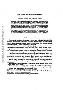
Figure 1:
2
The basic conception of a particle machine
Particle machines
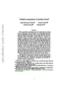
Figure 1 shows the general arrangement of a PM. Particles are injected at one end of the one-dimensional CA, and these particles move through the medium provided by the cells. When two or more particles collide, new particles may be created, existing particles may be annihilated, or no interaction may occur, depending on the types of particles involved in the collision. The state of cell i of a 1-d CA at time t + 1 is determined by the states of cells in the neighborhood of cell i at time t, the neighborhood being de ned to be those cells at a distance, or radius, r or less of cell i. Thus, the neighborhood of a CA with radius r contains k = 2r + 1 cells and includes cell i itself. We think of a cell's n-bit state vector as a binary occupancy vector, each bit representing the presence or absence of one of n particle types (the same idea is used in lattice gasses; see, for example, [2]). The operation of the CA is determined by a rule, called the update rule, which maps states of the cells in the neighborhood of cell i at time t to the state of cell i at time t + 1. Figure 2 illustrates some typical collisions when binary addition is implemented by particle collisions. This particular method of addition will be one of two described later when we develop arithmetic algorithms. The basic idea is that each addend is represented by a stream of particles containing one particle for each bit in the addend, one stream moving left and the other moving right. The two addend streams collide with a ripple-carry adder particle where the addition operation takes place. The ripple-carry particle keeps track of the current value of the carry between collisions of subsequent addend-bit particles as the streams collide least-signi cant-bit rst. As each collision occurs, a new rightmoving result-bit particle is created and the two addend particles are annihilated. Finally, a trailing \reset" particle moving right resets the ripple-carry to zero and creates an additional result-bit particle moving right. We need to be careful to avoid confusion between the bits of the arith3
=
0
=
+0
1
0
1
+0
1
1
1
1
0 =
0
=
1
+1
0
+1
1 0
0 =
0
+1
=
+1
0
0
= 0
+1
+0
Figure 2:
1
0
0
0
An example illustrating some typical particle collisions, and one way to perform addition in a particle machine. What is shown is actually the calculation 01 + 11 = 100, implemented by having the two operands, one moving left and the other moving right, collide at a stationary \ripple-carry" particle. When the leading, least-signi cant bits collide, ingoing from row 2 to 3, the ripple-carry particle changes its identity so that encodes a carry bit of 1, and a rightmoving sum particle representing a bit of 0 is created. The nal answer emerges as the rightmoving stream 100, and the ripple-carry particle is reset by the \equals" particle to encode a carry of 0. The bits of the two addends are annihilated when the sum and carry bits are formed. Notice that the particles are originally separated by empty cells, and that all operations can be e�ected by a CA with a neighborhood size of 3 (a radius 4 of 1).
metic operation and the bits in the state vector. The ripple-carry adder is represented by two particle types, the bits of the rightmoving addend and the rightmoving result are represented by two more particle types, the leftmoving addend bits are represented by another two types, and the reset particle is represented by one additional type. Thus, the operations shown in Fig. 2 use seven bits of the state vector. We'll denote by Ci the Boolean state vector variable for cell i. The individual bits in the state vector will be denoted by bracket notation: for instance, the state vector bit corresponding to a rightmoving zero particle in cell i is denoted Ci [0R]. The seven Boolean variables representing the seven particles are: Ci [0R] rightmoving zero Ci [0L ] leftmoving zero Ci [1R] rightmoving one Ci [1L] leftmoving one Ci [+0] ripple-carry adder w= zero carry
Ci [+1] Ci [=R ]
ripple-carry adder w= one carry rightmoving adder reset
All the particle interactions and transformations shown in the example can be e�ected in a CA with radius one; that is, using only the states of cells i 0 1, i, and i + 1 to update the state of cell i. A typical next-state rule (as illustrated in the rst collision in Fig. 2) therefore looks like Ci [0R](t+1)
( (Ci01[1R] ^ Ci [+0] ^ Ci+1[1L] )(t)
(1)
which says simply that if the colliding addends are 1 and 1, and the carry is 0, then the result bit is a rightmoving 0. Notice that using two state-vector bits to represent one data bit allows us to encode the situation when the particular data bit is simply not present. (Theoretically, it also gives us the opportunity to encode the situation when it is both 0 and 1 simultaneously, although the rules are usually such that this never occurs.) It can be very useful to know a data bit isn't present.
5
C i [+ 0 ] C i-1 [1 R ]
C i+1 [1 L ]
S R out
C i [0 R ]
Figure 3:
The logic fragment of an implementation of the rule in Eq. 1. The
conditions create a rightmoving 0.
3
VLSI size and performance estimate
We base our estimate of VLSI size and performance on a straightforward realization of the rule set as suggested by Fig. 3. In that gure, the rule in Eq. 1 is implemented directly in random logic feeding the inputs to an S-R ip- op that stores one bit of a cell's state vector. This makes it easy to map the rules into logic generally; each rule that creates or destroys a particle sets or resets its corresponding bit. Figure 4 shows the general logic fanning into a state bit. In a practical VLSI implementation the rules would probably be combined and realized in a PLA. The following area estimate assumes this is done. If PMs prove practically useful, it may be worth investing considerable e�ort in optimizing the layout of a PM for a rule set that is su�ciently powerful to implement a wide variety of computations. After all, this design need be done only once, and the resulting chip would be useful in many applications. As with memory cells, only a single cell needs to be designed, which can then be replicated. The chips themselves can be concatenated to form very long | and hence highly parallel | machines. Our layout of a row of cells is shown in Fig. 5. Here each cell has p bits in its state vector, thus supporting p particle types, and contains a logic block, a bank of ip- ops, and wiring connecting logic inputs and outputs to ip- op inputs and outputs. Our estimate of the area required for these 6
values from neighborhood cells
S R out
Figure 4:
flip-flop storing one bit of one cell
A possible layout plan for a PM.
state
PLA
state
PLA
PLA
state
Figure 5:
PLA
state
The general layout of cells in the CA for a PM. The bits in the
state vector are shown as shaded registers. Each such register supplies data to the update logic for its own cell, and those of its nearest neighbor cells. Connections to right neighbors are shown as dashed lines.
elements uses a rough approximation to the space required to route a single signal wire in modern VLSI [9]: about � = 6�, where � = 0:2�. Thus, a wiring channel containing n wires we estimate to be n6� across. We allow four times as much space per signal wire for PLA signal wires, or = 24� per PLA wire. As laid out in Fig. 5, a cell requires vertical space for two wiring channels. In addition, we must t in the larger of either a bank of p ip- ops or the vertical span of the PLA. Since we assume a simple layout, the PLA is the larger structure and we ignore the ip- ops. The PLA contains p input wires, p=3 from the cell's own ip- ops and p=3 each from the two neighbor cells, and p output wires, giving 2p total PLA wires, counting vertically. The total height of a cell is then (2=3)p� + 2p . 7
Horizontally, a cell must accommodate the PLA, two wiring channels, and the ip- ops. The PLA requires roughly as many wires as minterms. Estimating an average of four minterms per output wire, we get 4p horizontal PLA wires. The width of the ip- ops is about 10 PLA wires. A cell's width is then (2=3)p� + 4p + 10 . Let's establish the number of particles required, p, for a general PM. Consider a single track of data. In general for a single track we need data bits that travel in either direction or remain stationary. This requires six particles: 0 and 1 moving left, 0 and 1 moving right, and stationary 0 and 1. Three data tracks su�ce for all applications we have tried. For each data track we assume about six operator particles are needed. This gives us p = 36 total operator and data particles. Using the above area estimates and given a chip 1 centimeter on a side, we nd there is room for about 300 cells on a single chip for a PM supporting 36 particles. Now let's estimate the potential parallel performance. Using the multiplication scheme shown later in Fig. 8 we need about 2n cells to hold a single n-bit operand moving either left or right. The processor particles need 2n cells. This gives 6n total cells between the beginning of one multiply and the beginning of the next multiply. Supposing we have 16-bit operands, this means we can t three 16-bit multiplies operating concurrently on a single chip. The cell logic is very simple, so a conservative estimate of clock speed is 100 Mhz. A multiply completes in 2n ticks. This gives us about 3 million 16-bit integer multiplies per second per chip. Using logic optimization and other layout and performance re nements in the chip design, we might expect to get a factor of 5 to 10 improvement over this estimate.
4 4.1
Compatible collision rules Collision rules
A set of rules in a PM is a relation between preconditions that determine the rule's applicability to collisions and e�ects that give the outcome of collisions. The domain is a set of pairs of the form (PD ; AD ), where PD is a set of particles that must be present in the neighborhood in order for the rule to apply, and AD is a set of particles that must be absent. We refer to particles in AD as particle negations, and we consider particle negations to collide, even though the actual particles are not present. The range is a set of pairs (PR ; AR), where the sets PR and AR give the particles that are created and destroyed, respectively. 8
4.2
Compatibility
When particles collide, two or more collision rules may apply simultaneously to determine the results. For our purposes the e�ects of these rules should not con ict; that is, one such rule should not destroy any particle created by another. If this condition is satis ed, the results of the collision depend only on the colliding particles, not on the order of rule application. We call a rule set of a PM compatible with respect to a set of inputs (or simply compatible) if every collision that occurs is resolved without con icts. We use the term input to include the initial state of the PM's medium, and all particles subsequently injected. Given a PM, we want to be able to determine whether or not its rule set is compatible. The general problem of determining compatibility turns out to be undecidable. However, as we will see, if the PM designer provides certain additional information about the particles, the problem is solvable in time polynomial in the number of particles and rules. 4.2.1
Rule compatibility is undecidable
Theorem 1 The rule compatibility problem is undecidable.
A straightforward reduction from the halting problem. Given a Turing machine M with an initial con guration of its tape, we transform M into a PM, and M 's tape into this PM's input, in such a way that M halts if and only if the PM's rule set is not compatible. Let S , 0, � , and h denote M 's set of states, tape alphabet, transition function, and halt state, respectively. We begin constructing the PM P from M as follows. For each symbol x 2 0, introduce a new stationary particle xp . The tape of the Turing machine then maps directly into the medium of the PM; in particular, the initial con guration of M 's tape corresponds to the initial state of P 's medium. We simulate the transition function � with particles and collision rules. For each state s 2 S , create a stationary particle, sN . This particle is designed to perform the function of M 's tape head. Assume that the transition function is de ned as � : S 2 0 ! S 2 0 [fL; Rg), where L and R are special symbols that indicate left and right movement of the tape head. For all states s and tape symbols x such that � (s; x) is de ned: Proof:
�
If � (s; x) = (t; y ), introduce a rule that transforms the stationary state particle sN to the stationary state particle tN , and transforms the 9
symbol particle xp into the symbol particle yp . This rule simulates M 's changing state and writing a symbol on its tape. � If � (s; x) = (t; L), introduce rules that move the state particle
sN one
cell to the left and transforms sN into tN . These rules simulate M's changing state and moving its tape head to the left.
� If � (s; x) = (t; R), introduce analogous rules to simulate tape head
movement to the right.
To complete the construction, add the stationary particle corresponding to M 's initial state to the cell corresponding to M 's initial head position. The above rules must be compatible, because the medium behaves exactly like M 's tape and the rules operate according to M 's transition function. Finally, choose an arbitrary particle xp and introduce two con icting rules. One rule transforms the particle representing the halt state of M into xp ; the other rule transforms it into xp 's negation. The complete set of rules is compatible if and only if M never halts. 2 4.2.2
Additional information makes compatibility decidable
Although deciding rule compatibility from only the rule set and the input is not possible in general, all is not lost. If the PM designer provides complete information about which pairs of particles can collide, we can determine compatibility with a simple polynomial-time algorithm. The PM designer usually has a good idea of which particles can collide and which cannot, even though computing this information is in general an undecidable problem. For example, a binary arithmetic algorithm most likely uses two particles representing a 0 and a 1 that never coexist in the same cell. The information which the PM designer should provide is an exhaustive list L of pairs of the form (�; ), where � and are particles or negations of particles, and � and can collide. We assume that the designer is willing to guarantee the correctness and completeness of this information, so that if the pair (�; ) is not in the list, then � and can never collide. An easy way to check for rule compatibility is to ensure that each pair of rules in the rule set satis es the following condition: if the rules apply to any collision simultaneously, then the e�ects of the rules do not con ict. The rule e�ects (P1 ; A1 ) and (P2 ; A2) con ict if and only if one rule destroys a particle created by the other; that is, if P1 \ A2 6= ; or P2 \ A1 6= ;. Two rules 10
processor particle addend 1
addend 2
Figure 6: The particle con guration for adding by having the addends collide bit by bit at a single processor particle. with preconditions (P^1; A^1) and (P^2 ; A^2) can be applicable simultaneously only if the following conditions hold: � The rules do not con ict in their preconditions, that is, P^1 \ A^2 = ; and P^2 \ A^1 = ;. � The combined preconditions of the rules contain only pairs (�; ) that can collide; that is, � 2 P^1 [ A^1 and 2 P^2 [ A^2 only if (�; ) 2 L.
It is easy to verify that these conditions can be checked in time polynomial in the number of particles and rules. 5
Linear-time arithmetic
We will conclude this paper with a description of a linear-time PM implementation of Leighton's division algorithm [4]. Before we discuss division, however, we brie y review the implementations of addition and multiplication given in [6, 7]. Note that in all of these implementations, we can consider velocities as relative to an arbitrary frame of reference. We can always change the frame of reference by appropriate changes in the update rules. Figure 6 shows in diagrammatical form the scheme already described in detail in Fig. 2. Figure 7 shows an alternate way to add, in which the addends are stationary, and a ripple-carry particle travels through them, taking with it the bit representing the carry. We can use either scheme to add, simply by injecting the appropriate stream of particles. The choice will depend on the form in which the addends happen to be available in any particular circumstance, and on the form desired for the sum. Note also that negation can be performed easily by sending a particle through a number to complement its bits, and then adding one | assuming we use two's-complement arithmetic. 11
processor particle addend 1 addend 2
Figure 7:
An alternate addition scheme, in which a processor travels through
the addends.
processor particles right multiplicand
left multiplicand
Figure 8:
Multiplication scheme, based on a systolic array.
The processor
particles are stationary and the data particles collide. Product bits are stored in the identity of the processor particles, and carry bits are stored in the identity of the data particles, and thereby transported to neighbor bits.
Figure 7 also illustrates the use of \tracks". In this case two di�erent kinds of particles are used to store data at the same cell position, at the cost of enlarging the particle set. This turns out to be a very useful idea for implementing multiply-accumulators for FIR ltering, and feedback for IIR ltering [7]. The idea is used in the next section for implementing division. Figure 8 shows the particle arrangement for xed-point multiplication. This mirrors the well known systolic array for the same purpose, but of course the structure is \soft" in the sense that it represents only the input stream of the PM which accomplishes the operation. The reader is referred to [6, 7] for more detailed descriptions and a discussion of nested operations and digital ltering. 6
Linear-time division
Although division is much more complicated than the other elementary arithmetic operations, a linear-time, arbitrary-precision algorithm is possible using the particle model. The algorithm we present here, based on Newtonian iteration and described by Leighton [4]1 , calculates the reciprocal of a number x. We assume for simplicity that x is scaled so that 1
The algorithm described here is actually slightly di�erent in some details, but it is not hard to verify its complexity and correctness.
12
path of y 0’s bits
SL SR 0 1 1 1 0 0 0 0 0 0 0 0 0
bits of y 0
1 1 0 0 0 0 0 0 0 0 0 0 0
bits of x 0
path of x 0’s bits
Figure 9: Initial con guration for division.
1 2
�
1. For an arbitrary division problem, we rescale the divisor by shifting its binary point left or right, calculate its reciprocal, multiply by the dividend, and nally scale the result back. Since each of these steps takes only linear time, the entire division uses only linear time. The algorithm works as follows. Let N denote the number of bits desired in the reciprocal. For simplicity, assume N is a power of 2. Let xi represent the i-th approximation of the reciprocal and yi the divisor, both rounded down to 2i+1 + 4 places. Beginning with x0 = 1.1 in binary, the method iterates using xi+1 = xi (2 0 yi xi ), for 0 � i < lg N . At the end of the i-th i +1 iteration, the error is less than 202 . The particle implementation of this algorithm carefully coordinates stationary and moving particles to create a loop. The i-th iteration of the loop performs linear-time, xed-point additions and multiplications using 2i+1 + 4 bits of precision. M arker particles delimit the input number and indicate the bit positions that de ne the successive precisions required by the algorithm. Figure 9 illustrates this setup, giving the initial template for calculating the reciprocal of the number 7 to 8 bits of precision, that is, with error less 1 . The outer markers enclose the binary numbers y0 = 0:111, which than 256 is 7 rescaled to t the algorithm, and x0 = 1.1, the rst approximation to the reciprocal. Additional markers are at bit places 6, 8, and 12 after the binary point, indicating that three iterations are required, at precisions of 6, 8, and 12 bits. Two consecutive markers terminate the number. The only moving particles in Fig. 9 are sender particles, denoted by S L and SR, whose job is to travel through the medium and send data bits to the left and right to begin an iteration of the loop. (The S L and S R particles are created by a chain reaction of previous collisions which will not x