GENERAL-PURPOSE REDUCED-REFERENCE IMAGE QUALITY ASSESSMENT BASED ON PERCEPTUALLY AND STATISTICALLY MOTIVATED IMAGE REPRESENTATION Qiang Li and Zhou Wang Department of Electrical Engineering, The University of Texas at Arlington, Arlington TX, USA Department of Electrical and Computer Engineering, University of Waterloo, Waterloo ON, Canada Email:
[email protected];
[email protected] ABSTRACT Divisive normalization has been recognized as a successful approach to model the perceptual sensitivity of biological vision. It also provides a useful image representation that is well-matched to the statistical properties of natural images. Here we propose a reducedreference image quality assessment method in the divisive normalization transform domain, where the quality of an image is evaluated based on a set of reduced-reference features extracted from a divisive normalization representation of the image. The proposed method is general-purpose, in the sense that no assumption is made about the types of distortions occurred in the image being evaluated. The proposed method is trained and tested using the LIVE database and demonstrates good performance for a wide range of distortions. Index Terms— image quality assessment, perceptual image representation, statistical image modeling, divisive normalization
a local gain-control divisive normalization model has emerged as a powerful method to account for the neuronal responses in biological visual systems [6]. Each coefficient of a linear transform is normalized (divided) by the energy of a cluster of neighboring coefficients. This nonlinear process has been shown to reduce the statistical dependencies of the original linear representation [5] and produce approximately Gaussian marginal distributions [7]. It has also been employed in real world image processing applications, including image compression [8] and image contrast enhancement [3]. The strong perceptual and statistical relevance of divisive normalization representation (as compared to linear decompositions) motivated us to switch from the linear wavelet transform domain (as in [2]) to a divisive normalization transform domain in the development of our RRIQA method. Our experiments show that this results in improved performance for image quality evaluation. 2. METHOD
1. INTRODUCTION Most existing image quality assessment (IQA) methods require full access to the original reference image that is assumed to have perfect quality. Reduced-reference (RR) IQA methods predict the quality degradation of an image with only partial information about the reference image, in the form of a set of RR features [1]. RRIQA methods provide a practically useful and convenient tool for real-time visual information communication and networking systems, where they can be used to track image quality degradations and control the streaming resources on the fly. The major challenge in the design of RRIQA algorithms is to find appropriate RR features that 1) provide an efficient representation of the reference image; 2) are sensitive to various image distortions; and 3) are relevant to the perceptual sensitivity of the human visual system. In previous work, statistical image models have been employed for the purpose of RRIQA. In [2], a generalized Gaussian density function is used to model the marginal statistics of the linear coefficients in a wavelet subband, and the parameters of the fitting model are used as RR features. Although this method achieves notable success, it ignores the strong dependencies between the neighboring wavelet coefficients. In this paper, we propose a new method that is inspired by the recent success of the divisive normalization transform as a perceptually and statistically motivated image representation [3]. It is widely hypothesized in computational vision science that the purpose of early visual sensory processing is to increase the statistical independence between neuronal responses [4]. Linear decompositions can only remove the first-order correlation, but do not reduce the higher order statistical dependencies, such as the variance [5]. Recently,
2.1. Divisive Normalization Computation A convenient approach to compute a divisive normalization representation can be derived from the Gaussian scale mixtures (GSM) model of wavelet coefficients [9]. A length-N random vector Y is a GSM if it can be expressed as the product of two independent com. ponents: Y = zU , where U is a zero-mean Gaussian random vector with covariance CU and z is called a mixing multiplier. Suppose that the mixing density is pz (z), then the density of Y can be written as
Z pY (Y ) =
µ
1 N
[2π] 2 |z 2 CU |1/2
exp −
Y T CU−1 Y 2z 2
¶ pz (z)dz .
(1) This GSM model has shown to be very useful to account for both the marginal and joint statistics of wavelet coefficients [9], where the vector Y is formed by clustering a set of neighboring wavelet coefficients within a subband, or across neighboring subbands. Note that when z is fixed, Y is simply a zero-mean Gaussian vector with covariance z 2 CU . This motivates us to compute a normalized representation by dividing the original wavelet coefficient vector Y by an estimate of z computed from its neighboring coefficients. The coefficient cluster Y is applied as a moving window across a wavelet subband. At each step, only the center coefficient yc of the vector Y is normalized and the new coefficient under the divisive normalization representation becomes yc /ˆ z , where zˆ is the estimate of z. A convenient method to obtain zˆ is by a maximum likelihood estimation [9] given by
Proc. IEEE Inter. Conf. Image Proc., San Diego, CA, USA, Oct. 12-15, 2008
zˆ
=
arg max{log p(Y |z)} z
c IEEE 2008 °
=
arg min{N log z + Y T CU−1 Y /2z 2 }
q
2.3. Reduced-reference Image Quality Assessment
z
Y T CU−1 Y /N .
=
We propose a low data rate RRIQA algorithm, in which only a small set of RR features are extracted from the reference image and are employed in the quality evaluation of the distorted image. First, we apply a wavelet transform to the reference image and compute the divisive normalization transform representation for the coefficients, as described in Section 2.1. We can then draw a histogram of the coefficients at each subband. As being observed in Section 2.2, the probability density function p(x) of the coefficients can be well approximated with a zero-mean Gaussian model:
(2)
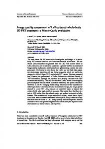
The covariance matrix CU = E[U U T ] is estimated from the entire wavelet subband. 2.2. Image Statistics in Divisive Normalization Representation In Fig. 1, we compare the marginal distributions of an original wavelet subband (computed from a steerable pyramid decomposition [10]) and the same subband after divisive normalization. In Fig. 1(c), the original wavelet coefficient histogram is compared with a Gaussian shape with the same standard deviation. The significant gaps between the two curves indicate that the original wavelet coefficients are highly non-Gaussian. By contrast, the histogram of the coefficients after divisive normalization can be very well fitted with a Gaussian, as shown in Fig. 1(d).
µ
pm (x) = √
Z
0.014
d(pm ||q) =
0.01
0.006
0.002 0
-60
-40
-20
0
(c)
20
40
60
0
(5)
Combining this with the additional RR feature d(pm ||p), we obtain an estimate of the KLD between p(x) and q(x):
0.004
0.01
(4)
pm (x) dx . q(x)
pm (x) log
0.008
0.02
(3)
pm (x) dx p(x)
pm (x) log
Z
(e)
0.012 0.03
,
and use it as an additional RR feature. This is computed for each subband independently, resulting in 2 parameters (σ and d(pm ||p)) for each subband. In order to evaluate the quality of a distorted image, we apply the same divisive normalization transform and obtain the histogram of the transform coefficients at each subband. We can then estimate the KLD between the probability density function q(x) of the coefficients computed from the distorted image and the model pm (x) estimated from the reference image:
(b)
(a)
which requires only one parameter σ to describe. Furthermore, to account for the variations between the model and the true distribution, we compute the Kullback-Leibler distance (KLD) [11] between pm (x) and p(x) as d(pm ||p) =
0.04
1 x2 exp − 2 2σ 2πσ
Z -8
-4
0
4
8
ˆ d(p||q) = d(pm ||q) − d(pm ||p) =
(d)
pm (x) log
p(x) dx . q(x)
(6)
Fig. 1. (a) original wavelet coefficients; (b) normalized coefficients; (c) histogram of original coefficients (solid curve) and a Gaussian curve with the same variance (dashed curve); (d) histogram of normalized coefficients (solid) and a Gaussian fitting (dashed).
Another measure that we found useful for quality evaluation is the difference between the standard deviations of the coefficients computed from the original and distorted images, respectively:
In Fig. 2, we compare the conditional histograms of the coefficients extracted from two neighboring subbands (a parent band and a child band). It can be observed in Fig. 2(a) that in the original wavelet representation, the variance of a child coefficient is highly dependent on the magnitude of its parent coefficient. By contrast, in the divisive normalization representation, the histograms of the child coefficients make little difference when conditioned on the magnitudes of the parent coefficients, as can be seen in Fig. 2(b). This clearly demonstrates that the divisive normalization process reduces the second-order dependencies between the transform coefficients. Figure 3 demonstrates how image distortions change the statistics of the coefficients in the divisive normalization transform domain. It is observed that the original near-Gaussian distribution of these coefficients is sensitive to different types of image distortions, but the way it changes varies with the distortion type. Proper quantification of these changes is the key in the development of our RRIQA algorithm.
Note that this does not increase the number of RR features because σ is already acquired when fitting the Gaussian model of Eq. (3). We define the distortion measure at a subband as a linear combination of ˆ d(p||q) and dσ in the logarithmic domain:
dσ = |σ − σd | .
(7)
¡
¢
α ˆ ˆ Dband = α log(d(p||q)) + β log(dσ ) = log (d(p||q)) (dσ )β , (8) where α and β and weighting parameters. In practice, to avoid the ˆ instability when d(p||q) or dσ is close to zero, we compute
µ Dband = log
α ˆ (d(p||q)) (dσ )β 1+ D0
¶ ,
(9)
where D0 is a positive constant. Finally, the overall distortion is computed as the sum of the distortion measures of all subbands. This distortion measure is always non-negative, and is zero when the original and distorted images are exactly the same. 2
histo (C | P )
Child (C)
histo (C | P ) Child (C)
Parent (P) Parent (P)
-40
-20
0
20
40 -40
-20
0
20
40
-8
(a)
-4
4
0
8
-8
-4
0
4
8
(b)
Fig. 2. Conditional histograms between a parent and a child coefficients extracted from the original wavelet representation (a) and the corresponding divisive normalization representation (b). 0.04
0.04
0.03
0.03
0.02
0.02
0.01
0.01
0 -20
0 -10
0
10
20
-20
-10
0
10
20
(b)
(a) 0.35
0.04
0.3 0.25
0.03
0.2 0.02
0.15 0.1
0.01 0.05 0 -20
-10
0
10
0 -20
20
(c)
-10
0
10
20
(d)
Fig. 3. Histograms of divisive normalization transform coefficients under different image distortions. (a) original “Lena” image; (b) Gaussian noise contaminated image; (c) Gaussain blurred image; (d) JPEG compressed image. Solid curves: histograms of normalized coefficients. Dashed curves: the Gaussian model fitted to the histogram of the original image. Significant departures from the Gaussian model is observed in the distorted images (b), (c) and (d).
different distortion levels. The distortion types include JPEG compression (2 sets), JPEG2000 compression (2 sets), white noise contamination (1 set), Gaussian blur (1 set), and fast fading channel distortion of JPEG2000 compressed bitstream (1 set). There is also a cross-comparison set that mixes images from all distortion types, thus help align the subject scores across different datasets (the alignment is rather crude, and therefore the cross-comparison and all-data tests should only be regarded as useful references). Three methods are used to evaluate how well the objective scores predict the subjective scores: 1) Correlation coefficient between the subjective/objecitve scores after a nonlinear mapping is computed to evaluate prediction accuracy; 2) Spearman rank-order correlation coefficient (ROCC) is calculated to evaluate prediction monotonic-
3. IMPLEMENTATION AND VALIDATION To implement the proposed algorithm, we decompose the image using a steerable pyramid [10] with 3 scales and 4 orientations. For each subband, we apply divisive normalization using 13 neighboring coefficients, including 9 from the same subband, 1 from the parent band, and 3 from the same spatial location in the other orientation bands at the same scale. Two RR features are used for each subband (as described in Section 2.3), resulting in a total of 24 RR features for a reference image. We use the LIVE database [12] to test the proposed algorithm. The database contains seven datasets of 982 subject-rated images created from 29 original images with five types of distortions at 3
Dataset Mean ROCC Std of ROCC
Table 1. JP2(1) 0.9516 1.58e-4
Cross validation using the LIVE database. JP2(2) JPG(1) JPG(1) WN 0.9629 0.8224 0.8976 0.9553 1.21e-4 5.45e-4 1.18e-3 7.30e-4
Std: standard deviation. GBlur FF Cross 0.9590 0.9450 0.8797 5.16e-4 5.69e-4 2.74e-3
Table 2. Performance comparison of IQA methods using the LIVE database JP2(1) JP2(2) JPG(1) JPG(1) WN GBlur FF Cross Correlation Coefficient (prediction accuracy) Proposed 0.9527 0.9685 0.8282 0.9592 0.9644 0.9567 0.9464 0.8921 Wang et al. [2] 0.9353 0.9490 0.8452 0.9695 0.8889 0.8872 0.9175 0.7300 PSNR 0.9337 0.8948 0.9015 0.9136 0.9866 0.7742 0.8811 0.8487 Rank-Order Correlation Coefficient (prediction monotonicity) Proposed 0.9518 0.9629 0.8222 0.8980 0.9554 0.9591 0.9451 0.8786 Wang et al. [2] 0.9298 0.9470 0.8332 0.8908 0.8639 0.9145 0.9162 0.7174 PSNR 0.9231 0.8816 0.8907 0.8077 0.9855 0.7729 0.8785 0.8562 Outlier Ratio (prediction consistency) Proposed 0.0115 0.0122 0.1034 0.0341 0.0000 0.0069 0.0207 0.5600 Wang et al. [2] 0.0690 0.0366 0.1839 0.0341 0.1793 0.1172 0.0621 0.8000 PSNR 0.0805 0.0976 0.092 0.1818 0.0000 0.2069 0.1517 0.7000 Dataset
ity; 3) Outlier ratio is used to evaluate prediction consistency, which is defined as the percentage of predictions outside the range of ±2 standard deviations between subjective scores. Before the proposed algorithm is applied, three model parameters, α, β and D0 , need to be learned from the data. To verify that these parameters are not overtrained, a cross validation method is employed. First, we randomly select 21 out of the 29 original images. We then use all the images created from these 21 images as the training set and use a numerical optimization method to find the best set of parameters. The images created from the remaining 8 original images are used for testing. This process is repeated 50 times, with random partitions of the training and testing sets. We then look at the distribution of the test results, part of which are shown in Table 1. It can be observed that the variations of the ROCC values are small throughout all the test sets. This implies strong robustness and generalization capability of the learned model parameters. To the best of our knowledge, the only other RRIQA algorithm that is general-purpose (as opposed to distortion- or applicationspecific) and has a comparably small RR data rate is the one proposed in [2], which is included in our algorithm comparison. In addition, we also include peak signal-to-noise-ratio (PSNR), which is still the most widely used full-reference IQA measure. Although such comparison is highly unfair to the proposed method and the method in [2] (PSNR requires full access to the original image, as opposed to the 24 scalar features in the proposed method), it provides a useful indication of their relative performance. The comparison results are shown in Table 2. It can be seen that the proposed method produces the best performance in most cases, and the improvement is significant in many cases.
All data 0.9278 1.22e-4
All data 0.9162 0.8226 0.8709 0.9279 0.8437 0.8755 0.1079 0.2311 0.2373
5. REFERENCES [1] Z. Wang and A. C. Bovik, Modern Image Quality Assessment. Morgan & Claypool Publishers, Mar. 2006. [2] Z. Wang, G. Wu, H. R. Sheikh, E. P. Simoncelli, E.-H. Yang, and A. C. Bovik, “Quality-aware images,” IEEE Trans. Image Processing, vol. 15, no. 6, pp. 1680–1689, 2006. [3] S. Lyu and E. P. Simoncelli, “Statistically and perceptually motivated nonlinear image representation,” Proc. SPIE Conf. on Human Vision and Electronic Imaging XII, Jan. 2007. [4] E. P. Simoncelli and B. A. Olshausen., “Natural image statistics and neural representation,” Annual Review of Neuroscience, vol. 24, pp. 1193–1216, May 2001. [5] O. Schwartz and E. P. Simoncelli., “Natural signal statistics and sensory gain control,” Nature neuroscience, vol. 4, pp. 819– 825, Aug. 2001. [6] D. J. Heeger, “Normalization of cell responses in cat striate cortex,” Visual Neural Science, vol. 9, pp. 181–198, 1992. [7] D. L. Ruderman, “The statistics of natural images,” Network: Computation in Neural Systems, vol. 5, pp. 517–548, 1996. [8] J. Malo, I. Epifanio, R. Navarro, and E. P. Simoncelli, “Nonlinear image representation for efficient perceptual coding,” IEEE Trans. Image Processing, vol. 15, pp. 68–80, Jan. 2006. [9] M. J. Wainwright and E. P. Simoncelli, “Scale mixtures of gaussians and the statistics of natural images,” Adv. Neural Information Processing Systems, vol. 12, 1999. [10] E. P. Simoncelli, W. T. Freeman, E. H. Adelson, and D. J. Heeger, “Shiftable multi-scale transforms,” IEEE Trans. Information Theory, Special Issue on Wavelets, vol. 38, pp. 587– 607, Mar. 1992.
4. CONCLUSION We proposed an RRIQA algorithm using statistical features extracted from a divisive normalization-based image representation. The simultaneous perceptual and statistical relevance of this new representation leads to improved performance for image quality assessment. The proposed algorithm has a relatively low data rate for RR features. Furthermore, it does not make any assumption about the image distortion types, thus has the potential to be used for general-purpose in a wide range of applications.
[11] T. M. Cover and J. A. Thomas, Elements of Information Theory. New York: Wiley-Interscience, 1991. [12] H. R. Sheikh, Z. Wang, A. C. Bovik, and L. K. Cormack, “Image and video quality assessment research at LIVE,” http: //live.ece.utexas.edu/research/quality/.
4