Metodološki zvezki, Vol. 10, No. 2, 2013, 99-119
Generalized blockmodeling of sparse networks Aleš Žiberna1
Abstract The paper starts with an observation that the blockmodeling of relatively sparse binary networks (where we also expect sparse non-null blocks) is problematic. The use of regular equivalence often results in almost all units being classified in the same equivalence class, while using structural equivalence (binary version) only finds very small complete blocks. Two possible ways of blockmodeling such networks within a binary generalized blockmodeling approach are presented. It is also shown that sum of squares (homogeneity) generalized blockmodeling according to structural equivalence is appropriate for this task, although it suffers from “the null block problem”. A solution to this problem is suggested that makes the approach even more suitable. All approaches are also applied to an empirical example. My general suggestion is to use either binary blockmodeling according to structural equivalence with different weights for inconsistencies or sum of squares (homogeneity) blockmodeling with null and constrained complete blocks. The second approach is more appropriate when we want complete blocks to have rows and columns of similar densities and differentiate among complete blocks based on densities. If these aspects are not important the first approach is more appropriate as it does in general produce ‘cleaner’ null blocks.
1 Introduction The generalized blockmodeling of relatively sparse binary networks, more specifically of networks where we expect relatively sparse non-null blocks and not completely empty null blocks, is problematic. Sparse networks are defined as networks where the number of ties is of the same order of magnitude as the number of units or where the average degree is much smaller than the number of units (Batagelj and Mrvar, 2001; Mrvar and Batagelj, 2004). Most larger (at least 100 units or more) networks of current scientific interest (Newman, 2004) are sparse, although (generalized) blockmodeling is mainly applied to smaller networks. However, in this paper I limit the discussion to blockmodeling of sparse networks in cases where we also want to allow for sparse non-null blocks (that have densities 1
Aleš Žiberna, Faculty of Social Sciences, University of Ljubljana, Kardeljeva pl. 5, SI -1000 Ljubljana;
[email protected]
100
Aleš Žiberna
below 0.5). I do not discuss blockmodeling of sparse networks when the blocks that are to be found (are desired in the blockmodeling solution) should be dense (i.e. have a density above 0.5) since classical methods based on structural equivalence work well on such networks and therefore this is not a problem to be solved. Blockmodeling is a method for partitioning network units into clusters and, at the same time, partitioning a set of ties into a block (Doreian, Batagelj, and Ferligoj, 2005, p. 29). There are several approaches to blockmodeling, such as stochastic blockmodeling (Anderson, Wasserman, and Faust, 1992; Holland, Laskey, and Leinhardt, 1983; Snijders and Nowicki, 1997), conventional blockmodeling (e. g. Breiger, Boorman, and Arabie, 1975; Burt, 1976; see Doreian et al., 2005, pp. 25–26 for definition) and generalized blockmodeling (Doreian et al., 2005). The main characteristic of generalized blockmodeling is that the equivalence (generalized equivalence (Doreian, Batagelj, and Ferligoj, 1994)) is defined by set of allowed block types (patterns of ties in blocks) and possibly their positions. Since regular blocks (non-null blocks conforming to regular equivalence) can also be (very) sparse, using regular equivalence (Batagelj, Doreian, and Ferligoj, 1992; White and Reitz, 1983; Žiberna, 2009) for the (generalized) blockmodeling of such networks seems reasonable. However, several studies have shown that blockmodeling according to regular equivalence is very sensitive to small changes in the network (Žiberna, 2009; Žnidaršič, Ferligoj, and Doreian, 2012; Žnidaršič, 2012) and is in addition a very weak requirement, often allowing many equally well-fitting partitions (Ferligoj, Doreian, and Batagelj, 2011) or even suggesting that (almost) all units are in the same equivalence class. Yet for binary networks, structural equivalence, which has been shown to be very stable (Žiberna, 2009; Žnidaršič et al., 2012; Žnidaršič, 2012), often cannot be used, especially in sparse networks, because the units that should be equivalent do not necessarily have ties to exactly the same units. The use of structural equivalences in sparse networks is particularly problematic in binary generalized blockmodeling 2 as all blocks with more 0 than 1 ties are classified as null, resulting in only very small complete blocks. This happens with a ‘default’ setting, that is, with the equal weighting of inconsistencies of different block types. The problem can be overcome by choosing suitable weights. Another possibility for blockmodeling sparse networks within binary blockmodeling is to use a density block type (Batagelj, 1997) instead of a complete block type. These possibilities for generalized blockmodeling of sparse networks are explored in the second section. The problem of blockmodeling sparse networks can be overcome by using stochastic equivalence (Holland et al., 1983) which may be said to be the stochastic version of structural equivalence. Two units are stochastically equivalent i f they have the same probabilities of ties to all other units. This means that the
2
Here the terminology from Žiberna (2007a) is used where the generalized blockmodeling for binary networks developed by Doreian, Batagelj and Ferligoj (2005) is called binary (generalized) blockmodeling to distinguish it from generalized blockmodeling for valued networks.
Generalized blockmodeling of sparse networks
101
probabilities of ties within a block are the same for the whole block. However, as these probabilities can also be low this allows for sparse blocks. Something very similar can also be achieved within generalized blockmodeling framework by using sum of squares blockmodeling3 according to structural equivalence (Žiberna, 2007a) on binary networks. When applied to binary networks, this means that sum of squares blockmodeling according to structural equivalence searches for blocks with similar means, which in binary networks comes down to similar densities. It could even be said that it searches for blocks where rows and columns (separately) have similar densities, since blocks gain or lose rows or columns when a unit changes its cluster membership. This makes it similar to stochastic equivalence and also to regular equivalence as it can be said that the attention is shifted from cells to rows and columns (because density does not have a meaning for cells). One problematic characteristic of sum of squares (homogeneity) blockmodeling is that a null block is a special (more restricted) case of a complete block (and in theoretical terms also f-regular and some other blocks) (Žiberna, 2007a), also referred to as “the null block problem” (Žiberna, 2007b, pp. 77–80). In homogeneity (and therefore also sum of squares) blockmodeling, the null block is defined as a block where all tie values are 0, while the complete block as such where all ties values are equal. The consequences of the null block problem appear in two areas. First, a pre-specified blockmodel with null blocks practically cannot be used in sum of squares blockmodeling without also pre-specifying ‘central’ values for non-null (e.g. complete) blocks4. Second, null blocks practically never occur in exploratory analysis since the less restricted versions of the complete blocks are a better fit. This also means that the approach does not optimize towards null blocks because a very sparse block does fit relatively well to a complete block with a very small mean (density in binary networks). In the third section, a solution to this problem is proposed. The main purpose of this paper is to explore ways to perform generalized blockmodeling of relatively sparse binary networks. In the second and third sections, possible approaches to generalized blockmodeling of sparse networks are identified. In the fourth section, these approaches are applied to an empirical example. In the conclusion (the last section), the main points of the paper are summarized and suggestions are given to researchers wishing to use generalized blockmodeling on sparse networks. My general suggestion is to use either binary blockmodeling acc ording to structural equivalence with different weights for inconsistencies in null and complete blocks or sum of squares (homogeneity) blockmodeling with null and constrained complete blocks. The second approach is more appropriate when we want complete blocks to have rows and columns of similar densities and to differentiate among complete blocks based on densities. On the other hand, if these 3
A subtype of homogeneity generalized blockmodeling. This is undesirable as it would diminish most of the advantages of homogeneity blockmodeling. 4
Aleš Žiberna
102
aspects are not important the first approach is more appropriate since it generally produces ‘cleaner’ null blocks.
2 Regular equivalence and partitioning sparse networks
other
options
for
Regular equivalence was first introduced by White and Reitz (1983), by building upon the work of Sailer (1978). Two (groups of) approaches exist for finding groups of regularly equivalent units. The first is to use some version of the REGE algorithm (Borgatti and Everett, 1993; White, 2013) initially developed by White and Reitz based on their 1983 paper, while the other is based on finding regular blocks using local optimization (Batagelj et al., 1992). More details of both approaches for binary and valued networks and a comparison of these two approaches can be found in Žiberna (2008). However, while regular equivalence has been quite extensively studied in the literature in the previously mentioned articles and numerous others (e.g. Borgatti and Everett, 1989; Everett and Borgatti, 1994), it has never achieved widespread use in practice. This is not surprising given that several authors have noticed that finding reasonable groups of regularly equivalent units is problematic. REGE and its variants in the ‘global’ version are unable to find regular equivalence classes in symmetric networks, although there have been some attempts to circumvent this (Doreian, 1987, 1988), while using optimization approaches often leads to many equally well-fitting partitions or unsatisfying partitions (Doreian, Batagelj, and Ferligoj, 2004; Ferligoj et al., 2011). It has also been shown that regular equivalence is very sensitive to small changes in the network (Žiberna, 2009; Žnidaršič et al., 2012; Žnidaršič, 2012). In addition, authors have questioned if regular equivalence is really useful as a concept. Boyd and Jonas (2001) say that it is rarely present in the data and that if their results are confirmed by other authors on other datasets, then “regular equivalence as a default model of social interaction must be abandoned”. Boyd (2002) further says that “Regular equivalence is very beautiful mathematically (see Boyd, 1991), but it is fundamentally flawed sociologically”, while also noticing that it is rarely present in the data. While it may be questionable whether regular equivalence should be used, there is definitely a need for a concept and a method that supports finding blocks that are neither null nor complete in sparse networks. These blocks should also preferably have rows and columns (separately) of similar densities, which would indicate that such rows/columns really are similar and therefore should be in the same blocks. As mentioned in the introduction, binary (generalized) blockmodeling according to structural equivalence (without weighting) or regular equivalence is not appropriate. Using regular equivalence on sparse networks often leads to almost all units being in the same equivalence class, while the remaining classes are usually singletons. The use of structural equivalence on such networks usually leads to
Generalized blockmodeling of sparse networks
103
only very small complete blocks and relatively large and only slightly ‘belowaverage’ dense null blocks. However, there are two possible ways this can be done using binary generalized blockmodeling. The most obvious one is through use of the density block type (Batagelj, 1997) instead of a complete or regular block type. The density block type has zero inconsistency if the density of the block is equal to or above γ (the parameter of the density block type), and equal to the number of ‘missing’ ties to achieve this density otherwise (the exact formulas for this and other block types are available in Batagelj (1997) and Doreian, Batagelj and Ferligoj (2005, p. 224), among others). As the inconsistency of the null block is simply the number of ties in the null block, a block will be classified as a density block and not null if its density is larger than ⁄ . However, the downside of this approach is that there is no incentive 5 for density blocks to have a density over γ or that the rows or columns in the blocks would have similar densities. Another possibility is by using structural equivalence with a different weighting of inconsistencies in null and complete blocks. Doreian, Batagelj and Ferligoj (2005, pp. 186–187) discuss the different weighting of null and complete blocks’ inconsistencies and state that the choice of weights “rests on substantive concerns”, although they do not suggest any specific way of setting these weights. Here I present a suggestion that works reasonably well in sparse networks when the aim is to find denser and sparser blocks, but not perfectly null and especially not perfectly complete blocks. If we want blocks with a density greater than d to be classified as complete and those with a density smaller or equal to d as null, the appropriate ) for complete blocks (or 1 – d for weights would be 1 for null blocks and ⁄( null blocks and d for complete blocks, as only the ratio between the weights is important). The advantage of this approach is that, in spite of this weighting, complete blocks have an incentive to be as dense as possible, although there is still no incentive for similarities in the densities of rows or columns. Let us suppose that we want to find blocks characterized by similar densities of rows and columns. An appropriate concept for finding groups that leads to such blocks is stochastic equivalence (Holland et al., 1983). Based on this definition, numerous stochastic blockmodels have been developed (Airoldi, Blei, Fienberg, and Xing, 2008; Ambroise and Matias, 2012; Anderson et al., 1992; Daudin, Picard, and Robin, 2008; Holland et al., 1983; Latouche, Birmelé, and Ambroise, 2012; McDaid, Murphy, Friel, and Hurley, 2013; Nowicki and Snijders, 2001; Snijders and Nowicki, 1997; Zanghi, Ambroise, and Miele, 2008) which are useful for this task. However, they are currently incompatible with generalized blockmodeling. For applications where generalized blockmodeling is preferred, especially if the use of pre-specified blockmodels is desired, I suggest using sum of squares (homogeneity) blockmodeling. More precisely, the complete blocks from this approach can be used to find blocks compatible with stochastic equivalence , 5
Although blocks obviously cannot have incentives, the term is used in this paper to indicate whether or not the inconsistencies of a certain block type are computed in s uch a way that a change towards a certain property decreases the inconsistencies of the block.
Aleš Žiberna
104
that is to find blocks with similar densities of rows and columns. The approach is explained in more detail in the next section where a modification of the approach is also suggested that enables its use in pre-specified blockmodeling.
3 Homogeneity blockmodeling and the null block problem Homogeneity blockmodeling (Žiberna, 2007a) was developed as an approach to the (generalized) blockmodeling of valued networks. The main idea is that blocks should be as homogenous as possible with respect to some property. When using sum of squares blockmodeling, homogeneity is measured by the sum of squared deviations from the mean or pre-specified value. For complete blocks, the cells’ values should be as homogeneous as possible, while for other blocks other properties within blocks should be homogenous. However, generally the value they should equal is not specified. As a result, this value can also be 0. In such cases, in terms of the ideal structure, practically all other block types reduce to the null block type. In terms of the way inconsistencies are computed , a null block can be seen as a restricted complete block where the value which all (off-diagonal) values should be equal to is restricted to 0. If the sum of squares approach is used, the optimal value for a complete block, that is the value from which sum of squares deviations (inconsistency) is the smallest, is the mean (density in the case of binary networks) of all the (off-diagonal) tie values and thus, if at least one value is not zero (and only positive values are present), the null block will have greater inconsistency than the complete block. As a result, null blocks are hardly ever identified and sparse blocks are classified as complete. As such, there are fewer penalties for them not being completely empty. This problem is already identified and was named “the null block problem” in Žiberna (2007b, pp. 77–80) where some solutions that more or less circumvent this problem are suggested. A solution that is suggested here is to restrict all non-null block types so that the value to which the values should be homogeneous is restricted to be larger than or equal to some pre-specified threshold. This means that when computing deviations for the computation of block inconsistencies (see Žiberna (2007a) for how inconsistencies are generally computed for homogeneity blockmodeling), these deviations within non-null blocks are computed from the optimal value if such a value is equal to or larger than the pre-specified value, and from the prespecified value otherwise. The formula for computing inconsistencies for the sum of squares blockmodeling of an off-diagonal complete block is given in Equation 3.1: ̅) ∑ ∑( if ̅ ∑ ∑( {
)
( otherwise
)
Generalized blockmodeling of sparse networks
105
Where: is the computed block inconsistency ̅ is the mean of the block is the row cluster is the column cluster is the value of the tie from unit i to unit j is the pre-specifed value In this way, if only null and complete blocks are used within the sum of squares approach, there are incentives for blocks to either have a mean equal to 0 (or close to 0) or higher than or equal to a pre-specified value. For complete blocks, a reasonable choice for the pre-specified value is twice the mean of the network. In case only null and complete blocks are allowed, the blocks will thereby be classified as complete if the block mean is larger than the mean of the whole network. Based on my experience and testing on several networks, such a selection of the pre-specified value produces very good or at least reasonable results in most networks, although other values can be used if a different ‘threshold’ for classification is desired (e.g. if driven by subject knowledge). However, the results in most cases are not very sensitive to the selection of this pre-specified value (so long as it is not too high) because the inconsistency in the constrained complete blocks can always be computed from a value higher than the threshold (and in most blocks it is). The use of constrained non-null blocks is appropriate whenever null blocks are desired. This is especially important in situations where pre -specified blockmodeling is performed. Of course, this constraint can be used in any non-null blocks, regardless of the type and whether they appear on the diagonal or not. For the diagonal block, the restriction is usually only implemented off the diagonal (if a special version of the diagonal blocks exists for the block type).
4 Example: Application to network of the elite of cancer researchers in France The suggested approach is demonstrated on a network of the elite of cancer researchers in France (Lazega, Jourda, Mounier, and Stofer, 2008). Through interviews, Lazega et al. gathered several networks of researchers, several networks of labs (laboratories) and a two-mode network of researchers’ membership in labs. However, for this demonstration, only the aggregated network of researchers (several relations were merged) is used (employing the same kind of aggregation performed by Lazega et al. (2008)). This aggregate network of researchers measures which researchers each researcher specified as their collaborator/s. The network is presented using the graph in Figure 1 and the matrix in Figure 2. We can see from the figures and network statistics in Table 1 that the network is relatively sparse. While there are some researchers with many ties, most of them
Aleš Žiberna
106
only have a few ties. This is the kind of network where in most cases binary blockmodeling according to either structural or regular equivalence does not produce satisfactory results. The density value is used in several places in this example. A slightly rounded value is used and denoted as d = 0.06.
Figure 1: Graph representation of the network
Figure 2: Matrix representation of the network (researchers are ordered according to the all-degree)
Generalized blockmodeling of sparse networks
107
Table 1: Basic network statistics Statistics Number of units Number of ties Density Average in-degree Centralization all-degree Centralization in-degree Centralization out-degree Centralization betweenness centrality Clustering coefficient Reciprocity
Value 127 986 0.061 7.764 0.167 0.122 0.210 0.099 0.281 0.368
In this example, both binary blockmodeling and sum of squares blockmodeling are applied to this network. For the binary blockmodeling, several approaches are tested: Structural equivalence (null and complete blocks are allowed) with equal weighting of inconsistencies. Structural equivalence where null blocks’ inconsistencies have a weight 1 ) ≈ 0.064, and complete blocks’ inconsistencies are weighted by ⁄( where d = 0.06 is (approximately) the density of the network. Regular equivalence (null, complete and regular blocks are allowed). Equivalence with allowed block types: o null block type o density block type with parameter γ = 2d = 0.12. In addition, two versions of sum of squares blockmodeling are used: Structural equivalence with null and complete blocks allowed (however, null blocks are a special case of complete blocks) – not used in pre-specified designs. Equivalence with allowed block types: o Null block type o Restricted complete block type with the pre-specified restriction p = 2d = 0.12. All approaches discussed are applied to the following two models: A free (no pre-specifications) model A cohesive groups (non-null blocks on the diagonal and null blocks offdiagonal of the image matrix) model An exception is sum of squares blockmodeling according to structural equivalence (with unrestricted complete blocks), which is unsuitable for pre-specified blockmodeling and is therefore not used for the second model. The cohesive groups model was chosen as it is a very restrictive model (each blocks has only one allowed block type). Based on my experience in such cases, even binary blockmodeling according to structural equivalence with equal weights of inconsistencies can produce reasonable results.
Aleš Žiberna
108
4.1 The free model Under the free (no pre-specification) model, binary blockmodeling according to either structural (unweighted inconsistencies) or regular equivalence does not (as expected) produce satisfactory results. For structural equivalence, the most suitable number6 of clusters based on the plot of inconsistencies by the number of clusters (see Figure 3) is 3 (6 and 8 would also be possible candidates). The number of different solutions with the lowest inconsistency is indicated by the size of the points. The partitioned matrix into 2 to 7 clusters is presented in Figure 4. Here we can see that in the 3-cluster partition, two internally densely connected clusters are identified as well as one large cluster with no specific pattern of connections. When the number of clusters is further increased, this large cluster is only slightly reduced (from 110 units in the 3-cluster partition to 102 and 89 units in 7- and 8cluster partitions, respectively). Therefore, binary blockmodeling according to structural equivalence is appropriate for detecting dense blocks which translate to the identification of a few small groups, but it is inappropriate for determining a more general partition of the network.
Figure 3: Inconsistencies by number of clusters for binary blockmodeling according to structural equivalence (unweighted). The point size indicates the number of different solutions with the lowest inconsistency.
Binary blockmodeling according to regular equivalence produced, as expected, even worse results. Regardless of the number of clusters (2 – 8) we obtain one cluster with 117 units (out of 127) that is connected to itself with a perfect (zero inconsistency) regular block. Such a partition is obviously useless (the results are omitted here to save space).
6
The most suitable number is the one after the highest reduction of the inconsistency.
Generalized blockmodeling of sparse networks
109
Figure 4: Matrix partitioned using binary blockmodeling according to structural equivalence
Somewhat better results are obtained with binary blockmodeling when allowing null and density block types, where the density threshold γ was set to
Aleš Žiberna
110
approximately twice the density (0.12) to classify blocks denser than the density of the whole network as density type blocks, and as null otherwise. From the inconsistencies presented in the left half of Figure 5 it is clear that 5-cluster solution is the most appropriate. The matrix partitioned according to this partition is presented in the right half of the same figure.
Figure 5: Results of the binary blockmodeling with null and density blocks. In the left plot the point size indicates the number of different solutions with the lowest inconsistency.
The corresponding block densities are shown in Table 2. The image matrix is indicated in Table 2 with a black background and with numbers being used for density blocks (those with a density above 0.06), and vice versa for null blocks. While this is a usable partition, most density blocks have a density approximately equal to the density threshold γ (0.12). They therefore have a very similar de nsity and are thus not as dense as at least some could be. This is expected because this approach does not give any incentives for blocks to be denser than the density threshold γ of the density blocks. Denser blocks could of course be found by increasing this density threshold, albeit at the expense of more (even not very sparse) blocks being classified as null blocks. This also shows that the approach is very sensitive to the selection of the density threshold γ. Table 2: Block densities (ignoring the diagonal for diagonal blocks) for the binary blockmodeling with null and density blocks, 5-cluster partition. Black background indicates non-null blocks.
1 2 3 4 5
1 0.132 0.119 0.118 0.023 0.008
2 0.121 0.123 0.009 0.009 0.008
3 0.123 0.008 0.121 0.004 0.009
4 0.111 0.021 0.021 0.122 0.009
5 0.021 0.008 0.014 0.009 0.026
Generalized blockmodeling of sparse networks
111
The best approach within binary blockmodeling for partitioning such networks seems to be to use structural equivalence with different weights for null and complete blocks’ inconsistencies. As with the approach using density blocks, we set the weights so that blocks denser than the density of the whole networks are classified as complete and the rest as null. This criterion for the selection of weights (introduced in Section 2) leads to using weight 1 for null blocks’ inconsistencies and 0.064 for complete blocks’ inconsistencies. Based on the inconsistencies by number of clusters presented in the left half of Figure 6, we can see that the 5- or 7-cluster solution is the most appropriate. I chose the 5-cluster solution for simplicity and to allow an easier comparison with the previous solution. The matrix partitioned according to this partition is presented in the right half of the same figure. The corresponding block densities are shown in Table 3. The image matrix is indicated in Table 3 with a black background and with numbers being used for complete blocks, and vice versa for null blocks. This could also be determined solely from the densities as all blocks with a density above 0.06 are classified as complete and the others as null. Compared to the previous solution (with density blocks), here not all non-null7 blocks have practically the same densities. Some have much higher densities, while others are lower due to the fact that the criterion function does not ‘break’ at density of 0.12. However, ‘the costs’ of these differential densities are somewhat larger densities of null blocks and not such a clear distinction between the null and non-null blocks. However, I still prefer this solution as it tells more about the structure of the network (and less about the exploratory method used).
Figure 6: Results of the binary blockmodeling according to structural equivalence with different weights for the null and complete blocks' inconsistencies. In the left plot the point size indicates the square root (due to big differences) of the number of different solutions with the lowest inconsistences.
7
The term “non-null blocks” is used here as it includes all blocks other than null, therefore also both complete and density blocks.
Aleš Žiberna
112
Table 3: Block densities (ignoring the diagonal for diagonal blocks) for binary blockmodeling according to structural equivalence with different weights, 5-cluster partition. Black background indicates non-null blocks.
1 2 3 4 5
1 0.283 0.084 0.144 0.116 0.016
2 0.130 0.255 0.021 0.021 0.014
3 0.182 0.012 0.140 0.012 0.014
4 0.172 0.010 0.015 0.166 0.014
5 0.037 0.016 0.009 0.02 0.027
The same network was also analyzed using sum of squares blockmodeling according to structural equivalence. First the (null and) unconstrained complete blocks were used. Based on the inconsistencies by number of clusters presented in the left half of Figure 7, we can see that the 3-cluster solution is the most appropriate. The matrix partitioned according to this partition is presented in the right half of the same figure. The corresponding block densities are shown in Table 4. The image matrix is not presented because under this approach all blocks are classified as complete (as discussed in Section 3). While this solution nicely discovers the two cohesive groups (one very cohesive, much more than any previously found), it fails to capture the structure evident from the two best solutions obtained using binary blockmodeling (in Figure 5 and Figure 6). Further, the ‘null-like’8 blocks are not as sparse as those in the previously mentioned solutions.
Figure 7: Results of the sum of squares blockmodeling according to structural equivalence. In the left plot the point size indicates the number of different solutions with the lowest inconsistency.
8
As mentioned in Section 3, true null blocks are almost impossible.
Generalized blockmodeling of sparse networks
113
Table 4: Block densities (ignoring the diagonal for diagonal blocks) for sum of squares blockmodeling according to structural equivalence, 3-cluster partition
1 2 3
1 0.628 0.035 0.025
2 0.050 0.230 0.034
3 0.069 0.057 0.032
The final approach I applied to this network is sum of squares blockmodeling with null and constrained complete blocks. The null blocks are constrained so that the value from which the inconsistencies are computed is at least (p in Equation 3.1) 0.12. Based on the inconsistencies by number of clusters presented in the left half of Figure 8, we can see that the 3-cluster solution is the most appropriate. The matrix partitioned according to this partition is presented in the right half of the same figure. The corresponding block densities are shown in Table 5. The image matrix is indicated in this table with a black background and white numbers being used for complete blocks, and vice versa for null blocks.
Figure 8: Results of the sum of squares blockmodeling with null and constrained complete blocks. In the left plot the point size indicates the number of different solutions with the lowest inconsistency. Table 5: Block densities (ignoring the diagonal for diagonal blocks) for the sum of squares blockmodeling with null and constrained complete blocks, 3-cluster partition. Black background indicates non-null blocks.
1 2 3
1 0.628 0.034 0.024
2 0.042 0.184 0.027
3 0.078 0.045 0.025
We can see that the results are very similar to the unrestricted structural equivalence results. The only difference in partitions is that 11 units from the third cluster in the unrestricted structural equivalence partition have moved to the second
114
Aleš Žiberna
cluster. The result in terms of densities is that the destines that were the closest to the mean density have moved further from it, while one that was far away from it has moved closer. An additional benefit is that we automatically obtain the categorization of blocks into null and complete. While this could be done manually in this case, it also makes the use of pre-specified blockmodeling possible. The advantage of both of these two approaches (sum of squares blockmodeling) is that they not only differentiate among null and complete blocks, but also among complete blocks of different densities. The cost of this is, however, less ‘empty’ null blocks.
4.2 The cohesive groups model A similar analysis was performed using the cohesive groups pre -specified model. In order to save space, only the best results are presented here. All approaches except binary blockmodeling according to regular equivalence produced sensible results, although for binary blockmodeling with null and density blocks this is only true when up to 4 clusters were requested. The best results were obtained using binary blockmodeling and sum of squares blockmodeling with null and constrained complete blocks. For these two approaches, 3- or 4-cluster solutions are the most appropriate and are presented in Figure 9. Here we can again notice that sum of squares blockmodeling differentiates based on densities. The consequences of this are that the complete blocks (on the diagonal in this case) usually have significantly different densities and that rows and columns (each separately) inside the complete blocks have similar densities. However, the consequence of this additional optimizational aspect (similar densities of rows and columns within complete blocks) is that there are more ties in the off-diagonal blocks and less in the blocks on the diagonal (where they should be).
5 Software All of the approaches were applied using the development version of the blockmodeling 0.2.2 package (Žiberna, 2013a, 2013b) within the R 3.0.1 software environment for statistical computing and graphics (R Core Team, 2013). The source code used for the results presented in the paper is available as supplementary material (without data).
6 Discussion and conclusion The generalized blockmodeling of relatively sparse networks (where we also expect sparse non-null blocks) is problematic. I identified two ways that classical binary generalized blockmodeling could be used for blockmodeling such networks. The most obvious choice is to use density blocks, although a shortcoming of this approach is that there is no incentive for these density blocks to have densities above the selected threshold. The other approach is to use structural equivalence where different weights are given to inconsistencies in null and complete blocks,
Generalized blockmodeling of sparse networks
115
noting that I suggested how these weights should be computed. The advantage of this second approach is that the incentive remains for complete blocks to be as dense as possible. Another possible approach is to use sum of squares (homogeneity) blockmodeling according to structural equivalence. Two versions of this approach, with restricted and unrestricted complete blocks, are discussed. The advantage of this approach (both versions) is that it searches for complete blocks with similarly dense rows and columns and consequently differentiates complete blocks of different densities; however, the cost of this additional optim ization criterion is that more ties are present in the null blocks.
Figure 9: Matrix partitioned into 3 and 4 clusters according to the cohesive groups prespecified blockmodel by binary blockmodeling according to structural equivalence and by sum of squares blockmodeling with null and restricted complete blocks
All these approaches/versions produce reasonable results when applied to the analyzed network and all other sparse binary networks on which I tested them.
116
Aleš Žiberna
They therefore represent a general way of blockmodeling sparse networks when the aim is to find groups that are connected with relatively weak ties (sparse blocks). It should be noted that structural equivalence with equal weights for null and complete blocks’ inconsistencies can also produce very good results when used with a very stringently pre-specified blockmodel (e.g. a cohesive groups model or any model where only one block type is allowed per position). We have seen that several approaches produce satisfactory results. While the most suitable approach may vary by the type of problem, the desired characteristics of blocks sought and the network analyzed, a general suggestion is to use either binary blockmodeling according to structural equivalence with different weights for inconsistencies in null and complete blocks or sum of squares blockmodeling with null and constrained complete blocks. The second approach i s more appropriate when we want complete blocks to have rows and columns of similar densities and to differentiate complete blocks based on densities. Conversely, if these aspects are not important the first approach 9 is more appropriate because it generally produces ‘cleaner’ null blocks. Of course, this paper has some limitations that represent possibilities for future research. The first one is that the approach was only tested on a limited number of sparse networks and further testing is required. As mentioned above, the suggested approaches are appropriate when the aim is to find groups connected with relatively weak ties (sparse blocks). The second limitation is that it is, however, not clear when such partitions are of substantial interest. Further research is needed to answer this question, although initial results indicate that these approaches are more appropriate for finding a smaller number of larger, more general, groups.
References [1] Airoldi, E. M., Blei, D. M., Fienberg, S. E., and Xing, E. P. (2008): Mixed Membership Stochastic Blockmodels. J. Mach. Learn. Res., 9, 1981–2014. [2] Ambroise, C., and Matias, C. (2012): New consistent and asymptotically normal parameter estimates for random-graph mixture models. Journal of the Royal Statistical Society: Series B (Statistical Methodology), 74(1), 3–35. doi:10.1111/j.1467-9868.2011.01009.x [3] Anderson, C. J., Wasserman, S., and Faust, K. (1992): Building stochastic blockmodels. Social Networks, 14(1–2), 137–161. doi:10.1016/03788733(92)90017-2 [4] Batagelj, V. (1997): Notes on blockmodeling. Social Networks, 19, 143–155. [5] Batagelj, V., Doreian, P., and Ferligoj, A. (1992): An optimizational approach to regular equivalence. Social Networks, 14, 121–135.
9
Binary blockmodeling according to structural equivalence with different weights for inconsistencies in null and complete blocks
Generalized blockmodeling of sparse networks
117
[6] Batagelj, V., and Mrvar, A. (2001): A subquadratic triad census algorithm for large sparse networks with small maximum degree. Social Networks, 23(3), 237–243. doi:10.1016/S0378-8733(01)00035-1 [7] Borgatti, S. P., and Everett, M. G. (1989): The class of all regular equivalences: Algebraic structure and computation. Social Networks, 11(1), 65–88. doi:10.1016/0378-8733(89)90018-X [8] Borgatti, S. P., and Everett, M. G. (1993): Two algorithms for computing regular equivalence. Social Networks, 15(4), 361–376. doi:10.1016/03788733(93)90012-A [9] Boyd, J. P. (2002): Finding and testing regular equivalence. Social Networks, 24(4), 315–331. doi:10.1016/S0378-8733(02)00011-4 [10] Boyd, J. P., and Jonas, K. J. (2001): Are social equivalences ever regular?: Permutation and exact tests. Social Networks, 23(2), 87–123. doi:10.1016/S0378-8733(01)00032-6 [11] Breiger, R., Boorman, S., and Arabie, P. (1975): Algorithm for Clustering Relational Data with Applications to Social Network Analysis and Comparison with Multidimensional-Scaling. Journal of Mathematical Psychology, 12(3), 328–383. doi:10.1016/0022-2496(75)90028-0 [12] Burt, R. (1976): Positions in Networks. Social Forces, 55(1), 93–122. doi:10.2307/2577097 [13] Daudin, J.-J., Picard, F., and Robin, S. (2008): A mixture model for random graphs. Statistics and Computing, 18(2), 173–183. doi:10.1007/s11222-0079046-7 [14] Doreian, P. (1987): Measuring regular equivalence in symmetric structures. Social Networks, 9(2), 89–107. doi:10.1016/0378-8733(87)90008-6 [15] Doreian, P. (1988): Borgatti toppings on Doreian splits: Reflections on regular equivalence. Social Networks, 10(3), 273–285. doi:10.1016/03788733(88)90017-2 [16] Doreian, P., Batagelj, V., and Ferligoj, A. (1994): Partitioning networks based on generalized concepts of equivalence. The Journal of Mathematical Sociology, 19(1), 1–27. doi:10.1080/0022250X.1994.9990133 [17] Doreian, P., Batagelj, V., and Ferligoj, A. (2004): Generalized blockmodeling of two-mode network data. Social Networks, 26, 29–53. doi:10.1016/j.socnet.2004.01.002 [18] Doreian, P., Batagelj, V., and Ferligoj, A. (2005): Generalized Blockmodeling. Cambridge University Press. [19] Everett, M. G., and Borgatti, S. P. (1994): Regular equivalence: General theory. The Journal of Mathematical Sociology, 19(1), 29–52. doi:10.1080/0022250X.1994.9990134 [20] Ferligoj, A., Doreian, P., and Batagelj, V. (2011): Positions and roles. In J. Scott and P. J. Carrington (Eds.): The SAGE handbook of social network analysis, 434–446. Los Angeles: SAGE Publications.
118
Aleš Žiberna
[21] Holland, P. W., Laskey, K. B., and Leinhardt, S. (1983): Stochastic blockmodels: First steps. Social Networks, 5(2), 109–137. doi:10.1016/03788733(83)90021-7 [22] Latouche, P., Birmelé, E., and Ambroise, C. (2012): Variational Bayesian inference and complexity control for stochastic block models. Statistical Modelling, 12(1), 93–115. doi:10.1177/1471082X1001200105 [23] Lazega, E., Jourda, M.-T., Mounier, L., and Stofer, R. (2008): Catching up with big fish in the big pond? Multi-level network analysis through linked design. Social Networks, 30(2), 159–176. doi:10.1016/j.socnet.2008.02.001 [24] McDaid, A. F., Murphy, T. B., Friel, N., and Hurley, N. J. (2013): Improved Bayesian inference for the stochastic block model with application to large networks. Computational Statistics & Data Analysis, 60, 12–31. doi:10.1016/j.csda.2012.10.021 [25] Mrvar, A., and Batagelj, V. (2004): Relinking marriages in genealogies. Metodološki zvezki - Advances in Methodology and Statistics, 1, 407–418. [26] Newman, M. E. J. (2004): Fast algorithm for detecting community structure in networks. Physical Review E, 69(6), 066133. doi:10.1103/PhysRevE.69.066133 [27] Nowicki, K., and Snijders, T. A. B. (2001): Estimation and prediction for stochastic blockstructures. Journal of the American Statistical Association, 96, 1077–1087. [28] R Core Team (2013): R: A Language and Environment for Statistical Computing. Vienna, Austria. Retrieved from http://www.R-project.org/ [29] Sailer, L. D. (1978): Structural equivalence: Meaning and definition, computation and application. Social Networks, 1(1), 73–90. doi:10.1016/03788733(78)90014-X [30] Snijders, T. A. B., and Nowicki, K. (1997): Estimation and prediction for stochastic blockmodels for graphs with latent block structure. Journal of Classification, 14, 75–100. [31] White, D. R. (2013, January 22): REGGE (web page). . Retrieved January 22, 2013, from http://eclectic.ss.uci.edu/~drwhite/REGGE/ [32] White, D. R., and Reitz, K. P. (1983): Graph and Semigroup Homomorphisms on Networks of Relations. Social Networks, 5(2), 193–234. doi:10.1016/03788733(83)90025-4 [33] Zanghi, H., Ambroise, C., and Miele, V. (2008): Fast online graph clustering via Erdős–Rényi mixture. Pattern Recognition, 41(12), 3592–3599. doi:10.1016/j.patcog.2008.06.019 [34] Žiberna, A. (2007a): Generalized blockmodeling of valued networks. Social Networks, 29, 105–126. doi:10.1016/j.socnet.2006.04.002 [35] Žiberna, A. (2007b): Generalized blockmodeling of valued networks (Posplošeno bločno modeliranje omrežij z vrednostmi na povezavah) : doktorska disertacija. University of Ljubljana, Ljubljana.
Generalized blockmodeling of sparse networks
119
[36] Žiberna, A. (2008): Direct and indirect approaches to blockmodeling of valued networks in terms of regular equivalence. Journal of Mathematical Sociology, 32, 57–84. doi:10.1080/00222500701790207 [37] Žiberna, A. (2009): Evaluation of Direct and Indirect Blockmodeling of Regular Equivalence in Valued Networks by Simulations. Metodološki Zvezki, 6(2), 99–134. [38] Žiberna, A. (2013a): blockmodeling: An R package for Generalized and classical blockmodeling of valued networks. Retrieved December 3, 2013, from http://www2.arnes.si/~aziber4/blockmodeling/ [39] Žiberna, A. (2013b): R-Forge: blockmodeling: R Development Page. Retrieved December 3, 2013, from https://r-forge.rproject.org/R/?group_id=203 [40] Žnidaršič, A. (2012): Stability of blockmodeling (Stabilnost bločnega modeliranja) : doktorska disertacija. University of Ljubljana. Retrieved from http://dk.fdv.uni-lj.si/doktorska_dela/pdfs/dr_znidarsic-anja.PDF [41] Žnidaršič, A., Ferligoj, A., and Doreian, P. (2012): Non-response in social networks: The impact of different non-response treatments on the stability of blockmodels. Social Networks, 34(4), 438–450. doi:10.1016/j.socnet.2012.02.002