{justinian.rosca,christian.borss,radu.balan}@scr.siemens.com. ABSTRACT. Sparse constraints on signal decompositions are justified by typical sensor data ...
GENERALIZED SPARSE SIGNAL MIXING MODEL AND APPLICATION TO NOISY BLIND SOURCE SEPARATION Justinian Rosca, Christian Borss, Radu Balan Siemens Corporate Research, 755 College Road East, Princeton, NJ 08540 {justinian.rosca,christian.borss,radu.balan}@scr.siemens.com ABSTRACT Sparse constraints on signal decompositions are justified by typical sensor data used in a variety of signal processing fields such as acoustics, medical imaging, or wireless, but moreover can lead to more effective algorithms. The specific sparseness assumption used in this work is that the maximum number of statistically independent sources active at any time and frequency point in a mixture of signals is small. This is shown to result from an assumption of sparseness of the sources themselves, and allows us to solve the maximum likelihood formulation of the non-instantaneous acoustic mixing source estimation problem. We consider an additive noise mixing model with an arbitrary number of sensors and possibly more sources than sensors, when sources satisfy the sparseness assumption above. The solution obtained is applicable to an arbitrary number of microphones and sources, but works best when the number of sources simultaneously active at any time frequency point is a small fraction of the total number of sources. 1. INTRODUCTION The idea of a sparse signal representation is to transform signal data into a domain where data can be parsimoniously described (for instance by a superposition of a small number of basis) or, more generally, has a small �p -norm (0 ≤ p ≤ 1) [1, 2, 3]. Typical signal transformations are the Fourier, the wavelet transform, or independent component analysis (ICA) transformations adapted to the data [4]. Taking sparseness as a prior assumption about signal models is often justified by the nature of signals (e.g. natural images [5], sounds [6]). More importantly, the assumption can lead to effective algorithms for signal separation. This has been the case in applications ranging from audio source separation to medical and image signal processing [7]. The subject of this paper is twofold. First we discuss the form of our sparsity assumption, then we present its application to blind source separation of noisy real-world audio signals. Our sparsity assumption is given by a constraint on the maximum number of statistically independent sources present in a mixture of signals at any time and frequency point. This is a generalization of the assumption – that time-frequency representations of any two sources do not overlap – used in [8], which introduced a BSS technique for the separation of an arbitrary number of sources from just two mixtures. The key observation in the technique was that each time-frequency (TF) point depended on at most one IN PROCEEDINGS OF ICASSP 2004, MONTREAL CANADA, MAY 2004
source and its associated mixing parameters. This deterministic hypothesis was called W-disjoint orthogonality. In anechoic nonnoisy environments, it is possible to extract the mixing parameters from the ratio of the TF representations of the mixtures. Using the mixing parameters, one can partition the TF representation of the mixtures to produce the original sources. The deterministic signal model was extended to a stochastic signal model in [9], where each time-frequency coefficient was modeled as a product between a continuous random variable and a 0/1 discrete Bernoulli random variable (indicating the “presence” of the source). This way signals can be modeled as independent random variables, and one can derive the maximum likelihood (ML) estimator of the mixing parameters. The approach has good results on real data even for more sources than sensors and has been further analyzed in the literature. However, the sparse nature of the signal estimates implies that their time-domain reconstruction by time-frequency masking will contain artefacts. The problem is alleviated in [10] by combination of masking and ICA. In this paper we deal with a multi-channel (D > 2) extension in the presence of noise by exploring a generalization of the sparsity assumptions from [8, 9, 11]. We further extend the ML estimators derived before. The ML approach considers both mixing parameters and sources, unlike in [12] where the optimization was over mixing parameters only. The rest of the paper is organized as follows. Section 2 presents a statistical motivation of the sparseness assumption, its generalization, and the mixing model. Section 3 shows the derivation of the ML estimator of the mixing parameters and the source signals. Section 4 focuses on the capability of the algorithm under the assumption that either one or only two sources are active at any time frequency point. Experiments use eight sensors and four voice mixtures in the presence of noise and show enhanced intelligibility of speech under the more general sparsity assumption. 2. MIXING MODEL ASSUMPTIONS 2.1. Sparseness and the Generalized W-Disjoint Orthogonality Hypothesis In [12] we called two signals s1 and s2 W-disjoint orthogonal, for a given windowing function W (t), if the supports of the windowed Fourier transforms of s1 and s2 are disjoint, that is: S1 (k, ω)S2 (k, ω) = 0 , ∀k, ω
(1)
This deterministic assumption implies that the signals are in general statistically dependent, which is not the case. Yet, relation
(1) is satisfied in an approximate sense (e.g. in particular by real speech signals [13]). Furthermore, [11] shows that relation (1) can be seen as the limit of a stochastic model introduced in [9]. Here we generalize this model and show that it follows from a sparsness prior. We call L signals s1 , s2 , . . . , sL generalized Wdisjoint orthogonal (or N -term W-disjoint orthogonal) if for every time-frequency point (t, ω), there are L−N indices {jN+1 , . . . , jN } in {1, 2, . . . , L} so that Sjk (t, ω) = 0 , ∀N + 1 ≤ k ≤ L.
(2)
We briefly review the model and signal class from [9]. It states that the time-frequency coefficient S(k, ω) of a (speech) signal s(t) factors as a product of a continuous random variable, say G(k, ω), and a 0/1 Bernoulli V (k, ω):
2.2. Mixing Model Next we introduce a specific additive noise mixing model for noninstantaneous audio signals, where sensor noises are assumed independently distributed and have Gaussian distributions with zero mean and σ2 variance. Consider the measurements of L source signals by a equispaced linear array of D sensors under a far-field assumption where only the direct path is present. In this case, without loss of generality, we can absorb the attenuation and delay parameters of the first mixture x1 (t), into the definition of the sources. Furthermore, for the purposes of this paper we neglect the relative attenuation between sensors. x1 (t)
pS (S) = qp(S) + (1 − q)δ(S)
(4)
with δ, the Dirac distribution. For L independent signals S1 , . . . , SL , the joint p.d.f. is obtained by conditioning with respect to the Bernoulli random variables. To simplify the notation, we assume all G(k, ω) have the same distribution p(·), and all V (k, ω) have the same q. We obtain:
=
L �
=
(qp(S) + (1 − q)δ(S))L �
q k (1 − q)L−k
k �
(5) L �
p(Saj )
1≤a1 ≤a2 ≤···≤ak ≤L j=1
k=0
δ(Saj )
j=k+1
where {a1 , a2 , . . . , aL } = {1, 2, . . . , L}. Next assume q � 1 and approximate the expansion by only the first N terms. Renormalizing the remaining terms, we obtain pGWDO =
+ · · · qN
L L � (1 − q)L � (1 − q)L−1 � δ(Sl ) + q p(Sl ) δ(Sj ) Z Z l=1 l=1 j�=l
(1 − q)L−N Z
�
N �
1≤a1 ≤a2 ≤···≤aN ≤L j=1
p(Saj )
L �
δ(Saj )
j=N+1
with {a1 , a2 , . . . , aN , aN+1 , . . . , aL } = {1, 2, . . . , N }, and Z = N +1
=
L �
sl (t) + n1 (t) sl (t − τk,l ) + nk (t), 2 ≤ k ≤ D
(7)
l=1
(3)
This formula models sparse signals. Denoting by q the probability of V to be 1, and by p(·) the p.d.f. of G, the p.d.f. of S turns into
p(S1 , . . . , SL )
L � l=1
xk (t)
S(k, ω) = V (k, ω)G(k, ω)
=
where n1 , . . . , nD are the sensor noises, and τd,l is the delay of source l to sensor d. For a far-field equispaced sensor array, the delays τd,l are linearly distributed across the sensors (i.e. with respect to index d). We can define the average delay τl , so that τd,l = (d − 1)τl , 1 ≤ d ≤ D, 1 ≤ l ≤ L
(8)
Clearly other mixing models can be considered at the expense of increasing the model complexity. We use ∆ to denote the maximal possible delay between adjacent sensors, and thus |τl | ≤ ∆, ∀l. We denote by Xd (k, ω), Sl (k, ω), Nd (k, ω) the short-time Fourier transform of signals xd (t), sl (t), and nd (t), respectively, with respect to a window W (t), where k is the frame index, and ω the frequency index. Then the mixing model (7) turns into Xd (k, ω) =
L �
e−iω(d−1)τl Sl (k, ω) + Nd (k, ω)
(9)
l=1
When no danger of confusion arises, we drop the arguments k, ω in Xd , Sl and Nd . Our problem is: given measurements (x1 (t), . . ., xD (t))1≤t≤T of the system (7), estimate the mixing parameters (τl )1≤l≤L and (6) the source signals (s1 (t), . . ., sL (t))1≤t≤T . The approach to this problem is the following: (1) estimate the mixing parameters using the stronger W-disjoint orthogonality assumption and the ML estimator as in e.g. [11], and (2) estimate the source signals under the generalized W-disjoint orthogonality assumption. The latter is presented next.
N +1
(1 − q)L−N (1−q) 1−2q−q . Each term of this expression has an interesting interpretation. More specifically, the rank k term, 0 ≤ k ≤ N , is associated to a case when exactly k sources are active, and the rest are zero. The the joint p.d.f. in (6) corresponds to the case when at most N sources are active simultaneously, which constitutes the generalized W-disjoint hypothesis. This is the stochastic counterpart of the deterministic constraint implied by (2). Equation (6) shows that the constraint on the signals is a reasonable assumption in the stochastic limit, hence the name pGWDO . In this paper we do assume the joint p.d.f. of the source signals in the short-time Fourier domain is given by (6), with the interpretation that this is not an inconsistent assumption but rather the limit of a stochastic model derived from assumptions of sparsity of the sources.
3. TWO ESTIMATORS OF SIGNALS In this section we derive the maximum likelihood estimator of source signals, as well as an “ad-hoc” estimator of signals, both under the assumption (2). At every TF point (k, ω) there is a subset of N indices, Π = {j1 , . . . , jN } ⊂ {1, 2, . . . , L}, that specifies which signals are allowed to be nonzero. Beside this, there are exactly N complex unknown variables, R = (R1 , . . . , RN ) that define the values of the active signals: Sjm (k, ω) Sj (k, ω)
= =
Rm (k, ω) , 1 ≤ m ≤ N 0 , j �∈ Π
(10) (11)
Hence the unknown source signals are uniquely defined by (Π, R).
3.1. The ML Estimator of (Π, R)
3.2. An ad-hod estimator of (Π, R)
Given the mixing parameters (τl )1≤l≤L , the likelihood of the source signal (Π, R) is then
We have also derived and used for comparison another estimator of source signals. This estimator is obtained by noticing that the estimates of the source signals have to satisfy the N -term W-disjoint orthogonality hypothesis and they have to fit as well as possible in (7). With these constraints in mind, we implemented a second estimator as follows. For each subset Π = {j1 , . . . , jN } of {1, 2, . . . , L} and every subset Γ = {g1 , . . . , gN } ⊂ {1, 2, . . . , D} both of N elements, we solve the linear system
L(Π, R) =
� 1 � D−1 1 exp{− 2 |Xd+1 (k, ω) − Yd (k, ω)|2 } 2 πσ σ d=0
(k,ω)
(12) where Yd (k, ω) =
N �
e−idτjl (k,ω) ω Rl (k, ω)
l=1
Taking the logarithm and rearranging the expression, we get that (Π, R) is the minimizer of: minΠ,R I(Π, R) =
� � D−1
|Xd+1 (k, ω) − Yd (k, ω)|2 (13)
(k,ω) d=0
Then R is easily obtained at every TF point (k, ω) as a least square solution, namely ˆ = (M∗ M)−1 M∗ X (14) R where M is the D × N matrix Md,l = e−idτjl ω , 0 ≤ d ≤ D − 1, 1 ≤ l ≤ N . Using Vandermonde determinats, one can show the matrix M∗ M is invertible if and only if N ≤ D and ωτl �= ωτf (mod 2π), for all l �= f . Assume from now on we are in such a case (for instance by choosing N < D and (τl )l to be distinct from one another and smaller than 1). Note the optimal solution depends on Π through the choice of indices (jl )l . Next we replace ˆ into (13) and the minimization of I turns into the maximization R of: maxΠ J(Π) = X ∗ M(M∗ M)−1 M∗ X (15) over all L-choose-N objects. The geometric interpretation of J(Π) is the following: it represents the size of the projection of X onto the span of columns of M, J(Π) = �PM X�2 . Hence the optimal ˆ represents the closest N -dimensional subspace of CD to choice Π � � L X among all subspaces spanned by different combinaN tions of N columns of the matrix M. Solving max J(Π) is in general a computationally expensive � � L problem, since it requires generating all combinations of N columns of M and computing J(Π) for each of them. In [11] we presented a solution for the case N = 1. Similarly, for N = D −1 and L = D we obtain also a simple solution using the following observation. If j ∈ {1, . . . , L} denotes the missing index in Π, then J(Π) = �X�2 − |aj X|2 /�aj �2 where aj is the j th row of the D × D matrix Q, Qd,j = e−idτj ω , 1 ≤ d, j ≤ D. The algorithm can be modified to deal with an echoic mixing model, or different array configurations at the expense of increased computational complexity. It requires knowledge of the number of sources, however this number is not limited to the number of sensors. It works also in non-square case. The algorithm is guaranteed to converge to a local minimum only. Since we used (6) as the stochastic limit of (5), the signal estimator we derive is the maximum a´ posteriori with respect to the prior joint p.d.f. (6). However, if one adopts the deterministic point of view regarding (2), our estimator is truly the maximum likelihood estimator.
Xgl (k, ω) =
N �
e
−i(gl −1)τj ω f
f =1
RjΓ,Π (k, ω) , 1 ≤ l ≤ N (16) f
Then average the estimates for some source index j over all subsets Γ, � ˜ jΠ = � 1 w(Γ)RjΓ,Π (k, ω) (17) R w(Γ) Γ Γ �� 2 where the weight w is chosen as w(Γ) = 1/ g∈Γ g because we assume the errors are larger for microphones further away from microphone 1. Next we compute the mean square error K(Π) = � Γ
w2 (Γ)
�
1 � j∈Γ
˜ Π |2 |R j
Γ
w2 (Γ)
�
˜ jΠ − RΓ,Π |2 |R j
j∈Γ
and the optimal subset Π of N active sources is estimated by minimizing ˜ = argmin K(Π) (18) Π Π ˜ ˜ jΠ . The signal estimator is then defined by S˜j = R
4. EXPERIMENTAL RESULTS We have implemented the two estimators described and applied them on realistic voice mixtures generated with a ray tracing model. Our main goal is to compare the performance of the approach when N (number of sources active simultaneously) increases. Will this degrade performance, or on the contrary, enhance separation at the cost of increased computational complexity? Mixtures consisted of four source signals in different room environments and Gaussian noise. The room size was 4 × 5 × 3.2 m. We used setups corresponding to anechoic and echoic mixing with reverberation time 130 ms. The microphones formed a linear array with 2 cm spacing. Source signals were distributed in the room. Input signals were sampled at 16KHz. For time-frequency representation we used a Hamming window of 512 samples and 50% overlap. Noise was added on each channel. The average (individual) signal-to-noise-ratio (SNR) was 10 dB, while the average input signal-to-interference-ratio (SIR) was about −4.7 dB. To compare results, we used three criteria: output average signal to interference ratio gain (includes other voices and noise), signal distortion, and mean opinion intelligibility score. The first two are defined as follows: N
SIRgain =
f 1 � � So �2 � X − Si �2 10log10 ( ) Nf k=1 � Sˆ − So �2 � Si �2
(19)
N
distortion
=
f 1 � � So − Si �2 10log10 Nf k=1 � Si �2
(20)
s1
0
s2
−0.5 0.5
s3 s4 x2
0
AH-echoic
1
2 # Sources Simultaneously Active
Fig. 2. Average SIR gains and one standard deviation bars for anechoic and echoic experiments with implementations of the ML and Ad-Hoc estimators.
Our source separation algorithm implements both the ML and a heuristic estimator for source signals under a direct-path mixing model and for a linear array of sensors in the presence of noise. Tests with the algorithm on noisy mixtures show that the perceptual quality of separated signals improves at the expense of a smaller reduction in the noise by assuming that two signals are active simultaneously at every time-frequency point rather than one. Future work will integrate these signal estimators with a mixing parameter estimator. 6. REFERENCES
[5] B.A. Olshausen and D.J. Field, “Sparse coding with an overcomplete basis set: A strategy employed by v1,” Vision Res., vol. 37(23), 1997.
−1 0.5 o1
ML-echoic
[4] M. Lewicki and T. Sejnowski, “Overcomplete representations,” in Advances in Neural Information Processing Systems 9. 1998, MIT Press.
0 −0.5 1
[6] A.J. Bell and T.J. Sejnowski, “Learning the higher order structure of a natural sound,” Network: Computation in Neural Systems, vol. 7, 1996.
0 −0.5 0.5
o2
AH-anechoic
[3] M. Zibulevsky and B. Pearlmutter, “Blind source separation by sparse decomposition in a signal dictionary,” Neural Computation, vol. 13(4), pp. 863–882, 2001.
0 −0.5 0.5
0
[7] Y. Li, A. Cicochi, and S. Amari, “Sparse component analysis for blind source separation with less sensors than sources,” in Fourth Int. Symp. on ICA and BSS, S. Amari, A. Cicochi, S. Makino, and N. Murata, Eds., 2003, pp. 89–94.
−0.5 0.5 o3
ML-anechoic
[2] D.L. Donoho and X. Huo, “Uncertainty principles and ideal atomic decomposition,” IEEE Trans IT, vol. 47, no. 7, pp. 2845–2862, 2001.
0 −0.5 0.5
0 −0.5 0.5
o4
10 9 8 7 6 5 4 3 2 1 0 -1
[1] S. S. Chen, D. L. Donoho, and M. A. Saunders, “Atomic decomposition by basis pursuit,” Tech. Rep., Stanford University, 1995.
0.5
0 −0.5
SIR Gain
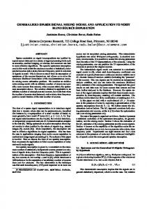
where: Nf is the number of frames where the summand is above −10 dB for SIR gain, and −30 dB for distortion; Sˆ is the estimated signal that contains So contribution of the original signal; X is the mixing at sensor 1, and Si is the input signal of interest at sensor 1. The summands were saturated at +30 dB for SIR gain and +10 dB for distortion. Ideally, SIRgain should be a large positives, whereas distortion should be a large negative. We performed tests on noisy data for which SIR level for each source is approximately -4.7 dB, while noise determines an SNR level for the average voice on a channel of 10 dB. Figure 1 shows plots of the wav files of interest for a run of the algorithm where the mixing parameters were obtained using the algorithm described in [11] (Step 1 of the present approach, assuming at most one source active at any time frequency point), while Π and source estimation parameters were determined using the implementation of the present estimators. Average SIR gains shows a degradation in performance from N = 1 to N = 2, and from anechoic to echoic data (See Fig. 2). However, mean intelligibility scores are best when the number of sources simultaneously active at any time frequency point is N = 2. By increasing the number of active sources from N1 = 1 to N2 = 2, the total noise power in the outputs increases 2 , or 3dB, explaining some of the drop in SIR gain by a factor of N N1 in Fig. 2. We conjecture that the sweet spot in separation is when N is a small fraction of the total number of sources.
0
2
4
6
8 Samples
10
12
14
16 4
x 10
Fig. 1. Example of 8-channel ML algorithm behavior on mixture of noise
and four voices each at approximately −4.7 dB input SIR. The first four plots represent the original inputs. The fifth row gives the mixture on channel 2. The separated outputs are presented in the last four rows.
5. CONCLUSIONS We show that a small number of simultaneously active sources in time-frequency domain is justifiable from a stochastic perspective. This hypothesis, called generalized W-disjoint orthogonality, extends the model studied in [11], and is obtained as an asymptotic approximation in the expansion of the joint pdf of sparse sources.
[8] A. Jourjine, S. Rickard, and O. Yilmaz, “Blind separation of disjoint orthogonal signals: Demixing N sources from 2 mixtures,” in ICASSP, 2000. [9] R. Balan and J. Rosca, “Statistical properties of STFT ratios for two channel systems and applications to blind source separation,” in Proc. ICA-BSS, 2000. [10] S. Araki, S. Makino, A. Blin, R. Mukai, and H. Sawada, “Blind separation of more speech than sensors with less distortion by combining sparseness and ica,” in IWAENC2003, 2003, pp. 271–274. [11] R. Balan, J. Rosca, and S. Rickard, “Scalable non-square blind source separation in the presence of noise,” in ICASSP2003, HongKong, China, April 2003. [12] S. Rickard, R. Balan, and J. Rosca, “Real-time time-frequency based blind source separation,” in Proc. ICA, 2001, pp. 651–656. [13] S. Rickard and O. Yilmaz, “On the W-disjoint orthogonality of speech,” in Proc. ICASSP, 2002, vol. 1, pp. 529–532.