Genesis of the Model ... functions. Shape-Parameter Gamma Weibull GE. 1. 1. 1. 1. > 1. 0 â 1 ... GE is more closer to the gamma distribution rather than the ...
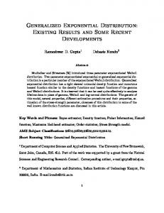
Generalized Exponential Distribution
Debasis Kundu Department of Mathematics and Statistics Indian Institute of Technology, Kanpur India
Joint Work: R.D. Gupta, Univ. of New Brunswick & A. Manglick, Univ. of Umea.
IIT Kanpur
Outline of the Talk • Genesis of the Model • Model Description • Common Properties Gamma Distribution
with
Weibull
and
• Moments of the GED • Inference • Closeness with Other Distributions • Generation of Gamma and Normal Random Variables Using GED • References
IIT Kanpur
Genesis of the Model Gompertz (1825, Phil. Trans. Roy. Soc. Lon.) used the following distribution function to represent mortality growth ¶ µ 1 −λt α t > ln ρ. G(t) = 1 − ρe λ Ahuja and Nash (1967, Sankhya A) also used this model and some related model for growth curve mortality Gupta and Kundu (1999, ANZJS) consider a special case of this model µ
F (x; α, λ) = 1 − e
¶ −λx α
;
x > 0.
This is a special case of the exponentiated Weibull model proposed by Mudholkar and his co-workers (1995, Technometrics)
IIT Kanpur
Model Description Here α is the shape and λ is the scale parameter. It has different shapes of the density function µ
f (x; α, λ) = αλ 1 − e
¶ −xλ α−1 −xλ
e
;
x > 0.
It has different shapes of the hazard functions h(x; α, λ) =
µ
¶ −λx α−1 −λx
αλ 1 − e e f (x; α, λ) = α 1 − F (x; α, λ) 1 − (1 − e−λx )
IIT Kanpur
; x > 0.
Physical Interpretations A parallel system is a system where the system works if at least one of the components works If the shape parameter α is an integer it represents the life time of a parallel system when each component follows exponential distribution
IIT Kanpur
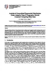
Shapes of the Different Density Functions Since λ is the scale parameter we take λ = 1 1.6
α = 0.50
1.4 1.2 1
α = 1.0
0.8
α = 2.0
0.6
α = 10.0 α = 50.0
0.4 0.2 0
0
2
4
6
IIT Kanpur
8
10
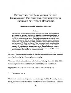
Shapes of the Different Hazard Functions Since λ is the scale parameter we take λ = 1 2
1.5
α = 0.4 α = 0.5
1
α = 1.0 α = 2.0
0.5
α = 5.0 0
0
2
4
6
IIT Kanpur
8
10
Comparisons with Gamma and Weibull Distributions Density Functions • Shape parameter = 1 all are equal to exponential distribution • Shape parameter > 1, all are unimodal • Shape parameter < 1, all are decreasing functions Hazard Functions • Shape parameter = 1 all have constant hazard functions • Shape parameter > 1, all are increasing functions • Shape parameter < 1, all are decreasing functions
IIT Kanpur
Closer look at the hazard functions
Shape-Parameter Gamma Weibull
GE
1
1
1
1
>1
0↑1
0↑∞
0↑1
Here [α] is the integer part of α and < α > is the fractional part of α. Yj ’s are i.i.d. exponential with mean 1 and Z follows GE with shape parameter < α >. E(X) =
1 , i i=1 n X
V (X) =
IIT Kanpur
1 . 2 i i=1 n X
Sum of n i.i.d GE Distribution If X1, . . . , Xn are n i.i.d. GE(α), then the density n X Xi is function of X = i=1
fX (x) =
∞ X
j=0
cj fGE (x; nα + j)
Here
n X
cj > 0
i=1
cj = 1.
If we approximate it by M terms, i.e. fX (x) ≈
MX −1 j=0
cj fGE (x; nα + j),
then the error due to approximations is bounded by
1−
MX −1 j=0
g(x), cj
Explicit expression of g is available. IIT Kanpur
Estimation The problem is to estimate the unknown parameters from a random sample of size n. • The family of the GED satisfy all the regularity conditions • The MLEs work quite well if α is not very close to 0 • Fixed point type iterative process can be used to solve the non-linear equation • If α is close to 0, the iterative process takes longer time to converge • Other estimators like Moment Estimators, L-Moment estimators, Percentile Estimators, Least Squares Estimators, BLUE have been tried
IIT Kanpur
If one of the parameters is known • If the scale parameter is known then the MLE of the shape parameter can be obtained in explicit form • If the shape parameter is known then the MLEs of the scale parameter can be obtained by solving a nonlinear equation. • Other estimators also can be obtained accordingly
IIT Kanpur
Testing and Confidence Intervals • LRT can be used for testing purposes if both are unknown • If λ is known it is an exponential family, then the UMP or UMPU test exists for testing the shape parameter • If α is known then testing the scale parameter LRT can be used • If both the parameters are unknown then asymptotic confidence intervals can be used for constructing confidence intervals • If λ is known then exact confidence intervals based on χ2 distribution is available IIT Kanpur
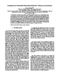
Closeness with Other Distributions For certain ranges of the shape and scale parameters the distribution function of the GE distribution can be very close to the corresponding distribution functions of Weibull, gamma and log-normal distributions.
IIT Kanpur
The distribution function of GE(12.9) and LN(0.3807482, 2.9508672) 1 0.9 0.8 0.7 0.6 0.5 0.4 0.3 0.2 0.1 0
0
2
4
6
IIT Kanpur
8
10
Disadvantage: It is very difficult to distinguish between the two models. Selecting the correct model for small sample sizes becomes almost impossible. Advantage: Log-normal distribution function or gamma distribution function can be approximated very well by GE
IIT Kanpur
We can generate approximate random samples of log-normal ( implies normal also) and gamma distributions using GE A very convenient approximation of the standard normal distribution function can be used as Ã
Φ(z) ≈ 1 − e
! −ezσ+µ 12.9
where σ = 0.3807482
µ = 1.0820991
In this case the error of approximation is less than 0.0003.
IIT Kanpur
Generation of N (0, 1) Using the approximation, approximate N (0, 1) can be easily generated Generation of Gamma(α) Consider the Gamma distribution with the following density function 1 α−1 −x fGA(x; α) = x e ; Γα
x>0
It can be shown that for 0 < α < 1 2α 1 fGE (x; α, ) fGA(x; α) ≤ Γ(α + 1) 2 Using the inequality and by Acceptance-Rejection method gamma random numbers can be generated IIT Kanpur
References • Ahuja, J. C. and Nash, S. W. (1967), “The generalized Gompertz-Verhulst family of distributions”, Sankhya, Ser. A., vol. 29, 141 - 156. • Gompertz, B. (1825), “On the nature of the function expressive of the law of human mortality, and on a new mode of determining the value of life contingencies”, Philosophical Transactions of the Royal Society London, vol. 115, 513 - 585. • Gupta, R. D. and Kundu, D. (1999). “Generalized exponential distributions”, Australian and New Zealand Journal of Statistics, vol. 41, 173 - 188. • Gupta, R. D. and Kundu, D. (2003), “Discriminating between the Weibull and the GE distributions”, Computational Statistics and Data Analysis, vol. 43, 179 - 196. IIT Kanpur
References (cont.) • Gupta, R. D. and Kundu, D. (2005), “Comparison of the Fisher information between the Weibull and generalized exponential distribution”, (to appear in the Journal of Statistical Planning and Inference) • Kundu, D., Gupta, R D. and Manglick, A. (2005),“Discriminating between the lognormal and generalized exponential distribution”, Journal of the Statistical Planning and Inference, vol. 127, 213 - 227. • Raqab, M. Z. (2002), “Inferences for generalized exponential distribution based on record statistics”, Journal of Statistical Planning and Inference, vol. 104, 339 - 350. • Raqab, M. Z. and Ahsanullah, M. (2001), “Estimation of the location and scale parameters of generalized exponential distribution based on order statistics”, Journal of Statistical Computation and Simulation, vol. 69, 109 - 124. IIT Kanpur
References (cont.) • Zheng, G. (2002), “Fisher information matrix in type -II censored data from exponentiated exponential family”, Biometrical Journal, vol. 44, 353 - 357.
IIT Kanpur