Real-time Adaptive Control Using Neural Generalized Predictive Control Pam Haley, NASA Langley Research Center -
[email protected] Don Soloway, NASA Ames Research Center –
[email protected] Brian Gold, Langley Aerospace Research Summer Scholar -
[email protected] Abstract The objective of this paper is to demonstrate the feasibility of a Nonlinear Generalized Predictive Control algorithm by showing real-time adaptive control on a plant with relatively fast timeconstants. Generalized Predictive Control has classically been used in process control where linear control laws were formulated for plants with relatively slow time-constants. The plant of interest for this paper is a magnetic levitation device that is nonlinear and open-loop unstable. In this application, the reference model of the plant is a neural network that has an embedded nominal linear model in the network weights. The control based on the linear model provides initial stability at the beginning of network training. In using a neural network the control laws are nonlinear and online adaptation of the model is possible to capture unmodeled or time-varying dynamics. Newton-Raphson is the minimization algorithm. Newton-Raphson requires the calculation of the Hessian, but even with this computational expense the low iteration rate make this a viable algorithm for real-time control. 1. Introduction Generalized Predictive Control (GPC) belongs to the class of Model-Based Predictive Control (MPC) techniques and was first introduced by Clarke and his co-workers in 1987 [1,2,3]. Linear model predictive control has a long reputation as a powerful control tool in industrial control processes [4,5,6]. However nonlinear model predictive control is still viewed as an academic tool mainly because of the difficulties associated with reliable construction of a nonlinear model [7]. In the predictive control scheme the model is used to predict the future behavior of the system due to both known and unknown input effects. The accuracy of the model prediction directly determines the quality and effectiveness of the control law and is the primary consideration during implementation. The construction of the model can be either derived from fundamental principles, based on empirical data, or, as in this paper, a combination of the two. A detailed discussion about the modeling and identification as it applies to nonlinear model predictive control can be found in [7]. A nonlinear model that is constructed from fundamental principals could be globally valid over the entire input space depending on the assumptions that are made. The derivation can be extremely rigorous and often leads to very high order models, which can introduce complications for real-time computation. Empirical modeling is the process of transforming available input output data into meaningful input output relations. The main limitation of a model based on observations is that the prediction capability is only valid for the region spanned by the data so nothing can be said about the accuracy of the predictions based on extrapolations. The magnetic levitation (MAGLEV) system presents significant challenges for neural network modeling and predictive control. The challenge for the neural network model is online learning for the MAGLEV system. The challenge for the controller is to compute real-time control laws for the MAGLEV system that has dynamics that are considered to be relatively fast, especially for a
MBC scheme. In this paper the neural network model is initialized with a nominal linear model. The control based on the linear model provides initial stability at the beginning of network training. The neural network is then allowed to learn the unmodeled dynamics of the nonlinear plant thus combining fundamental and empirical modeling. This paper also demonstrates the feasibility of this NGPC implementation by establishing real-time control at 500 Hertz while adapting the neural network model online. All results are using a single-input single-output system. In the next section the Experimental Setup will be described followed by discussions of the Neural Generalized Predictive Control, Forming the MAGLEV Model (Fundamental Principles), Neural Network Model, Real-time Adaptive Control, and Conclusions and Recommendations. 2. Experimental Setup The plant to be controlled is a magnetic levitation or MAGLEV device. Magnetic levitation is a means of suspending an object in space by controlling the magnetic force produced by current flowing through a magnetic coil. The MAGLEV device used for this work has two coils that are positioned side by side to suspend two one-inch metal balls in the air by the electromagnetic force due to the DC magnet above it. This device is capable of two degrees-of-freedom (DOF), vertical translation and rotation [8]. The MAGLEV device can be used as a 1DOF single-input singleoutput (SISO) system that commands only vertical translation of a single metal ball or a 2DOF multi-input multi-output (MIMO) system that also produces rotation through two separate vertical translations of two metal balls connected by a nonferrous rod. This paper presents results for the SISO 1DOF MAGLEV device only. The MAGLEV device is comprised of two DC magnets, a current drive system, two light sources, and two photosensors. Each of the DC magnets is made of 3800 turns of gage-22 magnet wire wrapped about a one-inch diameter low carbon steel core that is
Coil Position Sensor
Voltage Lamp
Voltage Ball
Analog Filters
A/D Conversion
Convert to Position
NGPC
Convert to Voltage
Figure 1. Magnetic Levitation System
D/A Conversion
4.5 inches in length. The current drive system includes two ± 45volt power supplies and two power op-amps to regulate the voltage across each coil. Incandescent lights pass light though convex optical lenses to cast a shadow from a suspended metal ball on to arrayed infrared photosensors. Each photosensor array measures positions from 1 to 20 millimeters from the bottom of the core. Figure 1 depicts the MAGLEV device and the block diagram indicating the real-time control system. The MAGLEV device and real-time controller together will be referred to as the MAGLEV system.
The main steps of the NGPC algorithm are: 1)
2) 3) 4) 5)
A voltage signal measuring the position of a metal ball is passed through analog filters (a RC network with 100 Hz roll-off). This sensor measurement is used for feedback control. The analog signal is then digitally sampled at 500 Hz and converted into a position representation, in meters, that is sent to the NGPC algorithm. The NGPC algorithm calculates the next current command, in amps, that will place the metal ball at some specified location. The current command is then converted into an analog voltage signal and sent through a coil drive circuit to a coil.
Starting with the previously calculated control input, u(n), predict the performance of the plant for the specified horizon using the model The value of the horizon is determined through a priori tuning. Calculate a new control input that minimizes the cost function, Repeat steps 1 and 2 until desired minimization is achieved, Send the “best” control input to the maglev as the new u(n), Repeat for each time step.
The cost function used for position control of the MAGLEV system, Equation (1) and Equation (2), has three terms. The first term represents the sum of the mean square error between the desired output and the output of the neural network model. The neural network model serves to predict the plant outputs from N1 to N2 future time steps. The second term is the weighted square of the control increments. The weighting factor, λu, acts to smooth the control inputs. The calculated inputs for the plant predictions form the control increments. They are calculated for Nu future time steps. The only constraint on the values of the horizons is that Nu and N1 be less than or equal to N2.
The NGPC algorithm is implemented in C-code on a Pentium II 400 MHz PC running Windows 95. Data acquisition is performed with a National Instruments E-Series multifunction I/O card. The interface between the control algorithm and the data collection is done using the NI-DAQ library provided with the acquisition card.
J=
N2
2
The block diagram of the Neural Generalized Predictive Control system is shown in Figure 2. It consists of four components: the MAGLEV device, a neural network model for prediction, a tracking signal that specifies the desired position of the suspended metal ball, and the Cost Function Minimization (CFM) algorithm that calculates the current command needed for the magnetic coil to produce the desired position.
Desired Position
Cost Function Minimization (CFM)
Current Command u(n) S
g(u) = Measured Position
s
s
4s
(2)
The third summation of J, Equation (2), defines constraints placed on the control input over a horizon of Nu. The constraint function g(u), is plotted in Figure 3. The first two terms of g(u) form the two sides of the function while the third part insures that the minimum of the function is zero.
z-1 S
Model of Plant (Neural Network)
Nu
∑ u(n + j) − lower + upper − u(n + j) − upper − lower . j =1
y(n)
Magnetic Levitation Plant
j =1
where N1 is the minimum-costing horizon, N2 is the maximum-costing horizon, Nu is the control horizon, ym is the desired tracking trajectory, yn is the predicted output of the model, λu is the control input weighting factor, ∆u(n + j) = u(n + j) − u(n + j − 1) .
A complete derivation of the NGPC algorithm for a general SISO system is developed in [10]. A summary is presented herein.
ym(n)
(1)
2
u
j = N1
3. Neural Generalized Predictive Control
Nu
∑ [ym(n + j) − yn(n + j)] + ∑ λ ( j)[∆u(n + j)] + g(u).
yn(n)
Predicted Position
The sharpness, s, controls the shape of the constraint function while the sides are bounded by upper and lower, the input constraint. The smaller the value of s, the sharper the corners get. In practice s is set to a very small number, for example 10-20. From both the equation and Figure 3 it is easily seen that as the control input, u, approaches either the upper or lower bound, the value of the input constraint function approaches infinity which places a high cost on the minimization of this term. If the minimization produces either u ≤ lower or u ≥ upper then u is set to u + ε or u - ε respectively. The value of ε is set to 10-6 [9].
The NGPC Algorithm
Figure 2. Block Diagram of the NGPC System and Algorithm The NGPC algorithm operates in two modes, prediction and control. Prediction occurs between samples by setting a doublepole/double-throw switch, S, to the neural network model. The NGPC algorithm utilizes the model to predict over some finite horizon, the response of the plant to the inputs calculated by the CFM algorithm. The CFM algorithm minimizes a user specified cost function to calculate the next control input. The NGPC system is set back to a mode of control before the next sample time when the switch is set back to the MAGLEV device. At this time the control input that minimizes the cost function over the entire horizon is passed to the MAGLEV as the current command, u(n). The algorithm used to accomplish this is outlined below.
4279
operating point. Newton's Second Law of motion can be applied in the vertical direction to obtain
1 0.9 0.8
&y& = g −
0.7
g(u)
0.6 0.5
0.3 s 0.2 0.1 -1
-0.5
0
0.5
1
1.5
u lower
(3)
Where f(i,y) is the electromagnetic force on the metal ball due to the electromagnet. The model of this force was determined through experimental calibration. For small air gap devices such as the MAGLEV, it has been experimentally shown that the magnetic field density remains uniform throughout the gap, and that the force experienced due to the electromagnet is of the form [11]
0.4
0 -1.5
1 f (i , y ) . m
upper
2
i . f (i, y) = p(y)
Figure 3. Plot of Input Constraint Function Currently, there is no systematic way to determine the values for the four tuning parameters N1, N2, Nu, and λu, for a nonlinear system. For a linear system the necessary condition to achieve stability is Nu equal to the order of the system while N2 is used to tune for performance. The value for λu should approach zero. Dead time in the system is accounted for with the value of N1.
(4)
It has been empirically observed that p(y) can be modeled using a linear representation of the form a + by, where a and b are constants and y is the vertical distance from the bottom of the coil. Substituting Equation (4) into Equation (3) yields 2
The CFM algorithm used to minimize the cost function is the Newton-Raphson iterative algorithm. Newton-Raphson is a quadratically converging algorithm that requires the calculation of the Jacobian and the Hessian. Although the Newton-Raphson algorithm can be computationally expensive, the low number of iterations needed for convergence makes it a feasible algorithm. The computational issues of Newton-Raphson are addressed in [10].
&y& = g −
1 i . m a + by
(5)
The MAGLEV device is inherently nonlinear due to the inverse square law that reduces the electromagnetic force taken to suspend the metal ball further from the coil. The linear model is generated by linearizing Equation (5) about a nominal operating point, (y0,i0), to obtain
4. Forming the MAGLEV Model (Fundamental Principles)
i by &y& = k 0 − i , a + b y0
The MAGLEV device is open-loop unstable, which presents the challenge of maintaining initial stability of the suspended object while the weights of the neural network are adjusted to “learn” or model the dynamics of this plant. This problem is handled by incorporating a nominal linear model into some of the weights of the neural network while other weights are allowed to learn unmodeled or time varying dynamics of the open-loop system [9].
(6)
Taking the Laplace transform of Equation (6) and substitution of the constants, which are found in Table 1, produces the transfer function
Y (s) −k −25.6796 = = . (7) (s + 39.1546)(s − 39.1546) I (s) s2 − k i0 b a − b y0
Embedding a nominal linear model into the neural network has two key advantages. First, for many open-loop unstable systems, it is often infeasible to let the plant go unstable the number of times it would take the neural network to minimally learn the dynamics enough to stabilize the plant. This method could cause the plant to be damaged or destroyed. Also, incorporating available information about a plant can reduce the training time for the neural network.
The open-loop instability is apparent by the right half plane pole of Equation (7). Table 1. Definition of Constants
k
This section will be used to develop a nominal linear model of the MAGLEV device from the nonlinear equations of motion. The development of this model leaves many of the plant effects unmodeled to demonstrate the ease and feasibility of combining a nominal linear model with the capability of a neural networks to model unmodeled dynamics including nonlinearities. The manner in which the linear equations are embedded into a neural network will be described subsequently.
y0 i0 a b m g b0 b1 b2 a1 a2
A metal ball of mass, m, is placed underneath the electromagnet at a distance, y. The current, i, flowing into the electromagnetic coil will generate electromagnetic force, f, to attract the metal ball. The net force between the gravitational force and the electromagnetic force will cause the metal ball to move up or down. The metal ball is kept in a dynamic balance around an
4280
2 i0 m(a + b y0) 0.01m
2
m g (a + b y0 ) = 0.7640 amps
0.2042 72.988 0.0682 kg 9.81m/s2 0 -0.5138x10⁻⁴ -0.5138x10⁻⁴ 2.0061 -1
This continuous-time model is discretized at a sampling rate of 500 Hz using a zero-order hold approximation yielding the difference equation
y(n) = b0 i (n) + b1 i(n-1) + b2 i(n-2 ) + a1 y(n-1) + a2 y(n-2 ) ,
which is sufficient for learning. The output range of interest is ±0.004m, which is too small for effective training. Consequently, the output of the network was scaled by 0.004. The feedback signal, y(n-1) or yn(n-1), is scaled up by 1/0.004 for the same reason. The embedded linear model is made equivalent to the scaled neural network by scaling each of the input coefficients of Equation (8) by 1/0.004. The scaling on the b terms of the ARMA model is not reflected in Figure 4.
(8)
where the values of the coefficients are given in Table 1. 5. Neural Network Model
For the experiment the network used 3 nonlinear hidden layer nodes in addition to the one linear node associated with the linear model. Four additional time-delays were also added to the input and feedback nodes. The learning gain for the neural network was 0.01.
The neural network architecture that is used for the MAGLEV model is a multi-layer feedforward network (MLFN) with tappedtime delays. The network structure shown in Figure 4 depicts the SISO structure with the linear model embedded into the weights. The current, i, is the input to the MAGLEV system and vertical position, y, is the output. The inputs to the network are current , past values of the current, and the past position measurements of the MAGLEV. The network has a single hidden layer with multiple hidden layer nodes and a single output node. The activation function for the output node is linear with a slope of one and the activation functions for the hidden layer nodes is either linear if the node is associated with the linear portion of the model or the hyperbolic tangent. The linear hidden layer node also has the biases set to zero. y (n-1)
6. Real-time Adaptive Control Results The position of the metal ball is controlled to track a series of filtered pulses of increasing amplitude about the linearized operating point of 10mm. The maximum distance commanded is ± 4mm. This pulse train is continuously repeated during the experiment. The ball is initially placed under the coil and after some period of time, online adaption of the neural network weights is subsequently enabled. Tuning the controller was accomplished by first tuning the parameters in simulation. This initially gave the set of tuning parameters N1 = 1, N2 = 7, Nu = 2, and λ = 0.00001. Starting with these parameters the hardware was retuned to stable operation with N1 = 1, N2 = 15, Nu = 2, and λ = 0.625. The change in N2 is expected by virtue of going from a simulation to hardware, but the difference of the λ term is due to the network scaling. The value for λ changed from 0.00001 to 0.00001(1/0.004)2, or 0.625.
1 0.004
i (n) z
i (n-1) -1
z
b1
b2
~ ~ (n-2) y (n-1) y
i (n-2)
z -1
-1
Adaptable Weights Fixed Weights a1 a 2
Nonlinear Nodes Linear Nodes
1
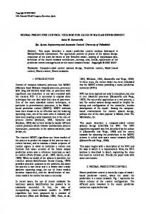
Figure 5 shows the tracking performance of the metal ball relative to the pulse train. The data is displayed by overlaying sections of the pulse train during different time periods in the experiment. The four traces represent the desired tracking reference trajectory, the performance of NGPC using only the nominal linear model, and the performance of NGPC after 20 seconds of training and 60 seconds of training. As the network training continued, a reduction in tracking error due to the decrease in error between the maglev device and the neural network model can be seen.
0* ~ yn (n) 0.004
* - only 0 before training
yn (n)
Figure 4. Neural Network Structure for Embedding Linear Model 0 Ref. Trajectory Before Training 20 Sec. of Training 60 Sec. of Training
To embed the linear model into the network, the weights between the input layer and the linear hidden layer node correspond to the coefficients of the linear ARMA model in Equation (8). The weight from this hidden node to the output node is set to one. The remaining weights going to the nonlinear hidden layer nodes are randomly initialized. The weights coming from the nonlinear nodes to the output node is initially set to zero to prohibit the contribution of the nonlinear portion to the model output until the system is stabilized. Once stability is attained, the training algorithm is turned on until acceptable model accuracy is achieved. The weights associated with the linear model remain fixed throughout training. The backpropagation-training algorithm was used where the weights were updated at each sample. For more information on using neural networks refer to [12, 13, 14].
Figure 5. Reference Trajectory Relative to Various Sections During Network Adaption
Training for the neural network works best if the inputs and output are scaled around ±1. The current ranges between 0.3 to 1 amp,
A running root mean square (RMS) error between ym(n) and y(n), tracking error, over the entire experiment of 600 seconds is shown
Position (mm)
5
10
15
20 0
1
2
3
4
5
6
Time (Seconds)
4281
in Figure 6. Shortly after network training is enabled at 60 seconds, a significant reduction in the RMS error occurred.
[4] C. E. Garcia, D. M. Prett, and M. Morari., “Model Predictive Control: theory and practice – a survey”, Automatica, 25(3):335-348, 1989.
1.10E-03
[5] M. Morari and J. H. Lee, “Model Predictive Control: Past, Present and Future,” PSE97/ESCAPE5, Computers and Chemical Engineering, 1997.
training enabled at 60 seconds
1.00E-03 9.00E-04
[6] S. Joe Qin and T. A. Badgwell, “An Overview of Industrial Predictive Control Technology”, Chemical Process Control – V, Assessment and New Directions for Research, Tahoe City, CA Janurary 1996.
RMS
8.00E-04 7.00E-04 6.00E-04 5.00E-04
[7] J. H. Lee, “Modeling and Identification for Nonlinear Model Predictive Control: Requirements, Current Status and Future Research Needs”, Proceedings of The International Symposium on Nonlinear Model Predictive Control: Assessment and Future Directions, Ascona, Switzerland, 1998.
4.00E-04 3.00E-04 2.00E-04 0
100
200
300
400
500
600
Time (Seconds)
[8] D. Lane, “Linear H∞ Optimal Control of a Two Degree of Freedom Magnetic Suspension System”, Masters Thesis, Drexel University, 1996.
Figure 6. Running RMS Error between ym(n) and y(n) Both sets of results demonstrate the significant performance gain obtained of using the nonlinear neural network to adapt the reference model of the plant.
[9] D. Soloway, “Neural Generalized Predictive Control For RealTime Control”, Masters Thesis, Old Dominion University, 1996.
7. Conclusions and Recommendations
[10] D. Soloway and P. Haley, “Neural Generalized Predictive Control: A Newton-Raphson Implementation,” Proceedings of the IEEE CCA/ISIC/CACSD, IEEE Paper No. ISIAC-TA5.2, Sept. 15-18, 1996.
This paper has demonstrated that the Neural Generalized Predictive Control algorithm is practicable for some SISO applications requiring high sampling rates and real-time computations. The NGPC algorithm has subsequently been implemented for MIMO systems. It is currently being tested for the 2DOF MAGLEV system and on a F-15 Active simulator for 6DOF control.
[11] D. Lane, R. McConnell, and W. S. Gray, “Force Modeling for the Control of a Two-Dimensional Magnetic Levitation System,” Proceedings 1994 IEEE Regional NY/NJ Control Conference, Piscataway, New Jersey, 1994, pp. 149-152. [12] K. S. Narendra and K. Parthasarathy, “Identification and Control of Dynamical Systems using Neural Networks”, IEEE Transactions on Neural Networks, March 1990.
The paper also shows that embedding a nominal linear model into the neural network is a suitable way to solve the problem of training on an open-loop unstable plant. For highly nonlinear plants or plants operating over a large set of conditions, a method of breaking an input space into multiple linear regions is sometimes employed. The method of modeling demonstrated in this paper could be applied using multiple neural networks. This could lead to a reduction in the number of overall regions modeled due to the nonlinear modeling capability of neural networks. A gating neural network can then used to blend the output of the models to obtain the most accurate representation of the plant at that condition. This technique using NGPC is being studied.
[13] S. Haykin, “Neural Networks: A Comprehensive Foundation”, Macmillan Publishing Company, Englewood Cliffs, N. J., 1994. [14] P. D. Wasserman, “Neural Computing – Theory and Practice”, Van Nostrand Reinhold, New York, 1989.
Additional issues that are being studied are concerned with stability properties of the closed-loop system during network adaption and analysis of controller robustness to model uncertainties. References [1] D. W. Clarke, C. Mohtadi and P. C. Tuffs, “Generalized Predictive Control - Part 1: The Basic Algorithm,” Automatica, Volume 23, 1987, pp 137-148. [2] D. W. Clarke, C. Mohtadi and P. C. Tuffs, “Generalized Predictive Control - Part 2: The Basic Algorithm,” Automatica, Volume 23, 1987, pp 149-163. [3] D. W. Clarke, “Advances in model-based predictive control,” in Advances in Model-Based Predictive Control, ed. by D. W. Clarke, Oxford University Press, 1994.
4282