Apr 20, 2012 - P â t´MD,..., ´2D, ´D, 0, D,..., MDu and is supposed to take the value 1. The total number of pilots is N â 2M ` 1. Each frame is periodically padded ...
SUBMITTED TO IEEE JOURNAL ON EMERGING AND SELECTED TOPICS IN CIRCUITS AND SYSTEMS
1
Fast and Robust Parametric Estimation of Jointly Sparse Channels Abstract—We consider the joint estimation of multipath channels obtained with a set of receiving antennas and uniformly probed in the frequency domain. This scenario fits most of the modern outdoor communication protocols for mobile access [1] or digital broadcasting [2] among others. Such channels verify a Sparse Common Support property (SCS) which was used in [3] to propose a Finite Rate of Innovation (FRI) based sampling and estimation algorithm. In this contribution we improve the robustness and computational complexity aspects of this algorithm. The method is based on projection in Krylov subspaces to improve complexity and a new criterion called the Partial Effective Rank (PER) to estimate the level of sparsity to gain robustness. If P antennas measure a K-multipath channel with N uniformly sampled measurements per channel, the algorithm possesses an OpKP N log N q complexity and an OpKP N q memory footprint instead of OpP N 3 q and OpP N 2 q for the direct implementation, making it suitable for K ! N . The sparsity is estimated online based on the PER, and the algorithm therefore has a sense of introspection being able to relinquish sparsity if it is lacking. The estimation performances are tested on field measurements with synthetic AWGN, and the proposed algorithm outperforms non-sparse reconstruction in the medium to low SNR range (ď 0dB), increasing the rate of successful symbol decodings by 1{10th in average, and 1{3rd in the best case. The experiments also show that the algorithm does not perform worse than a nonsparse estimation algorithm in non-sparse operating conditions, since it may fall-back to it if the PER criterion does not detect a sufficient level of sparsity. The algorithm is also tested against a method assuming a “discrete” sparsity model as in Compressed Sensing (CS). The conducted test indicates a trade-off between speed and accuracy. Index Terms—Channel Estimation, Sparse, Finite Rate of innovation, Effective Rank, Krylov Subspace.
I. I NTRODUCTION OMMUNICATIONS between two parties are subject to unknowns: noise and filtering by the Channel Impulse Response (CIR). With respect to decoding, the noise is treated as nuisance parameters, and the CIR coefficients as unknowns to be estimated as precisely as possible to maximize the decoding rate. For this purpose, the channel can be used to transmit a signal known at both ends — the pilots — to gain knowledge about the CIR. It dictates a trade-off between the portion of the channel reserved to the pilots — thus lost to data — and the decoding
C
Y. Barbotin and M. Vetterli are with the faculty of Informatics and ´ Communications at Ecole Polytechnique F´ed´erale de Lausanne, Switzerland This work has been submitted to the IEEE for possible publication. Copyright may be transferred without notice, after which this version may no longer be accessible. This research is supported by Qualcomm Inc., ERC Advanced Grant Support for Frontier Research - SPARSAM Nr : 247006 and SNF Grant - New Sampling Methods for Processing and Communication Nr : 200021-121935/1.
frequency
frequency
time
frequency
time
a) block layout
b) comb layout
time
c) scattered layout
Fig. 1. In pilot assisted OFDM communications, time-frequency slots are reserved (black) for pilots, thus providing a sampling of the CIR in time and frequency. K scatterers
Rx P SCS channels
arXiv:1204.4626v1 [cs.SY] 20 Apr 2012
Yann Barbotin Student Member, and Martin Vetterli, Fellow, IEEE
Tx
... K signal components
Fig. 2. The ideal SCS channel model is a set of P channels of bandwidth B each having K components aligned in time. Assuming complex valued signal components, the total number of unknowns is p2P ` 1qK instead of 3P K for a sparse model with independent time of arrivals (ToA), or 2P times the Nyquist Rate for a bandlimited model.
error rate due to bad channel estimation, both affecting the communication bitrate. The two interdependent aspects of channel estimation are therefore the selection of pilots and the design of an estimation algorithm. We focus on the later and use uniform DFT pilot layouts shown in Fig. 1, which are found in modern communication standards using OFDM. The pilots provide information about the CIR, and so does an priori knowledge about its structure. In the noiseless case, the CIR can be perfectly recovered with a finite set of samples if it perfectly obeys the a priori known structure, thus providing a sampling theorem — e.g. uniform pilots in time at the Nyquist rate characterize uniquely bandlimited signals. In this paper we study Sparse Common Support (SCS) channels, i.e. channels sharing a common structure of very low-dimension. Fig. 2 shows an example of SCS channels. A. Problem definition Imposing a structure may not lead to a trivial linear system of equations as it is the case for Shannon/Nyquist (projection
B. Contributions With these considerations in mind, we adress the estimation of Sparse Common Support (SCS) channels from DFT-domain measurements (pilots). SCS channels estimation with FRI was studied in a previous paper [3], and we hereby focus on computational issues and robustness. A fast algorithm is derived based on Krylov subspace projections. Its main advantage is to have a computation and memory cost proportional to the sparsity level K. It relies on FFT evaluations for the heavy load computations, which is particularly appealing for embedded DSP applications. The sparsity level is unknown in practice, and we derive a heuristic estimate of it using a new measure called the Partial Effective Rank (PER). The PER tracks the “effective dimension” of the Krylov subspace as its size is increased, and can therefore be estimated online unlike other information criteria such as Akaike, MDL [7] or the EDC [8]. To assess the performances of the proposed algorithm, simulations are performed on measured CIRs to which synthetic AWGN is added. We compare the obtained results with an algorithm exploiting discrete sparsity to see if the input shift sensitivity described in Fig. 3 is a practical issue. C. Outline First, we will explicit the SCS channel model for aerial electromagnetic transmissions, and see under which conditions this model is relevant. Our conclusion is that the SCS property may not always be verified, which is confirmed by the data shown in Fig. 4. It establishes the requirements for a robust SCS estimation algorithm aware of the operating conditions. 1 notwithstanding
the limitations of machine precision.
...
...
−1Mag.
1
¨¨
a) Evolution of CIR over time log10
Tunnel
CIR [sample]
150
−2 −3
100
−4 −5
50 −6 0 0
10
20
30
40
50
Time [s] b) From “sparse” to “not so sparse” in 20s t “ 10s
in a linear subspace). The SCS structure is a union of K unidimensional subspaces [4], [3] shared by P channels which leads to an estimation problem exactly and efficiently solvable in the framework of Finite Rate of Innovation sampling [5]. In [3] an estimation algorithm SCS-FRI is proposed and studied. This leads to two questions. First, as seen in Fig. 3.a), the SCS-FRI algorithm selects the K subspaces from an infinite and uncountable set1 which could be sampled. This is the approach taken by Compressed sensing (CS) or the sparse representation literature. The limiting case is to reduce the set to form a basis as shown in Fig. 3.b). The CIR can be perfectly and uniquely represented with elements of this set, but it probably won’t have a K-sparse representation. A possible trade-off is to enlarge the set to form a frame as in Fig. 3.c). Reconstruction becomes more complex, but the shiftinvariance provided by the frame [6] gives a better K-sparse representation. Second, models are an approximation of reality — e.g. Fig. 4 — and it is not immediately clear which amount of modelization error can be tolerated in practice. This is especially important as we rely on a very specific signal structure, and this question can only be answered by trials on field measurements.
¨P
SUBMITTED TO IEEE JOURNAL ON EMERGING AND SELECTED TOPICS IN CIRCUITS AND SYSTEMS
t “ 30s
2
Fig. 4. Field measurements collected in [9]. The receiver is a base-station with P “ 8 antennas, and the transmitter is mobile. The image a) shows the magnitude of the first antenna’s CIR. The channel is qualitatively sparse except when the transmitter goes through a tunnel. The real part of the CIR for three different antennas is shown in b) confirming the common support property and the transient nature of sparsity.
Second, we quickly review the application of FRI and discrete sparse representations to the SCS estimation problem. Details are left out since they are already present in the literature [10], [3], [11]. The third part is devoted to the design of a fast and robust algorithm for the SCS estimation problem, based on Krylov subspace projections with OpKP N logpN qq operations, requiring OpKP N q memory, where K is the number of sparse components, P is the number of channels, and N is the number of collected samples per channel. For robustness, we introduce the Partial Effective Rank (PER) derived from the work of Roy [12], which only adds a marginal OpK 2 q cost to be evaluated online. The PER is used to derive a heuristic estimate of K requiring little overhead. The heuristic may fail if the channel is not sparse enough, giving a beneficial sense of adequacy to the algorithm. In such non-sparse cases, the algorithm can yield to a non-sparse estimation method. The resulting algorithm — combining FRI sampling, the PER criterion and Krylov subspace projection — named FRIPERK was implemented in MATLAB and compares favorably to FRI for N ą 200. We conclude with the application of FRI-PERK and a CS algorithm (RA-ORMP) to field measurements collected in [9] with synthetic AWGN, and compare them with a simple non-parametric method (spectrum lowpass interpolation). The results show the SCS property can be exploited in the medium to low SNR bracket (below 0dB) to significantly lower the Symbol Error Rate (SER). Compared with the non-parametric method, FRI-PERK increases the proportion of correctly decoded symbols by 1{10 in average, and 1{3 at best.
BARBOTIN & VETTERLI: FAST AND ROBUST ESTIMATION OF JOINTLY SPARSE CHANNELS
Model & Acquisition t0 P r0, 1r
T “ 1{N
0 T
c) T {4 nT
t P r0, 1r
0
n ă 4N, P Z
...
...
t0
t0
nT {4
n ă N, P Z
...
1-sparse representation
sinc1{2πT
b)
t
Synthesis functions
c0
a)
3
t0
Fig. 3. Consider a single pulse (´ ´ ´, dashed curve) critically sampled as shown on the left column. From the samples (´ˆ, stems), 1-sparse representations of the original signal are computed. In a), the problem is treated as a parametric estimation of t0 and c0 as in the FRI framework. Conceptually, the signal component is chosen from the infinite and uncountable set of the pulse shape and its shifts in r0, 1r. The original signal has a perfect 1-sparse representation in this setup. In b), the signal component is chosen in a finite set of functions forming a basis of the signal space. The original signal can be represented by these functions, but it does not have a 1-sparse representation in general. In c), three times more synthesis functions are added to the set, to form a frame. The signal has a much closer 1-sparse representation in this frame thanks to the shift invariance introduced by the redundancy between the synthesis functions, but the estimation becomes combinatorially more complex. The estimation frameworks b) and c) are referred as discrete sparsity which is used in Compressed Sensing (CS), and the estimation is subject to a trade-off between accuracy and complexity.
II. T HE PHYSICS OF SPARSE COMMON
SUPPORT CHANNELS
A. Sparsity beyond simulations Algorithms for the estimation of a sparse signal from noisy measurements are quite mature [13], [14], [3]. The principal hurdle for their application to physical signals is the inadequacy between the simple theoretical model and reality. For example, indoor electromagnetic channels are in general not sparse, as described in the Saleh and Valenzuela model [15]. In this model, reflections are bundled in clusters having an exponentially decaying energy. This dynamic holds in general [16], [17], and after demodulation, an electromagnetic channel impulse response hptq can be described as the superposition of clustered reflections, hptq “
K ÿ
ÿ
cl ϕpt ´ tk ´ ∆l q,
k“1 pAl ,∆l qPCk F
ÐÑ
K ÿ
k“1
e´jωtk
ÿ
pAl ,∆l qPCk
Al e´jω∆l ϕpe p jω q,
(1)
such that ϕ is the channel mask in the time domain (after demodulation), and Ck are clusters of reflections with a delay tk . Within each cluster we observe reflections shifted by ∆l from tk with randomly distributed complex-valued2 amplitudes Al . The number of clusters K is usually small, but the total number of reflexions is not. However, if the bandwidth Ωϕ of ϕ and the maximal intra-cluster delays ∆l are small enough, the 0th order approximation e´jω∆l ϕpe p jω q « ϕpe p jω q,
2 After demodulation, the equivalent baseband channel becomes complexvalued.
holds at all considered frequencies ω Ps ´ π, πs. If in addition the amplitudes are distributed identically and independently enough, one of the many avatars of the central-limit theorem may be used to obtain a simplified model known as the “Multipath Rayleigh channel model”: hptq “
K ÿ
k“1
Ck ϕpt ´ tk q,
˘ ` Ck „ NC 0, c2k I .
(2)
The channel is called sparse if and only if the expected delay-spread τ upper-bounding tK ´ t1 verifies K{τ ! Ωϕ {2π, i.e. if the rate of innovation is substantially lower than the Nyquist rate. The requirements for sparsity are thus two-folds: ‚ The “girth” of each cluster must be a fraction of the inverse bandwidth of the channel. ‚ The density of clusters must be a fraction of the channel bandwidth The first property hints at channels with a low or medium bandwidth, while the second one requires long-distances propagation where both the transmitter and receivers are in a relatively clear environment, such as outdoor communications. The high velocity of electromagnetic (EM) waves ensures scatterers of large dimensions, such as trees, generate clusters of modest time spread allowing the use of the simplified model (2) instead of (1) for channels with a bandwidth up to 100M Hz approximately. Fig. 5 summarizes the conditions necessary for the channel to be sparse. The channel shown in Fig. 4 has a bandwidth of 120MHz, and an EM wave travels 2.5m in a time-lapse equal to the inverse-bandwidth. Therefore, in typical noisy operating conditions, reflections having
4
SUBMITTED TO IEEE JOURNAL ON EMERGING AND SELECTED TOPICS IN CIRCUITS AND SYSTEMS
Long delay-spread τ
(a)
(b)
Low bandwidth B{8
High bandwidth B
Short delay-spread τ {8
(c)
(d)
Fig. 5. This figure shows how sparsity relates to the channel bandwidth and its delay-spread. All four panels (a)–(d) have the same number of signal components — 80 of them grouped in 8 clusters with exponentially fast energy decay. Signals (a) and (c) cannot be considered sparse as the rate of innovation is close to/greater than the Nyquist rate on the time-lapse corresponding to the delay-spread, and 0 outside it. Signal (b) is weakly sparse, the rate of innovation is for this reason also high. In this setup the discrete sparsity approach may be suitable. The signal (d) can be considered sparse as only the 8 clusters will be resolvable in the presence of noise. The rate of innovation of this approximation is much lower than the Nyquist rate. Even though (b) and (d) have the same rate of innovation in a strict sense, (d) can be approximated with a signal having 1{10th the rate of innovation of (b) thanks to its low bandwidth. This approximation motivates the use of a model with a low rate of innovation in the low-SNR regime where the model approximation error has less power than the noise.
a path difference of a fraction of 2.5m will be unresolvable. On the other hand the ratio K{τ will be quite large necessitating long range outdoor transmissions for the channel to be considered sparse. Fig. 5 shows the magnitude impulse responses of an outdoor channel with a medium bandwidth from the FTW3 MIMO dataset [9], and confirms this analysis. Note that we do not rule-out the occurrence of sparsity in ultrawide-band communications as the channel dynamics become quite different at very short range [18].
B. Common support We now consider the case where a receiver (Rx) possess several antennas, as in SIMO and MIMO communications. Therefore, if we consider a 1-to-P communication verifying the multipath model (2), the receiver observes P channels hp ptq “
K ÿ
Ck,p ϕpt ´ tk,p q,
p “ 1, . . . , P,
k“1
for a total of 3KP unknown coefficients parametrizing the channels. As for sparsity, the high velocity of EM waves is again a crucial factor to establish the common support property, and 3 Forschungszentrum
Telekommunikation Wien,
http://measurements.ftw.at
the difference in amplitudes tk,1 « tk,2 « ¨ ¨ ¨ « tk,P ,
(3)
Ck,1 ‰ Ck,2 ‰ ¨ ¨ ¨ ‰ Ck,P .
(4)
Indeed, if dmax is the maximal distance between the P receiving antennas, the ToA difference between antennas is upper-bounded by 2dmax {c.The criterion for common support (3) is c . dmax ! π Ωϕ In Fig. 4, dmax “ 60cm and π Ωcϕ “ 1.25m. To assert (4), we need to quantify the spatial correlation of paths amplitudes between the receiving antennas. Using [3] (Proposition 6), and assuming narrow scatterers, the correlation between antennas separated by a distance dm,n can be approximated as ” ı E Ck,m Ck˚1 ,m c ” ı ” ı “ δk´k1 J0 pdm,n ωcarrier {cq . 2 2 E |Ck,m | E |Ck1 ,n |
Using the numbers of Fig. 5, correlation between antennas does not exceed 0.5. In most communication scenario (4) is verified by design as it provides spatial diversity [19]. In conclusion, we see that the common support property is relatively easy to establish as it only depends on the antennas topology. This is not the case for sparsity, in Fig. 4 when the transmitter enters a tunnel, a dense train of reflections is observed. Hence, it is reasonable to say outdoor communications with medium bandwidth have typically —as opposed to “surely”— sparse channel impulse responses.
III. E STIMATION OF
SPARSE COMMON - SUPPORT CHANNELS FROM DFT PILOTS
Assume each frame of period τf is uniformly sampled in time xp rns “ xp pnτf {Nf q ,
n “ 0, . . . , Nf ´ 1.
The pilot layouts in Fig. 1 lead to estimate a set of sparse common support channels from a uniform subset of its DFT coefficients. To make notation less cumbersome, we assume without loss of generality that Nf “ 2M D ` 1 , and use negative indices which shall be understood “modulo the index limit” in general. Also the pilot index is centered on the DC carrier P “ t´M D, . . . , ´2D, ´D, 0, D, . . . , M Du and is supposed to take the value 1. The total number of pilots is N “ 2M ` 1. Each frame is periodically padded to ensure the convolution with the CIR is circular, thus pp, p p “ diag p1P q h x
ô xp “ W diag p1P q W H hp , such that W is the DFT matrix, 1P is the indicator of P,
BARBOTIN & VETTERLI: FAST AND ROBUST ESTIMATION OF JOINTLY SPARSE CHANNELS
and p hp rns “
K ÿ
nt {τ Ck,p WNfk s .
(5)
k“1
is the sampled SCS channel model in the DFT domain. The operator W diag p1P q W H is the orthogonal projection in the subspace spanned by the basis vectors of the DFT corresponding to the pilot indices. With a good synchronization, the ToAs are contained in s ´ τ {2, τ {2s, and if Yτ ] s D ď , D P N, (6) τ p p can be recovered by ideal lowpass the original spectrum h interpolation H
H
W hp “ C D diag p1P q W xp ,
5
is an pM `1qˆK Vandermonde matrix and J is the exchange matrix. This decomposition has the merit to clearly show T p has a column-space of dimension K which depends only on the support, and is thus the same for each channel. Moreover any basis for this column-space verifies a rotation invariance property. Indeed, let def
Then V Ò “ V ÓΨ ,
Any basis V having the same span as V can be written as def V “ VA, where A is a fullrank K ˆ K matrix, therefore V Ò “ V Ò A,
(7)
sinpπpm ´ nq{Dq . sinpπpm ´ nq{Nf q
This principle is at the core of OFDM communications which interleave data and pilots in the DFT domain. If the measurements xp are corrupted by AWGN, this technique projects orthogonally the measurements in the signal subspace and therefore minimizes the estimation MSE if common-support property or sparsity are ignored. A. FRI approach The channels in (5) do not lie in linear subspaces, but in a common union of subspace. Therefore the channels can be estimated in two-steps 1) Identify jointly the K subspaces (the common support). 2) Compute the orthogonal projection of the measurements in the union of subspaces separately for each channel. Algorithms and analysis for this problem are found in [3], and are a simple extension of well-known linear array-processing techniques such as ESPRIT [20] or the annihilating filter [21] to common-support channels. The union of subspaces is identified by studying the columnspace of the following data matrices » fi p hp r0s p hp r´Ds p hp r´2Ds ¨ ¨ ¨ — ffi —p p p hp r0s hp r´Ds ¨ ¨ ¨ffi — hp rDs ffi ffi, Tp “ — —p p p hp r0s ¨ ¨ ¨ffi —hp r2Ds hp rDs ffi – fl .. .. .. .. . . . . of dimensions pM ` 1q ˆ pM ` 1q These data matrices have a Vandermonde decomposition T p “ J Vdiag pCp,1 , . . . , Cp,K q V H , » fi 1 ¨¨¨ 1 — ffi — W Dt1 {τs ¨ ¨ ¨ W DtK {τs ffi — ffi ffi such that V “ — —W 2Dt1 {τs ¨ ¨ ¨ W 2DtK {τs ffi , — ffi – fl .. .. .. . . .
and V Ó “ rVs2:M,: .
´ ¯ Ψ “ diag W Dt1 {τs , . . . , W DtK {τs .
“ V Ó ΨA, Ó “ loVomo Aon looomooon A´1 ΨA .
such that C D is circulant with entries rC D sm,n “
def
V Ò “ rVs1:pM´1q,:
VÓ
X
which means the support is recovered from any basis V of the column-space of T p as the phase of the eigenvalues of the solution to V Ò “ V ÓX , which is the ESPRIT algorithm [20]. In the presence of AWGN, the basis V may be obtained in a robust manner from the SVD of the stacked matrix » fi T1 — ffi — . ffi T “ — .. ffi , (8) – fl TP
but other subspace identification techniques may be used depending on the measurements model. To compare with the canonical estimation technique (7), this method not only uses the limited-length of the delayspread but also sparsity and common-support. The solution of the estimation problem is to be found in a smaller set of candidates. We expect that with good algorithms the estimation will be more resilient to noise. On the other hand more restrictive models yield higher modelization error. Note that sparsity is not used to reduce the number of pilots but to make the estimation more robust to noise. See [3] for pilot reduction. B. CS approach
p p corresponding to the set of The measured DFT samples x pilot subcarriers P are linked to the channel impulse response coefficients by X “ rW sP,C H, def
(9) def
X “ rrp x1 sP , . . . , rp xP sP s , H “ rh1 , . . . , hP s , where C is the index set on which the channel impulse responses are supported a priori. C contains contiguous indices covering a time-lapse less than or equal to the delay-spread.
6
SUBMITTED TO IEEE JOURNAL ON EMERGING AND SELECTED TOPICS IN CIRCUITS AND SYSTEMS
The matrix of channel coefficients H is assumed to be jointly row-sparse, i.e. only a few rows of H are not null. This is known as the MMV (Multiple Measurement Vectors) problem which is not a trivial extension of the SMV (Single Measurement Vector) problem. It has received a lot of attention in the past few years and good, efficient algorithms exist such as RA-ORMP [13], Lee & Bressler [14],. . . First notice that the channel model described in (5) is not jointly row-sparse nor sparse, unless the ToAs coincide with the sampling points. Second, since (6) holds, the system (9) is invertible, which is typically not the case in compressed sensing. In this study sparsity is used as a regularization technique to gain robustness to noise as in Section III-A. One could select a random subset of pilots to effectively compress the channel measurements leaving additional space for data. The compressed sensing literature on sparse channel estimation has followed two tracks 1) The ToA coincide with the sampling grid. 2) The ToA do not coincide with a regular grid resulting in “approximately sparse” channels [11], [10], [22]. It introduces a model mismatch which can be mitigated using frames (increased estimation complexity). The first assumption is remote from reality and the reported performances shall be taken with a grain of salt, nevertheless it is useful to benchmark algorithms. The second one is more relevant and its limitations due to model mismatch may fade away when applied to real-world data where it is unavoidable anyway. IV. A PPLICATION OF
THE
FRI
APPROACH :
PERK
In this section, we consider the number of signal components K and the number of antennas P to be small compared to the number of pilots N . The FRI based channel estimation technique outlined in Section III-A has two shortcomings if implemented in a straightforward manner 1) Its computational complexity and memory footprint are respectively OpN 3 q and OpN 2q . Both are contributed by the SVD decomposition used to estimate the columnspace of T . 2) The sparsity level K is unknown. The complexity 1) is especially important for channel estimation as it is a core signal processing block at the receiver’s physical layer. It is called on several times per second, and must operate in real-time with limited power and hardware resources. A. An O pKP N log N q FRI estimation Naive computation of an SVD of T defined in 8 to obtain a K-dimensional subspace of the column-space is wasteful for two reasons. First, only K out of M ` 1 principal singular pairs pσm , v m are of interest. Second, T is well structured — made of Toeplitz blocks — and matrix factorization techniques such as QR will destroy this structure during the factorization process, rendering it unexploitable and requiring an explicit storage of the data matrix.
Since we are interested in the column-space of T , we will work on the hermitian symmetric correlation matrix T HT “ “
P ÿ
TH p T p,
p“1
which has eigenpairs pσm , v m , m “ 0, . . . , M . A solution to compute only the leading eigenpairs, is to project the correlation matrix in a Krylov subspace [23]. This is an iterative method in which computations are performed on the original matrix, meaning the original structure is preserved. Hence the memory footprint is kept low and the computational complexity is similar for each iteration. Krylov approximants have received a lot of attention in the numerical analysis [23], [24], [25], [26] or control theory [27], [28] literature, therefore we will only quickly skim through the subject. Projection into a Krylov subspace is done with Lanczos algorithm. A comprehensive analysis was done by Xu [29] for the estimation of covariance matrices in linear array processing. He proposed an OpN 2 q algorithm4 together with an approximate OpN 2 q estimation of the subspace dimension K. Implementation of the Lanczos algorithm is quite involved in practice and may require costly corrections at each iteration [26], [23], [24], this is why asymptotically more expensive OpN 3 q are generally preferred unless the system is very large. The additional structure on the original data matrix T allows us to lower the complexity from OpN 2 q to OpN log N q, making it appealing even for matrices of modest size, and we will derive a novel criterion to estimate the signal subspace dimension K which requires OpK 2 q computations to be run along the subspace estimation process. A K-dimensional Krylov subspace K of a M -dimensional hermitian matrix A has is KK,f pAq “ spank“1,...,K Ak f , where f is an initial vector which can be randomly chosen. Note that all the properties of Krylov subspaces only hold in probability, an “unlucky” initial draw may compromise them. The k th basis vector Ak f is a monomial of A of degree k, therefore using a three terms linear recursion on this sequence of monomials one can derive a sequence of orthogonal polynomials [33]. This is equivalent to say that an orthonormal basis QK of KK,f pAq is computed by orthogonalization of each of Ak f only against the two previous ones and normalization. So, the main cost of the procedure is the computation of the non-orthogonal basis vectors, which is done by recursive matrix-vector multiplications. The three terms recursion used to orthogonalize the Krylov basis implies that KK,f pAq has a tridiagonal decomposition Pf ,K A “ QH K ΓK QK . where QK is unitary and ΓK is symmetric and tridiagonal (thanks to the 3-terms recursion). The eigenpairs of Pf ,K A are derived from this factorization at little cost [23], [24], and they are called the Ritz pairs. 4K
is considered small and constant compared to N and P “ 1.
BARBOTIN & VETTERLI: FAST AND ROBUST ESTIMATION OF JOINTLY SPARSE CHANNELS
7
TABLE I A PPROXIMATIVE “O” COMPLEXITY FOR SUBSPACE IDENTIFICATION . Algorithm
Main computation
Storage
Latency
Processing units (pu)
KP N log N P N3 P N3
KpN ` 1q P N2 P N2
KN [30] P N3 N plog N ` P q
P ˆ FFT engines (N ` 1 points) 1 multipurpose pu. N 2 ˆ 2-by-2 SVD pu.
Krylov + PER Full SVD (serial) Full SVD (systolic array) [31], [32]
The full SVD is done with Jacobi rotations and can be massively parallelized using the systolic array method of Brent, Luk & Van Loan [31]. Parallelism greatly reduces the latency of the system, but since it does not reduces the number of computations it comes at the cost of using multiple processing units.
A remarkable property is that the Ritz pairs quickly converge to the principal eigenpairs of A as K grows. This quick convergence does not follow exactly the result of Xu [29] — since in our case the Toeplitz blocks are of approximately square size — but it can be explained with a theorem of Saad [23] (Theorem 12.4.1) which links the rate of convergence of the Ritz pairs to the growth rate of Chebyshev polynomials. The theorem shows that Ritz pairs converge faster to the corresponding eigenpairs if the eigenvalues are farther apart. Because of the Toeplitz structure of the data matrix, matrixvector multiplications with T H T , which is the central step of a Lanczos iteration has a cost of OpP N logpN qq. Indeed, T HT f “
P ÿ
TH p T pf
p“1
is the sum of P matrix-vector multiplications, each of them realized as two consecutive Toeplitz maxtrix-vector multiplications. Square Toeplitz matrices of dimension M `1 can be embedded in circulant matrices of dimension 2pM ` 1q “ N ` 1 ff « s def T p T p , Cp “ Tsp T p T p “ toeplitzptp,´M , . . . , tp,0 , . . . , tp,M q,
T p “ toeplitzptp,1 , . . . , tp,M , 0, tp,´M , . . . , tp,´1 q.
Circulant matrices are diagonalized by the DFT matrix, hence the cost of a circulant matrix-vector multiplication is dominated by the cost of 4 FFT. Since ff « « ff ı ” IM OM f H H Cp “ T HT f, IM OM C p OM OM 0 each Lanczos iteration has a cost dominated by 4P FFT5 of length N ` 1. Since only the first half of the input and the first half of the output of each FFT are non 0 or not needed, each FFT could be replaced by two FFT of half the size. The resulting algorithm fulfill all the requisites for a fast embedded implementation since most of the computational load is put on the FFT block, ubiquitous in communication systems. Table I B. On-line sparsity assessment
working online with the Lanczos algorithm. Its main advantage compared to other methods is to require little information about the noise space. A formal study of the PER is deferred to an upcoming report. 1) Shortcomings of traditional information criterions: Information theoretic criteria such as Rissanen’s MDL [7], Akaike criterion or the EDC [34] are powerful mathematical tools which may be used to evaluate the sparsity level K. They all follow a similar pattern, which is to minimize ITCpσ, Kq “ Lpσ, Kq ` K ¨ p2pM ` 1q ´ Kq ¨ PpM q, where L is the log-likelihood function based on σ the singular values of T , and K an estimate of the sparsity level. The term P is a penalty growing at rate between Op1q and opN q depending on which one of the criteria is used. Their performances are well understood [35], but the evaluation of the likelihood function requires to compute the product M ź
m“K
2 σm
H
“ detpT T q
O
K´1 ź
σk2 ,
k“0
which has an algorithmic cost superior to the Lanczos algorithm itself. Also, the argument used in [36] to show consistency of a partial evaluation of ITCpσ, Kq cannot be used in our setup because the asymptotic distribution of the noise matrix spectrum6 is extremely different. As the number of pilots increases, the probability measure of the noise spectrum concentrates [37], but its support is unbounded. This is a major difference with the setup considered in [36], [29] where the noise power spectrum concentrates around the noise variance . Formally we can say Proposition 1: Let T be an pM ` 1qP ˆ pM ` 1q matrix composed of fixed and finite number P of stacked Toeplitz blocks T p of square dimensions pM ` 1q ˆ pM ` 1q as in (8). Assuming the generators of each block are sequences of white Gaussian noise σmax pT H T {pM ` 1qq “ Oplog M q, i.e. even with proper normalization, the spectral norm of an all-noise matrix diverges. Proof: The matrix norm induced by the euclidian vector
In this section we introduce the Partial Effective Rank (PER) a criterion to estimate the signal subspace dimension 5 The
DFT of the circulant generators can be precomputed.
6 “spectrum” shall be understood as the SVD spectrum of the matrix and not the noise Fourier power spectrum when matrices are concerned.
8
SUBMITTED TO IEEE JOURNAL ON EMERGING AND SELECTED TOPICS IN CIRCUITS AND SYSTEMS
a) 1
(10)
We then use a result of Meckes [38] on the spectral norm of square Toeplitz matrices with independently distributed subgaussian generating coefficients ´a ¯ }T 1 } „ O M log M . (11)
0.7
0.5
true sparsity level 0.4
Hpp1 , . . . , pM q “ ´
M ÿ
pm loge pm .
20
30
40
50
60
64
dB
EQgain
A posteriori optimal K Heuristic based on PER (median)
14
10
12
Kest
10 8
true value, K “ 7
5
underestimate 0
6 4
−5 2 −15
−10
−5
0
5
10
SNR [dB] c) 25
FRI + PER (L=5) FRI + K=7 (a priori knowledge) FRI + Oracle (upper−bound) No equalization (equi−SNR)
20
output SNR [dB]
where H is the entropy of the singular values distribution
10
b)
m “ 1, . . . , M.
erankpAq “ eHpp1 ,...,pM q ,
1
K
which together with (10) and (11) proves the proposition.
The Effective Rank of A is
SNR: 9dB
0.6
p
It indicates that for pure AWGN measurements the spectrum of the matrix is unbounded, and one cannot expect the signal and the noise spectrum to separateś nicely. Without a proper 2 approximation, the computation of M m“K`1 σm would have 2 7 a cost of OpP N logpN qq in general , driving the complexity of the algorithm. 2) The Partial Effective Rank: The effective rank, is a matrix functional introduced by Roy [12] which may be seen as a “convexification” of the rank. Definition 1: Let A be a matrix with singular values σ “ rσ1 , . . . , σM sT in decreasing order, and singular values distribution
4dB
0.8
Using the triangle inequality and Meckes´ result ÿ }T H T } ď }TpH Tp } „ P OpM log M q,
pm “ σm {}σ}1 ,
´6dB ´11dB ´1dB
0.9
PERK
norm on CpM`1qP is submultiplicative, therefore ›« › ff › IM`1 O ” ı› › › }T 1 } ď › T O › ď 1 ¨ }T }. › O › O
15
10
5
m“1
For elementary properties of the effective rank, we defer to [12]. We can now introduce the partial effective rank Definition 2: For A and H as in Definition 1 and pK,k “ σk {}σ1:K }1 ,
k “ 1, . . . , K ď M,
the Partial Effective Rank (PER) is PERK pAq “ eHppK,1 ,...,pK,K q . The PER verifies Proposition 2:
0 −10
−8
−6
−4
−2
0
2
4
6
8
10
input SNR [dB] Fig. 6. Simulation on a signal with 7 components. The PER curves in (a) show a clear inflection at K “ 7. As the SNR diminishes, the inflection occurs at lower values of K and completely disappears at SNRs ă ´10dB. The graph b) empirically shows that the PER indicates the number of components significantly above noise level which can be reliably estimated: the value of K it predicts follows (in median) the one minimizing the channel estimation error (energy of the residual). Finally, in c) the estimation performances obtained with the PER closely follow the one obtained with an oracle choosing a posteriori the optimal number of components. We see also that below ´5dB the underestimation of K by the PER is beneficial compared to the true value 7. At high SNR, the PER sometimes overestimate the number of paths, mitigating the performances.
0 ď PERK`1 pAq ´ PERK pAq ď 1. The lower bound 0 is reached if and only if σK`1 “ 0 and the upper bound 1 if and only if σ1 “ σ2 “ ¨ ¨ ¨ “ σK`1 . 7 Using a block-Levinson recursion to estimate the determinant T , it maybe brought down to OppP N q2 q, but it was not verified.
The increase of the partial effective rank with K reflects how “significant” is the K th principal component of A compared to the previous ones. Fig. 6 provides empirical evidences that the evolution of the PER during the Lanczos process provides a suitable criterion to estimate K.
BARBOTIN & VETTERLI: FAST AND ROBUST ESTIMATION OF JOINTLY SPARSE CHANNELS
We settle on a very simple heuristic to estimate K based on the PER. We choose the smallest K such that 1 PERK pT q ´ pPERK`1 pT q ` ¨ ¨ ¨ ` PERK`L pT qq ď 0, L which is a very simple “positive slope” detector. It introduces a small overhead: K ` L dimensions are required to decided if the signal space is of dimension ď K. Despite its simplicity and its heuristic motivations, this criterion proved to be robust in practice as shown in Fig. 6. Too many components and/or large modelization error indicate the channels are not sparse. V. N UMERICAL
RESULTS
A. accuracy: FRI vs CS vs lowpass 1) Setup: We use the “FTW rural” dataset to compare aforementioned algorithms on the SCS channel estimation problem. The transmitter is a mobile single antenna device8. The receiver is a “base-station” with P “ 8 receiving antennas. A total of 251 frames are transmitted on a 120M Hz wide channel with a 2GHz carrier frequency. The transmission has a high SNR, so we consider the samples to be the ground truth (infinite SNR). Various SNR conditions are simulated with the addition of AWGN to the samples. The DFT pilots are uniformly laid-out every D “ 3 DFT bin. The estimated channel is used to demodulate 4-PSK coded data symbols occupying the left over DFT bins, and the obtained Symbol Error Rate is the quality metric used to benchmark the estimation. 2) Interpretation of the results: From Fig. 7 we may conclude that ‚
‚ ‚
‚
The channels do not exactly fit the SCS model, therefore the modelization error becomes larger than the noise at high SNR The SCS property helps in lowering the symbol error rate at medium to low SNR (below 0 dB) The “sparsity” model assumed by FRI (few reflections) match the field measurements better than the one assumed by CS (few non-0 coefficients) as seen in Fig. 8. Any algorithm exploiting sparsity must be “introspective”, i.e. it must detect when sparsity does not occur, and fall-back to a more traditional method whenever it happens. It is exemplified by the stroll through the tunnel.
B. Computational benchmark Both FRI-PERK9 and RA-ORMP were implemented in MATLAB10 . Because of the decimation in frequency and the limitation of the delay-spread in time, the projection in RA-ORMP cannot be realized with simple FFTs, results are reported in Fig. 9.(c-d). 8 Only
the first Tx antenna is used. the ARPACK library [39]. Since the size of the Krylov subspace dimension must be fixed beforehand, it does not has the ability to stop before Kmax is reached. 10 v. R2011b for MacOS X, running on a 1.8GHz Intel Core I7 processor and enough 1.3 GHz DDR3 memory 9 Uses
9
If this is not the case, we implemented a fast version of it and reported results in Fig. 9.(a-b). Note that such a setup does not apply to most standards [1], [2]. Definitive conclusions for hardware implementations cannot be drawn from these experiments, however we can see that the low asymptotic complexity of FRI-PERK is not misleading since it provides improvements for a number of pilots which are encountered in practice [1], [2] (higher bandwidth modes). For small numbers of pilots, the direct implementation maybe faster, though we did not used the tracking capacity of Lanczos algorithm used by choosing an initial vector lying in the signal space obtained at the previous step [36]. VI. C ONCLUSION In this study, we addressed computational and robustness issues of FRI techniques applied to channel estimation. The tests conducted on field measurements show the SCS assumption is relevant at medium to low SNR where the noise power exceeds the one of model mismatch, and can be used to substantially lower the SER. The PER criterion used to estimate the sparsity level gives satisfactory results, but an upcoming thorough analytical study is required. Comparison with discrete techniques from compressed sensing indicate a trade-off between speed and accuracy compared to FRI-PERK. Using a finer discretization (frames) allows one to vary this trade-off, and shall be tested in the future. We believe that with a proper discretization similar speed/accuracy results shall be met. R EFERENCES [1] G. T. . V9.0, Requirements for E-UTRA and E-UTRAN, ETSI Std., 2009. [2] ETSI, 300 744, DVB; Framing, channel coding and modulation for digital terrestrial television, ETSI Std. 300 744, Rev. 1.4.1, 01 2001. [Online]. Available: http://www.etsi.org [3] Y. Barbotin, A. Hormati, S. Rangan, and M. Vetterli, “Estimation of Sparse MIMO Channels with Common Support,” submitted to IEEE Trans. Commun., 2012. [4] Y. Lu and M. Do, “Sampling Signals from a Union of Subspaces,” IEEE Signal Process. Mag., vol. 25, no. 2, pp. 41 –47, march 2008. [5] T. Blu, P. L. Dragotti, M. Vetterli, P. Marziliano, and L. Coulot, “Sparse Sampling of Signal Innovations,” IEEE Signal Process. Mag., vol. 25, no. 2, pp. 31–40, 2008. [6] A. Aldroubi and K. Gr¨ochenig, “Nonuniform sampling and reconstruction in shift-invariant spaces,” SIAM review, pp. 585–620, 2001. [7] J. Rissanen, “Modeling by shortest data description,” Automatica, vol. 14, no. 5, pp. 465–471, 1978. [8] L. C. Zhao, P. R. Krishnaiah, and Z. D. Bai, “On detection of the number of signals in presence of white noise,” Journal of Multivariate Analysis, vol. 20, no. 1, pp. 1–25, 1986. [9] H. Hofstetter, C. Mecklenbr¨auker, R. M¨uller, H. Anegg, H. Kunczier, E. Bonek, I. Viering, and A. Molisch. (2002). [Online]. Available: http://measurements.ftw.at/MIMO.html [10] C. Berger, S. Zhou, J. Preisig, and P. Willett, “Sparse channel estimation for multicarrier underwater acoustic communication: From subspace methods to compressed sensing,” IEEE Trans. Signal Process., vol. 58, no. 3, pp. 1708–1721, 2010. [11] G. Taubock and F. Hlawatsch, “A compressed sensing technique for OFDM channel estimation in mobile environments: Exploiting channel sparsity for reducing pilots,” in ICASSP 2008, 2008, pp. 2885–2888. [12] O. Roy and M. Vetterli, “The Effective Rank: A Measure of Effective Dimensionality,” in European Signal Processing Conference (EUSIPCO), 2007, pp. 606–610. [13] M. Davies and Y. Eldar, “Rank awareness in joint sparse recovery,” Arxiv preprint arXiv:1004.4529, 2010.
10
SUBMITTED TO IEEE JOURNAL ON EMERGING AND SELECTED TOPICS IN CIRCUITS AND SYSTEMS
a) Average over time (all snapshots)
b) Average over SNR (´15dB to 0dB)
0.55 0.6
SER
0.50 0.45
0.4
FRI-PERK
0.40
Lowpass interp. 0.2
0.35
RA-ORMP
0.30 0 −15
tunnel
0.25 −10
−5
0
0
10
20
SNR [dB]
30 Time [s]
40
50
Fig. 7. From a) we conclude that sparse recovery lowers the SER compared to non-sparse recovery below 0dB of SNR. If we look at the SER over time in b), we see that FRI-PERK is robust in the sense that if the input signal is not sparse, its performs approximately as well as a non-sparse recovery. x 10
0.8
magnitude
b)
a)
−4
1
FRI-PERK estimation
original CIR
0.6
c)
RA-ORMP estimation
noisy measurements
noisy measurements
0.4
noisy measurements
original CIR
original CIR
0.2
0
0
100
200
300
400
150
200
250
150
200
250
Time [sample] Fig. 8. This figure compares the estimation result of FRI-PERK and RA-ORMP. The input signal is the first frame received at the first antenna corrupted with AWGN to obtain ´5dB of SNR. Panel (a) shows the measurements and the original CIR. Panel (b) shows a portion of interest of the CIR estimated with FRI-PERK. The PER criterion estimates K “ 3, and by visual inspection the three signal components found match the largest ones of the original signal. Panel (c) shows the result obtained with RA-ORMP. The discrete sparsity model causes the estimation to be more sensitive to uncorrelated noise, as spurious spikes contributed by noise are estimated as signal components.
[14] K. Lee, Y. Bresler, and M. Junge, “Subspace Methods for Joint Sparse Recovery,” IEEE Trans. Inf. Theory, vol. PP, no. 99, p. 1, 2012. [15] A. Saleh and R. Valenzuela, “A Statistical Model for Indoor Multipath Propagation,” IEEE J. Sel. Areas Commun., vol. 5, no. 2, pp. 128 –137, february 1987. [16] D. Baum, J. Hansen, and J. Salo, “An interim channel model for beyond3G systems: extending the 3GPP spatial channel model (SCM),” in Vehicular Technology Conference, 2005. VTC 2005-Spring. 2005 IEEE 61st, vol. 5. IEEE, 2005, pp. 3132–3136. [17] J. Salz and J. Winters, “Effect of fading correlation on adaptive arrays in digital mobile radio,” IEEE Trans. Veh. Technol., vol. 43, 1994. [18] D. Cassioli, M. Win, and A. Molisch, “The ultra-wide bandwidth indoor channel: from statistical model to simulations,” IEEE J. Sel. Areas Commun., vol. 20, no. 6, pp. 1247 – 1257, aug 2002. [19] T. S. Rappaport, Principles of Wireless Communications, 2nd ed. Upper Saddle River, NJ: Prentice Hall, 2002. [20] R. Roy and T. Kailath, “ESPRIT-Estimation of Signal Parameters Via Rotational Invariance Techniques,” IEEE Trans. Acoust., Speech, Signal Process., vol. 37, pp. 984–995, 1989. [21] D. Tufts and R. Kumaresan, “Estimation of frequencies of multiple sinusoids: Making linear prediction perform like maximum likelihood,” Proceedings of the IEEE, vol. 70, no. 9, pp. 975– 989, 1982. [22] M. Soltanolkotabi, M. Soltanalian, A. Amini, and F. Marvasti, “A
[23] [24] [25] [26] [27] [28]
[29]
[30] [31]
[32]
practical sparse channel estimation for current OFDM standards,” in ICT ’09., may 2009, pp. 217 –222. B. Parlett, The symmetric eigenvalue problem. SIAM, 1998, vol. 20. G. Golub and C. van Van Loan, Matrix Computations. The Johns Hopkins Uni. Press, 1996. Y. Saad, “On the rates of convergence of the Lanczos and the blockLanczos methods,” SIAM J. on Num. Analysis, pp. 687–706, 1980. C. Paige, “Computational variants of the Lanczos method for the eigenproblem,” IMA J. of Applied Math., vol. 10, no. 3, p. 373, 1972. D. Boley and F. Luk, “A general vandermonde factorization of a Hankel matrix,” Int’l Lin. Alg. Soc.(ILAS) Symp. on Fast . . . , 1997. Boley, “Fast identification of impulse response modes via Krylov space methods,” in Decision and Control, 1997., Proceedings of the 36th IEEE Conference on, 1997, pp. 4384–4388. G. Xu, H. Zha, G. Golub, and T. Kailath, “Fast algorithms for updating signal subspaces,” IEEE Trans. Circuits Syst. II, vol. 41, no. 8, pp. 537– 549, 1994. W. Yeh and C. Jen, “High-speed and low-power split-radix FFT,” IEEE Trans. Signal Process., vol. 51, no. 3, pp. 864–874, 2003. R. Brent, F. Luk, and C. Van Loan, “Computation of the singular value decomposition using mesh-connected processors,” Journal of VLSI and computer systems, vol. 1, no. 3, pp. 242–270, 1985. J. Cavallaro and F. Luk, “CORDIC Arithmetic for an SVD Processor,” J. of parallel and dist. computing, vol. 5, no. 3, pp. 271–290, 1988.
BARBOTIN & VETTERLI: FAST AND ROBUST ESTIMATION OF JOINTLY SPARSE CHANNELS
11
Equalization gain
Execution time 1
30
10
FRI-PER
(a)
(b)
0
SNR gain [dB]
−1
10
−2
10
FRI-PERK
Contiguous pilots
10
Time [s]
2ˆRA-ORMP
25
20
FRI-PERK
fast RA-ORMP
15
10
4ˆfast RA-ORMP fast RA-ORMP
−3
10
50
100
150
200
250
300
350
400
450
5 50
500
2
10
10
250
300
350
400
450
500
450
500
FRI-PERK 2ˆRA-ORMP
SNR gain [dB]
25
0
10
−1
10
−2
10
−3
150
200
250
300
350
400
20
RA-ORMP 15
10
FRI-PERK 100
Scattered pilots
Time [s]
200
(d)
FRI-PER
RA-ORMP
50
150
30
(c)
1
10
100
450
500
M ` 1 (half number of pilots)
5 50
100
150
200
250
300
350
400
M ` 1 (half number of pilots)
Fig. 9. A benchmark is run for pilot sequences of length 2M ` 1 “ 101 to 2M ` 1 “ 1001. The top row compares FRI-PERK with FRI-PER — same algorithm using a full SVD instead of Krylov subspace projection — and a fast implementation of RA-ORMP using FFTs, which is possible since the pilots are contiguous in frequency (D “ 1). The bottom row follows the same procedure, but with scattered pilots (D “ 3) and a delay-spread smaller than the frame length. There is no straightforward fast implementation of RA-ORMP in this case. [33] G. Szeg¨o, Orthogonal polynomials. Revised ed. American Mathematical Society (AMS), 1939. [34] Y. Yin and P. Krishnaiah, “On some nonparametric methods for detection of the number of signals,” IEEE Trans. Acoust., Speech, Signal Process., vol. 35, no. 11, pp. 1533–1538, 1987. [35] M. Kaveh, H. Wang, and H. Hung, “On the theoretical performance of a class of estimators of the number of narrow-band sources,” IEEE Trans. Acoust., Speech, Signal Process., vol. 35, no. 9, pp. 1350–1352, 1987. [36] G. Xu, R. H. Roy, and T. Kailath, “Detection of number of sources via exploitation of centro-symmetry property,” IEEE Trans. Signal Process., vol. 42, no. 1, pp. 102–112, 1994. [37] W. Bryc, A. Dembo, and T. Jiang, “Spectral measure of large random Hankel, Markov and Toeplitz matrices,” The Annals of Probability, vol. 34, no. 1, pp. 1–38, 2006. [38] M. Meckes, “On the spectral norm of a random Toeplitz matrix,” Elec. Comm. in Proba., vol. 12, pp. 315–325, 2007. [39] R. Lehoucq, D. Sorensen, and C. Yang, ARPACK users’ guide: solution of large-scale eigenvalue problems with implicitly restarted Arnoldi methods. Siam, 1998, vol. 6.
Yann Barbotin was born in Ambilly, France in 1985. He received the B.Sc. and M.Sc. degrees in Communication Systems from the Swiss Federal Institute of Technology, Lausanne (EPFL) in 2006 and 2009, respectively. As an intern at Qualcomm Inc. in 2009 and an ongoing scientific collaboration he is the co-inventor of five patents on sparse sampling. He is now a PhD candidate in the LCAV laboratory at EPFL. His research interests are in fundamental limitations of estimation problems and sampling.
Martin Vetterli Martin Vetterli was born in 1957 and grew up near Neuchatel. He received the Dipl. El.- Ing. degree from Eidgenossische Technische Hochschule (ETHZ), Zurich, in 1981, the Master of Science degree from Stanford University in 1982, and the Doctorat es Sciences degree from the Ecole Polytechnique Federale, Lausanne, in 1986. After his dissertation, he was an Assistant and then Associate Professor in Electrical Engineering at Columbia University in New York, and in 1993, he became an Associate and then Full Professor at the Department of Electrical Engineering and Computer Sciences at the University of California at Berkeley. In 1995, he joined the EPFL as a Full Professor. He held several positions at EPFL, including Chair of Communication Systems and founding director of the National Competence Center in Research on Mobile Information and Communication systems (NCCR-MICS). From 2004 to 2011 he was Vice President of EPFL and since March 2011, he is the Dean of the School of Computer and Communications Sciences. He works in the areas of electrical engineering, computer sciences and applied mathematics. His work covers wavelet theory and applications, image and video compression, self-organized communications systems and sensor networks, as well as fast algorithms, and has led to about 150 journals papers. He is the co-author of three textbooks, with J. Kovacevic, ”Wavelets and Subband Coding” (PrenticeHall, 1995), with P. Prandoni, ”Signal Processing for Communications”, (CRC Press, 2008) and with J. Kovacevic and V. Goyal, of the forthcoming book ”Fourier and Wavelet Signal Processing” (2012). His research resulted also in about two dozen patents that led to technology transfers to high-tech companies and the creation of several start-ups. His work won him numerous prizes, like best paper awards from EURASIP in 1984 and of the IEEE Signal Processing Society in 1991, 1996 and 2006, the Swiss National Latsis Prize in 1996, the SPIE Presidential award in 1999, the IEEE Signal Processing Technical Achievement Award in 2001 and the IEEE Signal Processing Society Award in 2010. He is a Fellow of IEEE, of ACM and EURASIP, was a member of the Swiss Council on Science and Technology (2000-2004), and is an ISI highly cited researcher in engineering.