GENERATING CONTOUR PLOTS USING MULTIPLE ... - Fumin Zhang

To Appear in 2005 IEEE Swarm Intelligence Symposium

1

GENERATING CONTOUR PLOTS USING MULTIPLE SENSOR PLATFORMS Fumin Zhang and Naomi Ehrich Leonard Department of Mechanical and Aerospace Engineering Princeton University Princeton, NJ 08544 { fzhang, naomi}@princeton.edu ABSTRACT We prove a convergent strategy for a group of mobile sensors to generate contour plots, i.e., to automatically detect and track level curves of a scalar field in the plane. The group can consist of as few as four mobile sensors, where each sensor can take only a single measurement at a time. The shape of the formation of mobile sensors is determined to minimize the least mean square error in the estimates of the scalar field and its gradient. The algorithm to generate a contour plot is based on feedback control laws for each sensor platform. The control laws serve two purposes: to guarantee that the center of the formation moves along one level curve at unit speed; and to stabilize the shape of the formation. We prove that both goals can be achieved asymptotically. We show simulation results that illustrate the performance of the control laws in noisy environments. 1. INTRODUCTION A planar scalar field can be represented approximately by a set of level curves which forms a contour plot. Contour plots for height, depth, temperature and concentration are frequently used in geology and meteorology. When the field is difficult to express in an explicit mathematical form, a contour plot can help us understand the structure of the field. If only fixed sensor platforms are employed, obtaining a contour plot over a relatively large area will require a noticeably large number of platforms. New technology such as satellite remote sensing or airborne surveillance can greatly improve the efficiency. The central idea is to use these moving sensor platforms to automatically scan a large area from a distance. In this context, motion plans for the sensor platforms to cover an area are usually pre-defined. After the plans are executed, level curves are plotted “off-line” by interpolating the collected data. This is similar to running an “edge detection” algorithm on an image. Resolution of the plot is This work was supported in part by ONR grants N00014–02–1–0826, N00014–02–1–0861 and N00014–04–1–0534.

limited by the large distance between the platforms and the area being scanned. Therefore, it is difficult to detect and measure small scale time-varying features, such as a vortex in a fluid field. In some contexts, it is possible to put mobile sensors right in the field to be measured. For example, underwater vehicles can serve as mobile sensors for ocean sampling. Further, computing and communication resources may be available to allow real-time feedback and on-line motion planning. Accordingly, we suggest a more “adaptive” approach towards a fully automated process for generating a contour plot. Our approach is inspired by the recent developments in cooperative control and obstacle avoidance as described in [14]-[17]. We command multiple sensor platforms to work cooperatively and distributively to estimate level curves and to move along any given level curve. The multiple platforms move together in a formation with shape determined by the need to minimize estimation error. The trajectory of the center of the formation tracks a level curve at unit speed. After one level curve is finished, the formation automatically searches for another one and starts the tracking again. This process can be repeated until the entire region is traversed. The algorithm is based on a control law which serves two purposes: to guarantee that the center of the formation moves along one level curve at unit speed, and to stabilize the shape of the formation. We prove that both goals can be achieved asymptotically. We illustrate, with a simulation, the performance of the control law in a noisy environment. Other researchers have developed level curve tracking algorithms, e.g., [5, 10], based on active contour models or the so-called snake algorithms in computer vision [6]. However, in [5] and [10], a large number of sensor platforms are employed and estimates of derivatives up to fourth order are required. Our approach differs from these algorithms in many respects. While it is assumed in [5, 10], for instance, that each platform can measure a gradient estimate, we assume that each platform can only take a single measurement at a time and gradients need to be computed collectively.

2. k r2 − rc k = k rc − r1 k = a and k r3 − rc k = k rc − r4 k = b,

Further, we prove convergence of our control laws. Convergence has not been proved, although it has been observed in many cases, for control laws based on the active contour models.

we get a set of simple equations for estimates. Without loss of generality, suppose the x-axis is aligned with r2 − r1 and the y-axis is aligned with r3 − r4. We let

2. ESTIMATION OF GRADIENTS

rc =

r1 + r2 + r3 + r4 . 4

(1)

zc

=

Dcx

=

Dcy

=

e1 ex ey

z(r1 ) =

r3 a

z(r2 ) = z(r3 ) =

Dcx

z(r4 ) =

r2 x

Dcy

r4

(4)

= zc − z(rc ) = Dcx − ∂x z(rc ) = Dcy − ∂y z(rc ) .

(5)

1 z(rc ) − a ∂xz(rc ) + a2 ∂xx z(rc ) 2 1 2 z(rc ) + a ∂xz(rc ) + a ∂xx z(rc ) 2 1 2 z(rc ) + b ∂yz(rc ) + b ∂yy z(rc ) 2 1 z(rc ) − b ∂yz(rc ) + b2 ∂yy z(rc ) . 2

(6)

We then subtract equations (6) from equations (3) and use (2) to get

Dc

Figure 1. A symmetric arrangement of the formation to simplify the equations for estimating ∇z(rc ). We design a and b to get the minimum mean square error in estimates zc for z(rc ), and Dc for ∇z(rc ).

n1

=

n2

=

n3

=

n3

=

1 e1 − a ex − a2 ∂xx z(rc ) 2 1 e1 + a ex − a2 ∂xx z(rc ) 2 1 e1 + b ey − b2 ∂yy z(rc ) 2 1 2 e1 − b ey − b ∂yy z(rc ) . 2

(7)

Therefore, the errors are known as

Based on the methods suggested in [12], we note that by arranging the four platforms in a symmetric formation as shown in Figure 1 so that: 1. r2 − r1 is perpendicular to r3 − r4 and

z1 + z2 + z3 + z4 4 z2 − z1 2a z3 − z4 . 2b

Next, by using the Taylor series expansion, we obtain second order approximations

y

r1

(3)

A natural question to ask is how to choose the value of a and b to get the most accurate estimates zc and Dc . To find the answer, we first define the errors in the estimates as

where ni ∼ N (0, σ 2 ) is i.i.d. Gaussian noise. We want to find an estimate zc for z(rc ) and an estimate Dc for ∇ z(rc ).

rc

zc − Dcx a zc + Dcx a zc + Dcy b zc − Dcy b

where Dc = (Dcx , Dcy ). This yields the estimates as

Then we assume that the measurement taken by the ith platform is zi = z(ri ) + ni (2)

b

= = = =

z1 z2 z3 z4

Let z(x, y) denote a smooth scalar function in the plane. The points where the gradient of z vanishes are called singular points; all others are called generic points. The set of singular points can have complicated topology. For example, it is possible that a level curve contains both generic and singular points, and some singular points may not belong to any level curve. Although the singular points carry interesting, sometimes very important, information about the field, they often belong to a set of very small measure. In this paper, we concentrate on level curves that contain purely generic points. We employ four moving sensor platforms with their positions denoted by ri ∈ R2 , i = 1, 2, 3, 4. Let rc be the center of the formation i.e.

2

e1

=

ex

=

n1 + n2 + n3 + n4 1 2 + (a ∂xx z(rc ) + b2∂yy z(rc )) 4 4 n2 − n1 2a

=

ey

n3 − n4 . 2b

given there and here in equation (13) require that we know ∂xx z(rc ) and ∂yy z(rc ). In [13], this difficulty was handled by assuming the Hessian of z to be a random matrix with known distribution. Here, we give an algorithm to estimate ∂xx z(rc ) and ∂yy z(rc ). Let Hxx be the estimate for ∂xx z(rc ) and Hyy be the estimate for ∂yy z(rc ). We design another estimator which gives b c , Hxx and Hyy as follows: b zc , D

(8)

We see that the errors are random variables. The mean square error for estimation is L = E[e21 + e2x + e2y ] σ2 σ2 σ2 1 = + 2 + 2 + (a2 ∂xx z(rc ) + b2∂yy z(rc ))2.(9) 4 2a 2b 16 To minimize this mean square error, we let

z1

∂L ∂L = 0 and =0. ∂a ∂b

(10)

z2

This yields the following two equations

z3

4σ 2 + a∂xxz(rc )(a2 ∂xx z(rc ) + b2∂yy z(rc )) = 0 a3 4σ 2 − 3 + b∂yyz(rc )(a2 ∂xx z(rc ) + b2∂yy z(rc )) = 0 b

z4

−

We then obtain

(11)

b cx D

which have a solution if and only if

∂xx z(rc ) ∂yy z(rc ) > 0 .

(12) and

This solution is a∗ =

∗

b =

4σ 2

p (∂xx z(rc ))2 + |∂xx z(rc )| ∂xx z(rc ) ∂yy z(rc )

!

a ∂xx z(rc ) + b ∂yy z(rc ) = 0 .

(17)

(18)

3. ESTIMATION OF CURVATURE OF A LEVEL CURVE A level curve is a curve r(s) parametrized by s such that z(r(s)) is a constant for all values of s. Suppose the gradient ∇z does not vanish along the curve. We define y1 (s) =

(14)

∇z(r(s)) . k ∇z(r(s)) k

(19)

Then at any given point, the unit tangent vector to the curve, denoted by x1 (s), satisfies

We can then increase the values of a and b until one of the upper bounds is reached. Second, suppose one of the second order derivatives vanishes. For example ∂yy z(rc ) = 0. Then a has an optimal value as  1 3 2σ ∗ a = (15) |∂xx z(rc )| and b∗ can be chosen to be the upper bound for b. Other cases can be treated as in the above cases. A similar procedure was used in [13] to find the optimal shape for a formation of three platforms. Both the results

=

z2 − z1 2a z3 − z4 , 2b

(16)

b c . We will not distinguish these two in We see that Dc = D the future. Equation (18) is very useful. If we can estimate Hxx , then we are able to get an estimate of Hyy . In the next section, we show that Hxx can be obtained by estimating the curvature of the level curve passing through rc .

If the condition in equation (12) is not satisfied, there are several possibilities. First, suppose ∂xx z(rc ) > 0, ∂yy z(rc ) < 0 and (a2 ∂xx z(rc ) + b2 ∂yy z(rc )) ≥ 0. Then the optimal solution is that a and b go to infinity. However, as a and b get large, we have to consider the error caused by the third or higher order terms in the Taylor series expansion. Instead of dealing with this difficulty, we impose an upper bound on the value of a and b. One possible strategy is to let 2

b cy D

=

b2 Hyy − a2Hxx = (z3 + z4 ) − (z1 + z2 ) .

1 6

!1 6 4σ 2 p .(13) (∂yy z(rc ))2 + |∂yy z(rc )| ∂xx z(rc ) ∂yy z(rc )

2

b cx a + 1 a2 Hxx = b zc − D 2 1 b = b zc + Dcx a + a2 Hxx 2 b cy b + 1 b2 Hyy = b zc + D 2 1 b = b zc − Dcy b + b2 Hyy . 2

x1 (s) · y1 (s) = 0 .

(20)

We choose the direction of x1 (s) to form a right handed frame with y1 (s) so that x1 and y1 lie in the plane of the page and the vector x1 × y1 points towards the reader. If s is the arc length along the level curve, then we have the following Frenet-Serret equations [11]:

3

dx1 (s) ds

= κ (s)y1 (s)

5. Let y1J , y1K and y1c denote the unit vectors along the directions of the gradient DJ ,DK and Dc . Define

r2 rF

r3

rK

rc Dc

rE DE

DK

r4

=

−κ (s)x1 (s) ,

∇z(rc ) · x1 = 0

DE . k DE k

= = =

zJ + DJ · (r1 − rJ ) zJ + DJ · (r3 − rJ ) zJ + DJ · (r4 − rJ ) .

d dx1 ∇z(rc ) · x1 + ∇z(rc ) · =0. ds ds

(28)

xT1 ∇2 z(rc )x1 + k ∇z(rc ) k y1 · κ (s)y1 = 0

(29)

∂xx z(rc ) + k ∇z(rc ) k κ (s) = 0 .

(30)

This suggests that we can obtain Hxx , the estimate for ∂xx z(rc ), by Hxx = − k Dc k κc . (31) 4. FORMATION CONTROL In order to get accurate estimates for a level curve, we control the four platforms in a symmetric formation as shown in Figure 1. In addition, the vector r2 − r1 should be aligned with the tangent vector to the level curve at the center. In this section we design a formation control law to achieve all these goals. We view the entire formation as a deformable body. The shape and orientation of this deformable body can be described using a special set of Jacobi vectors, c.f. [14, 15, 8, 9, 3] and the references therein. Jacobi vectors are also used for studying the three body problem as indicated in [4], [2] and other standard textbooks. Here, assuming that all platforms have unit mass, we define the set of Jacobi vectors as

(22)

(23)

3. Estimate DJ by solving the following equations: z1 z3 z4

(27)

where ∇2 z(rc ) is the Hessian of z at rc . Because x1 is the unit vector along the x-axis, we have

2. Along the positive or negative direction of DE , we may find the point rJ where zJ = zc using rJ = rE + (zc − zE )

(26)

This implies

(21)

1. Consider the formation formed by r1 , r3 and r4 as shown in Figure 2. Obtain the estimates zE and DE at the center rE of this three platform formation by solving the following equations: = zE + DE · (r1 − rE ) = zE + DE · (r3 − rE ) = zE + DE · (r4 − rE ) .

(25)

along the level curve, we have

where κ (s) is defined as the curvature of the level curve. With a formation of four moving sensor platforms, we are able to estimate κ (s) for the level curve at the center of the formation by the following procedure:

z1 z3 z4

arccos(y1J · y1c ) k rJ − rc k arccos(y1K · y1c ) k rK − rc k .

One important factor for an accurate estimate κc is that the point rE be as close to the point rJ as possible, and similarly for rF and rK . This requires that we place the symmetric four platform formation so that r1 − r2 is tangent to the level curve. With this configuration, because

Figure 2. Detection of a level curve using four sensor platforms. rc denotes the center of the entire formation. rE denotes the center of the formation formed by r1 , r3 and r4 . rF denotes the center of the formation formed by r2 , r3 and r4 . rJ and rK are located on the same level curve as rc .

dy1 (s) ds

= = = =

Obtain the estimate for κ (s) at rc as   1 δ θL δ θR κc = + . 2 δ sL δ sR

DJ

rJ

r1

δ θL δ sL δ θR δ sR

(24)

4. Repeat the previous steps for the formation consisting of r2 , r3 and r4 with appropriate changes in the subscripts for points rF and rK as shown in Figure 2.

q1 4

=

1 √ (r2 − r1 ) 2

q2

=

q3

=

1 √ (r3 − r4) 2 1 (r4 + r3 − r2 − r1 ) . 2

u3

3 1 1 4 k r˙ i k2 = (4 k r˙ c k2 + ∑ k q˙ i k2 ) . ∑ 2 i=1 2 i=1

5. MOTION OF THE CENTER (33) The system equation for the center is:

This allows us to separate the motion of the center from the shape and orientation changes. Lagrange’s equations for the formation in the lab frame are simply the set of Newton’s equations: r¨ i = fi ,

r¨ c = fc .

= uj = fc

(34)

=

f2

=

f3

=

f4

=

1 1 fc − √ u1 − u3 2 2 1 1 fc + √ u1 − u3 2 2 1 1 fc + √ u2 + u3 2 2 1 1 fc − √ u2 + u3 . 2 2

We now let

u2

=

k r˙ c k r˙ c fc · . α

(40)

α˙ = vc .

(41)

vc = −k4 (α − 1) .

(42)

r˙ c . α

(43)

We define a unit vector y2 as a vector perpendicular to x2 but forming a right handed frame with x2 so that x2 and y2 lie in the plane of the page and the vector x2 × y2 points towards the reader. We then define the steering control uc =

(37)

1 fc · y 2 . α2

(44)

Using the facts that fc = (fc · y2 )y2 and x2 · y2 = 0, we have the following equations: dx2 dt dy2 dt

a∗

−k1 (q1 − √ x1 ) − k2q˙ 1 2 b∗ −k1 (q2 − √ y1 ) − k2q˙ 2 2

=

x2 =

where x1 and y1 are tangent and normal vectors for the level curve at point rc , and a∗ and b∗ are given by equation (13) where ∂xx z(rc ) and ∂yy z(rc ) are replaced by estimates Hxx and Hyy . Assuming that x1 and y1 are slowly varying, a simple controller is =

vc

(36)

q1 (t) →

u1

=

It is easy to see that α will converge to unit speed exponentially with a rate determined by k4 > 0. With the speed of the center under control, we now design the steering control for the center so that it will track a level curve. We define the unit velocity vector x2 as

We now design the control forces u1 , u2 and u3 so that as t → ∞, a∗ √ x1 2 b∗ q2 (t) → √ y1 2 q3 (t) → 0

α

Then the equation for speed control is

(35)

where j = 1, 2, 3 and u j and fc are equivalent forces satisfying f1

(39)

This equation describes the motion of the center in the lab frame. Therefore, the motion of the center of mass can be controlled by designing the force fc . We now define the speed α and its controlled rate of change vc as

where fi is the control force for the ith platform for i = 1, 2, 3, 4. In terms of the Jacobi vectors, these equations are equivalent to q¨ j r¨ c

(38)

where k1 , k2 and k3 are positive, constant, scalar gains. It is proved that this controller achieves equation (37) asymptotically with an exponential rate of convergence by following an approach suggested in [14]. Next, we design fc so that the center of the the formation will track a level curve.

(32)

Together with the vector for the center rc , these Jacobi vectors define a coordinate transform which decouples the kinetic energy of the entire system i.e. K=

= −k1 q3 − k3 q˙ 3

=

uc α y2

=

−uc α x2 .

(45)

Next, we observe that the motion along the level curve is 5

ν=

ds = α x2 · x1 . dt

(46)

We design our control law to be

Then we can rewrite equations for x1 , y1 parametrized by t as, dx1 dt dy1 dt

θ θ uc = κ cos θ − 2 fe(z) k ∇z k cos2 ( ) + sin( ) . 2 2

= κν y1 = −κν x1 .

We have the following claim:

(47)

Proposition 6.1 Suppose the scalar field satisfies k ∇z(r) k 6= 0 except for a finite number of points rsup where z(rsup ) = zmin or z(rsup ) = zmax . Under the steering control law given in equation (52), we have θ → 0 and z → C asymptotically if the initial value θ (t0 ) 6= π and r(t0 ) 6= rsup . Proof Let a Lyapunov candidate function be

For convenience, we introduce a variable θ ∈ (−π , π ] such that cos θ

=

sin θ

=

x1 · x2

x1 · y2 .

(48)

By taking the derivative with respect to time on both sides of the first equation in equations (48), we have − sin θ θ˙

=

dx1 dx2 · x2 + x1 · dt dt

=

(κν )y1 · x2 + x1 · α uc y2

=

−κα cos θ sin θ + α uc sin θ .

θ V = − log cos2 ( ) + ℏ(z) . 2

V˙

(49)

(50)

for sin θ 6= 0. When sin θ = 0, we can take derivatives of both sides of the second equation in equations (48). We get the same expression as (50). On the other hand, along the trajectory of the center, the value of z satisfies dz dt

= = =

=

sin θ2 ˙ e θ + f (z)˙z cos θ2 sin θ2

=

α

=

−α

cos θ2

f (z)α k ∇z k sin θ (κ cos θ − uc ) − e

sin2 θ2 cos θ2

(51)

Our goal is to design the tracking control uc so that θ → 0 and z → C asymptotically where C is a constant.

θ˙ |sin θ =0 = 2α fe(z) k ∇z k ,

6. DESIGN OF THE TRACKING CONTROL

2

We let zmin < zmax both be the suprema for the scalar field; they are allowed to be infinity. Let fe(z) be the derivative function of a function ℏ(z) so that the following assumptions are satisfied: (A1) dℏ/dz = fe(z), where fe(z) is a Lipschitz continuous function on (zmin , zmax ), so that ℏ(z) is continuously differentiable on (zmin , zmax ); (A2) fe(C) = 0 and fe(z) 6= 0 if z 6= C;

(A3) limz→zmin ℏ(z) = ∞, limz→zmax ℏ(z) = ∞, and ∃e z such that ℏ(e z) = 0.

.

(54)

Therefore, if α > 0 we have V˙ ≤ 0. The value of the Lyapunov function does not increase. Because our initial condition is such that cos θ (t20 ) 6= 0, it is impossible for cos θ 2(t) = 0 at any time instant t since otherwise V goes to infinity. By the invariance theorem for non-autonomous systems as shown in [7], we conclude that sin θ2 → 0 as t → ∞. θ (t) will not go to π because we have shown that cos θ 2(t) 6= 0. This implies that θ (t) → 0 as t → ∞. Therefore, θ˙ must vanish as t → ∞. Since

∇ z · α x2

α k ∇z k y1 · x2 −α k ∇z k sin θ .

(53)

Then using (50) and (51), its derivative is

Therefore

θ˙ = α (κ cos θ − uc )

(52)

6

(55)

we know that either fe(z) = 0 or k ∇z k = 0. When k ∇z k = 0, we know r = rsup . According to our assumption, V goes to infinity at r = rsup . Thus if we start with r(t0 ) 6= rsup , we must have k ∇z k = 6 0 for all time t > t0 . Therefore, the only possibility left is fe(z) = 0 which implies that z = C. A linearization of the controlled system equations for θ and z reveals that near θ = 0 and z = C, the rate of convergence is exponential. No further analytical result has been obtained about the rate of convergence when the initial conditions are sufficiently far away from θ = 0 and z = C. However, we have observed reasonably fast convergence in our simulations.

10

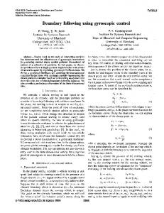
signed simulations for the level set tracking algorithm to test its ability and evaluate its performance in the presence of noise. We allow each sensor platform to obtain information including its own position and measurements of the environment as well as those from other platforms. This assumption is partly ensured by the GPS system and the communication network available at Monterey Bay. Each platform computes the estimates and the control independently. In the planned experiments, there will be significant time delay in the communication links and GPS systems which may cause problems. Therefore, we want each platform to have the ability to compute the behaviors of the entire formation as a starting point for further research to address these problems. Our first step is to test on simple scalar fields with added Gaussian noise. We show one of our simulation results here. The field is generated by placing two identical positive charges at coordinates (5.05, 0) and (−5.05, 0). The added Gaussian noise has a variation as large as 5% of measurements. During the simulation the center of mass (COM) of the formation is first commanded to track the level curve where z = 3.6, which is indicated by the yellow curve in Figure 3. When time is equal to 50 units, it is commanded to track the level curve where z = 4.0, which contains two closed curves inside the yellow curve in Figure 3.

8

6

4

2

0

−2

−4

−6

−8

−10

−10

−5

0

5

10

Figure 3. A snapshot of tracking an artificial scalar field. The yellow line is the level curve for z = 3.6. The level difference between two adjacent level curves is 0.4. The blue and green lines are trajectories of two platforms. The cross symbol indicates the current position of the formation center of mass (COM) .

7. SIMULATION AND PLANNED EXPERIMENTS The level set tracking algorithm is applicable to adaptive sampling using sensor networks in the ocean. Adaptive ocean sampling is a central goal of our collaborative Adaptive Sampling and Prediction (ASAP) project supported by the Office of Naval Research (ONR) [1]. The next planned ASAP field experiment will take place in August 2006 in Monterey Bay, California. A score of gliders and propelled underwater vehicles will be employed to carry on a series of scientific experiments for oceanographic research.

1.8

1.6

1.4

1.2

1 5

0.8 4.5 0.6 4 0.4

0

10

20

30

40

50

60

70

80

3.5

Figure 5. The value of “a”, one of the two shape variables, as function of time. 3

2.5

2

0

10

20

30

40

50

60

70

80

Figure 4. The estimate zc versus time.

In preparation for the planned field experiments, we de-

7

The field and the trajectory of two platforms of the formation are plotted in Figure 3. The small circles with tails represent the platforms and the cross symbol represents the COM. Figure 4 shows the value of the estimate zc of the field z at the COM as a function of time. The mean value is zc = 3.72 for the first level curve and zc = 4.12 for the second level curve. There are clearly errors in the estimates.

The main reason for such errors is that our estimator for z(rc ) is a biased estimator. Further research is underway to improve this estimator. Figure 5 shows how the value of a is adjusted during the process. The first peak is insignificant because the formation has not been fully set up. After the first peak, we see peaks when t is about 12, 36 and 60. At these time instances, the COM is near the line of symmetry where x = 0. Near this line, the second order derivatives of the field have large variations. These results and other results we have observed confirm the theoretical analysis and also suggest that the algorithm is reasonably robust to noise.

[7] H.K. Khalil. Nonlinear Systems, 3rd Ed. Prentice Hall, New Jersey, 2001. [8] R. Littlejohn and M. Reinsch. Internal or shape coordinates in the n-body problem. Physical Review A, 52(3):2035–2051, 1995. [9] R. Littlejohn and M. Reinsch. Gauge fields in the separation of rotation and internal motions in the n-body problem. Reviews of Modern Physics, 69(1):213–275, 1997. [10] D. Marthaler and A. L. Bertozzi. Tracking environmental level sets with autonomous vehicles. In S. Butenko, R. Murphey, and P.M. Pardalos, editors, Recent Developments in Cooperative Control and Optimization. Kluwer Academic Publishers, 2003.

8. ACKNOWLEDGMENT Our control law is motivated from previous work in cooperative formation control and obstacle avoidance found in [15] and [16], where algorithms for tracking a smooth boundary curve are developed and justified. The estimation technique, which provides estimates of second-order derivatives and meets the needs of the control laws, is a natural extension of the adaptive sampling algorithms introduced in [13]. This paper also provides inspiration for our approach to optimizing the formation that minimizes estimation error. In addition, the first author would like to thank Dr. Francois Lekien for suggestions and discussions.

[11] R. S. Millman and G. D. Parker. Elements of Differential Geometry. Prentice-Hall, 1977. [12] P. Ogren, E. Fiorelli, and N. E. Leonard. Formations with a mission: Stable coordination of vehicle group maneuvers. In Proc. of 15th Int’l Symposium on Math. Theory of Networks and Systems, 2002. [13] P. Ogren, E. Fiorelli, and N. E. Leonard. Cooperative control of mobile sensor networks: Adaptive gradient climbing in a distributed environment. IEEE Transaction on Automatic Control, 49:8:1292–1302, 2004.

9. REFERENCES

[14] F. Zhang. Geometric Cooperative Control of Formations. PhD thesis, University of Maryland, 2004.

[1] Adaptive Sampling and Prediction (ASAP) Project. http://www.princeton.edu/˜dcsl/asap/.

[15] F. Zhang, M. Goldgeier, and P. S. Krishnaprasad. Control of small formations using shape coordinates. In Proc. of 2003 International Conference of Robotics and Automation, pages 2510–2515, Taipei, Taiwan, 2003. IEEE.

[2] R. Abraham and J.E. Marsden. Foundations of Mechanics. Second Edition. Addison-Wesley, 1978. [3] V. Aquilanti and S. Cavalli. Coordinates for molecular dynamics: Orthogonal local system. Journal of Chemical Physics, 85(3):1355–1361, 1986.

[16] F. Zhang, E. Justh, and P. S. Krishnaprasad. Boundary following using gyroscopic control. In Proc. of 43rd IEEE Conference on Decision and Control, pages 5204–5209, Atlantis, Paradise Island, Bahamas, 2004. IEEE.

[4] E. Belbruno. Capture Dynamics and Chaotic Motions in Celestial Mechanics. Princeton University Press, Princeton, NJ, 2004.

[17] F. Zhang, A. O’Connor, D. Luebke, and P. S. Krishnaprasad. Experimental study of curvature-based control laws for obstacle avoidance. In Proceedings of 2004 IEEE International Conference on Robotics and Automation, pages 3849–3854, New Orleans, LA, 2004. IEEE.

[5] A. L. Bertozzi, M. Kemp, and D. Marthaler. Determining environmental boundaries: Asynchronous communication and physical scales. In V. Kumar, N. Leonard, and A.S. Morse, editors, Cooperative Control, A Post-Workshop Volume: 2003 Block Island Workshop on Cooperative Control, pages 35–42. Springer, 2005. [6] M. Kass, A. Witkin, and D. Terzopolous. Snakes: Active contour models. International Journal of Computer Vision, 1:321–331, 1987.

8