Segmenting Multiple Textured Objects using Geodesic Active Contour ...

Proceedings of International Conference on Pattern Recognition and Machine Intelligence, PReMI' 07, Kolkata, LNCS 4815, pp 111-118, Dec 2007.

Segmenting Multiple Textured Objects using Geodesic Active Contour and DWT Surya Prakash and Sukhendu Das VP Lab, Dept. of CSE, IIT Madras, Chennai-600 036, India. E-mail: [email protected], [email protected] Abstract. We address the issue of segmenting multiple textured objects in presence of a background texture. The proposed technique is based on Geodesic Active Contour (GAC) and can segment multiple textured objects from the textured background. For an input texture image, a texture feature space is created using scalogram obtained from discrete wavelet transform (DWT). Then, a 2-D Riemannian manifold of local features is extracted via the Beltrami framework. The metric of this surface provides a good indicator of texture changes, and therefore, is used in GAC algorithm for texture segmentation. Our main contribution in this work lie in the development of new DWT and scalogram based texture features which have a strong discriminating power to define a good texture edge metric which is used in GAC technique. We validate our technique using a set of synthetic and natural texture images. Keywords: Snake, segmentation, texture, DWT, scalogram.

1

Introduction

Active contours are extensively used in the field of computer vision and image processing. In this paper, we present a texture object segmentation technique which is based on Geodesic Active Contour (GAC) [1] and discrete wavelet transform (DWT) based texture features, and can segment multiple textured objects from the textured background. Our algorithm is based on the generalization of the GAC model from 1-D intensity based feature space to multi-dimensional feature space [2]. In our approach, image is represented in a n-dimensional texture feature space which is derived from the image using scalograms [3] of the DWT. We derive edge indication function (stopping function) used in GAC from the texture feature space of the image, by viewing texture feature space as Riemannian manifold. Sochen et al. [4] showed that the images or image feature spaces can be described as Riemannian manifolds embedded in a higher-dimensional space, via the Beltrami framework. Their approach is based on the polyakov action functional which weights the mapping between the image manifold (and its metric) and the image features manifold (and its corresponding metric). In our approach, a 2-D Riemannian manifold of local features is extracted from the texture features via the Beltrami framework [4]. The metric of this surface provides a good indicator of texture changes, and therefore, is used in GAC for texture segmentation. The determinant of the metric of this manifold is interpreted as a measure of the presence of the gradient on the manifold.

Similar approaches where the GAC scheme is applied to some feature space of the images, were studied in [5–7]. The aim of our study is to generalize the intensity based GAC model and apply it to DWT and scalogram based wavelet feature space of the images. Our main contribution in this work lie in the development of new texture features which give a strong texture discriminating power and in turn, use of these features to define a good texture edge metric to be used in GAC algorithm.

2 2.1

Background Geodesic Active Contour

Here, we briefly review of the GAC model presented in [1]. Let C(q) : [0, 1] → R2 be a parameterized curve, and let I : [0, m] × [0, n] → R+ be the image where we want to detect the objects boundaries. Let g(r) : [0, ∞] → R+ be an inverse edge detector, so that g → 0 when r → ∞. g represents the edges in the image. Minimizing the energy functional proposed in the classical snakes [8] is generalized to finding a geodesic curve in the Riemannian space with a metric derived from the image by minimizing following functional: Z 0 LR = g(|∇I(C(q))|)|C (q)|dq (1) where, LR is a new length definition (called geodesic length) in the Riemannian space. It can be considered as a weighted length of a curve, where the Euclidian length is weighted by a factor g(|∇I(C(q))|), which contains information regarding the edges in the image. To find this geodesic curve, steepest gradient descent is used which gives following curve evolution equation to get the local minima of LR . dC = g(|∇I|)kN − (∇g.N)N (2) dt where, k denotes Euclidian curvature and N is a unit inward normal to the curve. Let us define a function u : [0, m] × [0, n] → R such that curve C is parameterized as a level set of u, i.e. C = {(x, y)|u(x, y) = 0}. Now, we can use the Osher-Sethian level sets approach and replace above evolution equation for the curve C with an evolution equation for the embedded function u as follows: µ ¶ du ∇u = |∇u|div g(∇I) (3) dt |∇u| where, div is divergence operator. Stopping function g(∇I) is generally given by 1 g(∇I(x, y)) = 1+|∇I(x,y)| p , where p is an integer and usually equal to 1 or 2. The goal of g(∇I) is to stop the evolving curve when it reaches to the object boundary. For an ideal edge, ∇I is very large so g = 0 at the edge and the curve stops (ut (x, y) = 0). The boundary is then given by u(x, y) = 0.

(a)

(b)

(c)

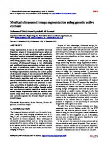
Fig. 1. (a) Synthetic texture image, (b) Magnified view of 21 × 21 window cropped around point P , shown in Fig. 1(a); (c) Mean texture feature image of Fig. 1(a). 4

5 4 3 2 1

x 10

D1 4

5 4 3 2 1

250

x 10

20

40

60

80

100

120

140

160

180

200

220

90

100

110

45

50

55

D2

200 4

5 4 3 2 1

150

x 10

50

x 10

0

50

100

150

200

250

300

350

(a)

400

450

5 4 3 2 1

30

40

50

60

70

80

5

10

15

20

25

30

35

40

D4 4

0

20

D3 4

5 4 3 2 1

100

10

x 10

5

10

15

20

25

A4 5

10

15

20

25

(b)

Fig. 2. (a) 1-D texture profile of Fig. 1(b); (b) Scalogram of the texture profile.

2.2

Discrete Wavelet transform (DWT) and scalogram

DWT analyses a signal based on its content in different frequency ranges. Therefore, it is very useful in analyzing repetitive patterns such as texture. DWT decomposes a signal into different bands (approximation and detail) with different resolution in frequency and spatial extent. Let ξ(x) be the image signal and ψu,s (x) be a wavelet function at a particular scale, then signal filtered at point u is obtained by taking the inner product of the two < ξ(x), ψu,s (x) >. This inner product is called wavelet coefficient of ξ(x) at position u and scale s [9]. Scalogram [3] of a signal ξ(x) is the variance of this wavelet coefficient: w(u, s) = E{| < ξ(x), ψu,s (x) > |2 }

(4)

The w(u, s) has been approximated by convolving the square modulus of the filtered outputs with a Gaussian envelop of a suitable width [3]. The w(u, s) gives the energy accumulated in a band with frequency bandwidth and center frequency inversely proportional to scale. We use scalogram based discrete wavelet features to model the texture characteristics of the image in our work.

3

Texture Feature Extraction

In this section, we explain how DWT is used to extract texture features of the input image. It discusses the computational framework based on multi-channel processing. We use DWT-based dyadic decomposition of the signal to obtain

texture properties. A simulated texture image shown in Fig. 1(a) is used to illustrate the computational framework with the results of intermediate processing. Modeling of texture features at a point in an image involves two steps: scalogram estimation and texture feature estimation. To obtain texture features at a particular point (pixel) in an image, a n × n window is considered around the point of interest (see Fig. 1(b)). Intensities of the pixels in this window are arranged in the form of a vector of length n2 whose elements are taken column wise from the n × n cropped intensity matrix. Let this intensity vector (signal) be ξ. It represents the textural pattern around the pixel and is subsequently used in the estimation of scalogram. 3.1

Scalogram estimation

1-D input signal ξ, obtained after arranging the pixels of n × n window as explained above, is used for the scalogram estimation. Signal ξ is decomposed using wavelet filter. We use orthogonal Daubechies 2-channel (with dyadic decomposition) wavelet filter. Daubechies filter with level-L dyadic decomposition, yields wavelet coefficients {AL , DL , DL−1 , .., D1 } where, AL represents approximation coefficient and Di ’s are detail coefficients. The steps of processing to obtain scalogram from the wavelet coefficients are described in [10]. Fig. 2(b) presents an example of scalogram obtained for the signal shown in Fig. 2(a) using level-4 DWT decomposition. 3.2

Texture Feature Estimation

Once the scalogram of the texture profile is obtained, it is used for texture feature estimation. Texture features are estimated from the “energy measure” of the wavelet coefficients of the scalogram subbands. This texture feature is similar to the “texture energy measure” proposed by Laws [11]. Let E be the texture energy image for the input texture image I. E defines a functional mapping from 2-D pixel coordinate space to multi-dimensional energy space Γ , i.e. E : [0, m] × [0, n] → Γ . Let for the k th pixel in I, Dk be the set of all subbands of scalogram S and Ek ∈ Γ be the texture energy vector associated with it. Texture energy space, Γ , can be created by taking the l1 norm of each subband of the scalogram S. Then, Γ represents L + 1 dimensional energy space for level-L decomposition of the texture signal. Formally, ith element of the energy vector Ek belonging to Γ , is given as follows:     X 1 E(k,i) = (5) S(i,j)  N j

where, i represents a scalogram subband of set Dk , S(i,j) is the j th element of the ith subband of scalogram S and N is the cardinality of the ith subband. Texture energy image computed using Eqn. 5 is a multi-dimensional image and provides good discriminative information to estimate the texture boundaries.

These texture energy measures constitute a texture feature image. Fig. 1(c) shows an image obtained by taking the mean of all bands of a texture energy image computed using Eqn. 5 for the texture image shown in Fig. 1(a). One common problem in texture segmentation is the problem of precise detection of the boundary efficiently. A pixel near the texture boundary has neighboring pixels belonging to different textures. In addition, a textured image may contain a non-homogeneous, non-regular texture regions. This would cause the obtained energy measure to deviate from “expected” values. Hence, it is necessary that the obtained feature image be further processed to remove noise and outliers. To do so, we apply smoothing operation to the texture energy image in every band separately. In our smoothing method, the energy measure of the k th pixel in a particular band is replaced by the average of a block of energy measures centered at pixel k in that band. In addition, in order to reduce the block effects and to reject outliers, the p percentage of the largest and the smallest energy values with in the window block are excluded from the calculation. Thus, the smooth texture feature value of pixel k in ith band of the feature image is obtained as:

F(k,i)

 2  (w )(1−2×p%)  X 1 = 2 E(k,j)  w (1 − 2 × p%)  j=1

(6)

where, E(k,j) s are the energy measures within the w × w window centered at pixel k of ith band of the texture energy image. The window size w × w and the value of p are chosen experimentally to be 10 × 10 and 10 respectively in our experiments. Texture feature image F , computed by smoothing the texture energy image E as explain above, is used in the computation of texture edges using inverse edge indicator function which is described in the next section.

4

Geodesic Active Contours for Texture Feature Space

We use GAC technique in the scalogram based wavelet texture feature space by using the generalized inverse edge detector function g proposed in [5]. GAC, in presence of texture feature based inverse edge detector g, is attracted towards texture boundary. Let X : Σ → M be an embedding of Σ in M , where M is a Riemannian manifold with known metrics, and Σ is another Riemannian manifold with unknown metric. As proposed in [7], metric on Σ can be constructed using the knowledge of the metric on M using the pullback mechanism [4]. If Σ is a 2-D image manifold embedded in n-dimensional manifold of texture feature space → − F = (F 1 (x, y), ..., F n (x, y)), metric h(x, y) of 2-D image manifold can be obtained from the embedding texture feature space as follows [7]: µ h(x, y) =

1 + Σi (Fxi )2 Σi Fxi Fyi Σi Fxi Fyi 1 + Σi (Fyi )2

¶ (7)

(a)

(b)

(c)

Fig. 3. Results on synthetic images: (a) Input images with initial contour, (b) Texture edge maps, (c) Segmentation results.

Then, stopping function g used in GAC model for texture boundary detection can be given as the inverse of the determinant of metric h as follows [5]: g(∇I(x, y)) =

1 1 = 2 1 + |∇I(x, y)| det(h(x, y))

(8)

where, det(h) is the determinant of h. Eqn. 3, with g obtained in Eqn. 8, is used for the segmentation of the textured object from the texture background. 4.1

Segmenting multiple textured objects

As GAC model is topology independent and does not require any special strategy to handle multiple objects, proposed method can segment multiple textured objects simultaneously. Evolving contours naturally split and merge allowing the simultaneous detection of several textured objects so number of objects to be segmented in the scene are not required to be known prior in the image. Section 5 presents some multiple textured objects segmentation results for the synthetic and natural images.

5

Experimental Results

We have used our proposed method on both synthetic and natural texture images to show its efficiency. For an input image, texture feature space is created using the DWT and scalogram, and Eqn. 5 is used for texture energy estimation. We use the orthogonal Daubechies 2-channel (with dyadic decomposition) wavelet filter for signal decomposition. The metric of the image manifold is computed considering the image manifold embedded in the higher dimensional texture feature space. This metric is used to obtain the texture edge detector function of GAC. Initialization of the geodesic snake is done using a signed distance function. To start the segmentation, an initial contour is put around the object(s) to be segmented. Contour moves towards the object boundary to minimize objective function LR (Eqn. 1) in the presence of new g (Eqn. 8). Segmentation results obtained using proposed technique are shown in Fig. 3 and Fig. 4 for synthetic and natural images respectively. Input texture images are shown with the initial contour (Fig. 3(a) and Fig. 4(a)). Edge maps of the input synthetic and natural

texture images, computed using Eqn. 8, are shown in Fig. 3(b) and Fig. 4(b) respectively. Final segmentation results are shown in Fig. 3(c) and Fig. 4(c). Results obtained are quite encouraging and promising. Fig. 5 shows comparative results for zebra example. We can carefully observe that our result is superior than the results of other techniques. The results reported in the literature show errors in any one of the following places of the object (mouth, back, area near legs etc.). The overall computation cost (which includes the cost of texture feature extraction and segmentation) of the proposed method lies in the range of 70 to 90 seconds on a P-IV, 3 GHz machine with 2 GB RAM for images of size 100 × 100 pixels.

(a)

(b)

(c)

Fig. 4. Results on natural images: (a) Input images with initial contour, (b) Texture edge maps, (c) Segmentation results.

6

Conclusion

In this paper, we present a technique for multiple textured objects segmentation in the presence of background texture. The proposed technique is based on GAC

and can segment multiple textured objects from the textured background. We use DWT and scalogram to model the texture features. Our main contribution in this work lie in the development of new DWT and scalogram based texture features which have a strong discriminating power to define a good texture edge metric to be used in GAC. We validated our technique using various synthetic and natural texture images. Results obtained are quite encouraging and accurate for both types of images.

(a)

(b)

(c)

(d)

Fig. 5. Comparative study of results: (a) reproduced from [12], (b) reproduced from [13], (c) obtained using the method presented in [14], (d) proposed technique.

References 1. Caselles, V., Kimmel, R., Saprio, G.: Geodesic active contours. Int. J. of Computer Vision 22(1) (1997) 61–79 2. Sapiro, G.: Color snake. CVIU 68(2) (1997) 247–253 3. Clerc, M., Mallat, S.: The texture gradient equations for recovering shape from texture. IEEE Trans. on PAMI 24(4) (2002) 536–549 4. Sochen, N., Kimmel, R., Malladi, R.: A general framework for low level vision. IEEE Trans. on Image Proc. 7(3) (1998) 310–318 5. Sagiv, C., Sochen, N.A., Zeevi, Y.Y.: Gabor-space geodesic active contours. LNCS 1888 (2000) 309–318 6. Paragios, N., Deriche, R.: Geodesic active regions for supervised texture segmentation. In: Proc. of ICCV’ 99. (1999) 926–932 7. Sagiv, C., Sochen, N., Zeevi, Y.: Integrated active contours for texture segmentation. IEEE Trans. on Image Proc. 15(6) (2006) 1633–1646 8. Kass, M., Witkin, A., Terzopoulos, D.: Snakes: Active contour models. Int. J. of Computer Vision 1(4) (1988) 321–331 9. Mallat, S.: A Wavelet Tour of Signal Processing. Academic Press (1999) 10. Surya Prakash, Das, S.: External force modeling of snake using DWT for texture object segmentation. In: Proc. of ICAPR’ 07, ISI Calcutta, India (2007) 215–219 11. Laws, K.: Textured image segmentation. PhD thesis, Dept. of Elec. Engg., Univ. of Southern California (1980) 12. Rousson, M., Brox, T., Deriche, R.: Active unsupervised texture segmentation on a diffusion based feature space. In: Proc. of CVPR’ 03. (2003) II–699–704 13. Awate, S.P., Tasdizen, T., Whitaker, R.T.: Unsupervised texture segmentation with nonparametric neighborhood statistics. In: Proc. of ECCV’ 06. LNCS 3952 (2006) 494–507 14. Gupta, L., Das, S.: Texture edge detection using multi-resolution features and self-organizing map. Proc. of ICPR’ 06 (2006)