Abstract: - This paper presents MATLAB programs for generating the coefficients of the lowpass analysis filter corresponding to orthonormal wavelet analyses.
MATLAB Programs for Generating Orthonormal Wavelets B.G. SHERLOCK and Y.P. KAKAD Department of Electrical and Computer Engineering University of North Carolina at Charlotte Charlotte, NC 28223 USA
Abstract: - This paper presents MATLAB programs for generating the coefficients of the lowpass analysis filter corresponding to orthonormal wavelet analyses. One of the programs generates the famous Daubechies maxflat wavelets, and a second generates the Daubechies complex symmetric orthonormal wavelets. The remaining two programs generate the space of all orthonormal wavelets in terms of parameterizations whereby the space of wavelets of a given length 2N is generated by N parameters. This software should prove useful where it is desired to perform an optimization to obtain the best wavelet for a given application. Key-Words: - Wavelets, Orthonormal, Software, Parameterization
1 Introduction Wavelet analysis has been widely used in recent years in a variety of application areas. The reason for this success is that wavelet analysis provides a mixed time-frequency representation that gives a useful compromise between analysis purely in terms of frequency (as exemplified by the Fourier transform) and purely time-domain analysis. A further advantage is that, unlike the Discrete Fourier Transform, the Discrete Wavelet Transform (DWT) is not unique – the user may choose between an infinite number of different wavelets, each providing its own unique corresponding DWT. This opens up the possibility of performing an optimization procedure in order to obtain the “best” wavelet for any given application according to some given optimality criterion. In order to perform this optimization, it is necessary to have a parameterization of the space of wavelets under consideration. The optimization cost function will then be passed the values of the parameters for each wavelet as the optimization proceeds. One of the authors has successfully used this approach to obtain optimal wavelets for the compression of fingerprint images [7]. The main disadvantage of orthonormal wavelet analysis is that symmetry of real-valued filters cannot be achieved. Symmetry is of great importance because of the linear phase exhibited by such filters, and also because symmetry permits the use of a reflective data extension that substantially reduces edge effects. The usual way of obtaining linear phase filters within the context of a wavelet analysis is to relax the requirement of orthonormality, and this has led to the widespread use of biorthogonal wavelets [1]. Linear phase is
obtained at a cost, however: the DWT using biorthogonal wavelets does not preserve energy, i.e. the Parseval relation is no longer valid. It is possible to obtain linear phase without sacrificing orthonormality if we allow the coefficients of the filter to be complex. In the paper we show how the parameterizations can be used to generate spaces of symmetric orthonormal wavelets. Two further MATLAB programs are included. One of these generates the lowpass filter coefficients for the famous Daubechies maxflat wavelets, and the other for the Daubechies maxflat symmetric complex wavelets.
2 The Space of Orthonormal Wavelets In this section, software is presented to generate the coefficients for the scaling filters corresponding to all orthonormal wavelets, including wavelets with complex filter coefficients. To do this, a parameterization of the space of orthonormal wavelets is required. We make use of two parameterizations; each of these generates scaling filter coefficents from a given set of parameter values. To generate the space of all orthonormal wavelets with real-valued coefficients, the parameterization of Section 2.1 requires the parameters to be angles in the range 0 to 2π, whereas that of Section 2.2 allows the parameters to have any real values. Both parameterizations produce the space of orthonormal wavelets with complex coefficients if the parameters are given complex values. The major advantage of complex orthonormal wavelets over real orthonormal wavelets is that linear phase can be achieved.
2.1 Generating Parameters
Wavelets
Using
Angle
Let the coefficients of the scaling filter be denoted by {hi }, with z-transform H ( z ) = hi z − i .
∑ i
Vaidyanathan [9] proposed the following parameterization of the space of all perfectreconstruction two-channel filter banks of length 2M in terms of M angle parameters {θ 0 , θ 1 ,..., θ M −1 }:
M −1 1 H ( z ) = (1 0)R0 ∏ ΛRi −1 , where i =1 z si ci 1 0 , with Λ = and R i = −1 0 z − si ci c i = cos θ i and s i = sin θ i . Sherlock and Monro [6] derived from this recursive formulae expressing the coefficients
{h } for a filter of length 2(k+1) in terms of the coefficients {h } for a filter of length 2k. They ( k +1) i
(k ) i
obtained, for the even numbered filter coefficients {h2i } :
h0( k +1) = ck h0( k ) ( k +1) (k ) (k ) h2 i = ck h2 i − sk h2 i −1 for i = 1, 2, ..., k − 1 ( k +1) (k ) h2 k = − sk h2 k −1 with h0(1) = c0 and h1(1) = s0 . The corresponding formula for the odd numbered filter coefficients {h2i +1} is:
h1( k +1) = s k h0( k ) ( k +1) (k ) (k ) h2i +1 = s k h2i + c k h2i −1 for i = 1, 2, ..., k − 1 h ( k +1) = c h ( k ) k 2 k −1 2 k +1 The recurrence of the above equations can be elegantly expressed in the form of the flow diagram of Figure 1. In this diagram a filter of any desired
even length 2M can be produced by choosing M parameters θ i (with
∑θ i
i
=
π if regularity is 4
desired) and passing through the flow diagram, terminating after M-1 stages of processing. An efficient implementation in MATLAB is given in Figure 2. function h = orthogen(alpha); % Constructs an array, h(1...N) of lowpass % orthonormal FIR filter coefficients for any % even N>=2. The input array, alpha(1...N/2) % gives N/2 free parameters that are angles % in radians. If the angles sum to pi/4 the % filter corresponds to a regular wavelet. N = 2*length(alpha); h = zeros(1, N); lo = N/2; hi = lo + 1; h(lo) = cos(alpha(1)); h(hi) = sin(alpha(1)); nstages = N/2; for stage = 1 : nstages-1 c = cos(alpha(stage+1)); s = sin(alpha(stage+1)); h(lo-1) = c*h(lo); h(lo) = s*h(lo); h(hi+1) = c*h(hi); h(hi) = -s*h(hi); nbutterflies = stage-1; butterflybase = lo+1; for butterfly = 1 : nbutterflies hlo = h(butterflybase); hhi = h(butterflybase+1); h(butterflybase) = c*hhi - s*hlo; h(butterflybase+1)= s*hhi + c*hlo; butterflybase = butterflybase + 2; end; lo = lo - 1; hi = hi + 1; end;
Figure 2. MATLAB function for generating orthonormal wavelets from angle parameters.
This parameterization is, however, a redundant representation because of inherent symmetries in our parameter space. It is shown in [6] that the filter coefficients will be unchanged if any even number of the θ i are changed by π. The space can therefore be fully covered by choosing θ 0 from the interval [0,2π) and θ 1 through θ M −1 from [0,π). When generating wavelets, however, regularity, M −1
equivalent to
∑θ i =0
i
=
π , is also required. With this 4
additional constraint, it is shown in [6] that the space of all orthonormal wavelets of length 2M is covered by choosing M-1 parameters θ i from the interval
Figure 1. Flow diagram illustrating generation of orthonormal wavelets from angle parameters.
[0,π), and calculating the final one from the regularity constraint. For a filter of length 2M corresponding to an orthonormal wavelet, the transformation
π −θ 0 , 2 θ i′ = π − θ i , i = 1,2,..., M − 2 θ 0′ =
transforms the filter into its time-reverse. Therefore, half of the parameter space corresponds to wavelets which are time-reversals of the other half. A subspace of the parameter space which covers all orthonormal wavelets but excludes their time reversals is given (for length-2M wavelets) by choosing one parameter from the interval [0,π/2), M2 parameters [0,π), and calculating the remaining parameter from the regularity constraint. The parameterization can be extended to produce filters with complex-valued coefficients, simply by allowing the θ i to be complex. However, the parameterization of Section 2.2 turns out to be better suited to this purpose.
2.2 Generating Wavelets Using Real-Valued Parameters The parameterization used in this section is based upon the work of Pollen [5] and the subsequent results of Lina [3,4]. As in Section 2.1, let the coefficients of the scaling filter be denoted by {hi }, with z-transform H ( z ) =
∑h z i
−i
.
Then the
i
parameterization of the space of all regular perfectreconstruction two-channel filter banks of length 2M+2 in terms of M parameters {ν 0 ,ν 1 ,...,ν M −1 } is produced as described below. Define 2-by-2 matrices G i (z ) by
u i ( z ) wi ( z ) Gi ( z) = , i=0,…,M-1. − w ( z) u ( z) i i ν iν i ( z −1 − 1) where u i ( z ) = 1 + 1 + ν iν i νi and wi ( z ) = ( z − 1) . 1 + ν iν i Then form G ( z ) = G 0 G1T G 2 G 3T ...G M − 2 G MT −1 , where the notation G T represents the conjugate transpose. Note that conjugate transposition is applied to every second matrix in the above product. Finally, the filter coefficients in this parametrization are obtained as
H ( z) =
1 2
(1
z − 1)G ( z 2 ) . − 1
Because, just as in Section 2.1, the filter is produced by a successive product of matrices, it is
also possible to express the present parameterization in the form of a recurrence. Lina and Mayrand [3] presented recursive formulae expressing the coefficients hi( k +1) for a filter of length 2(k+1) in
{
}
{ } for a filter of length
terms of the coefficients hi( k )
2k. They obtained, for the even numbered filter coefficients {h2 i } : h2( ik +1) =
(
)
1 h2(ik ) − ν k h2(ik−)1 + ν k h2(ik+)1 + ν kν k h2(ik−)2 ( −1) k , 1 + ν kν k
and for the odd numbered filter coefficients {h2i +1} : h2( ik++11) =
(
)
1 h2(ik+)1 − ν k h2(ik ) + ν k h2(ik+)2 + ν kν k h2(ik+)1+ 2 ( −1) k . 1 + ν kν k
The recurrence is started with the Haar length-2 wavelet, h0(1) = h1(1) = 12 ; then regularity of the wavelet is preserved throughout the iterative process irrespective of the choice of ν i . An advantage over the parameterization in Section 2.1 is that this parameterization does not exhibit the redundancies that occurred in Section 2.1 due to the angular nature of the θ i parameters. Here, the space of all orthonormal regular wavelets with real coefficients is simply produced by allowing the ν i to range over all real values. Furthermore, restricting all ν i to be pure imaginary generates the space of all symmetric complex orthonormal wavelets. These wavelets are important because they are the only orthonormal function h=nuorthgen(nus) % Generates all orthonormal regular wavelets. % nus is an array of parameters satisfying: % nus all real => space of all real % orthonormal regular wavelets % nus all imaginary => space of all % symmetric complex orthonormal % regular wavelets % nus complex => space of all orthonormal % regular wavelets h0 = 1/sqrt(2); h1 = 1/sqrt(2); h=[h0 h1] ; stages=length(nus); for stage=1:stages nu=nus(stage); nuc=conj(nu); N=length(h)+2; h=[0 0 conj(h) 0 0]; for i=2:2:N+1 newh(i)= h(i)-nu*h(i-1)+nu*h(i+1)+ ... nu*nuc*h(i+2); i1=i+1; newh(i1)=h(i1)-nuc*h(i1-1)+ ... nuc*h(i1+1)+ nu*nuc*h(i1-2); end h=newh(2:N+1)/(1+nu*nuc); end
Figure 3. MATLAB function for generating orthonormal wavelets using parameterization of Section 2.2.
wavelets that exhibit linear phase. Linear phase is highly valuable in many applications because the position of details is preserved in the filtered signal. An efficient implementation in MATLAB is given in Figure 3.
3 Daubechies Wavelets 3.1 Generating Wavelets
Daubechies
Maxflat
The Daubechies maxflat wavelet of length 2N is the unique length 2N wavelet whose frequency response has both minimum phase and also exhibits N zero derivatives at ω = 0 [2]. These wavelets are widely used because of their regularity. The wavelet is obtained by a spectral factorization of the following halfband frequency response [8]: N
1 + cos ω N −1 N + k − 1 1 − cos ω P (ω ) = 2 ∑ k 2 2 k =0 1 − cos ω Introduce y = ; then y , ω , and the z2 transform
variable
are
related
by
−1
z+z cos ω = = 1 − 2 y . Expressing P(ω ) in 2 ~ terms of y yields P ( y ) = 2(1 − y ) N B N ( y ) , where N −1 N + k − 1 k B N ( y ) = ∑ y is the binomial series k k =0
truncated after N terms. The spectral factorization of P (ω ) and the subsequent determination of the scaling filter coefficients are performed as follows: 1. Find the N-1 zeros {y i } of the polynomial
BN ( y) . 2. Transform these to the z domain using
z i = 1 − 2 y i ± (1 − 2 y i ) 2 − 1 . Because of the square root, this yields a total of 2N-2 values. 3. Of the 2N-2 values of z i , retain only those N-1 that have
z i < 1 . This choice results in a
minimum phase filter. 4. Include a further N zeros at z = −1 . The coefficients of the resultant polynomial are the taps of the scaling filter for the Daubechies maxflat filter of length 2N. This procedure is implemented in the MATLAB program of Figure 4, which generates these wavelets.
k
function dau=makedau(N) % Function to generate coefficients of % Daubechies maxflat orthonormal wavelet % filter of length N. % if mod(N,2) ~=0 error('N must be even'); end p=N/2; b(p)=1; for i=p-1:-1:1 b(i)= b(i+1)*(2*p-i-1)/(4*(p-i)); end r=roots(b)/4; z1= (1-2*r) + sqrt((1-2*r).^2 -1); z2= (1-2*r) - sqrt((1-2*r).^2 -1); z=[z1;z2]; zchoose = z( abs(z) 1 and positive real 4 part. What this does is to reduce each quadruplet
( zi , zi−1 , zi , zi−1 ) of roots to a single root outside the unit circle and having positive imaginary part. 3b. Sort these
N −1 roots into increasing order of 2
real part. 3c. Distribute these
N −1 roots evenly above and 2
below the real axis, by taking the conjugate of every second root. 3d. Include the inverse of each root. This results in a total of N-1 roots. Note that for step 3a to succeed, it is necessary that
2N − 2 be an integer, i.e. that N be odd. 4
Consequently, symmetric complex Daubechies wavelets exist only for odd N, i.e. filters of length 2N = 2, 6, 10, 14, etc. A MATLAB function to generate these wavelets is presented in Figure 5. function dau=makecxdau(N) % Function to generate coefficients of % Daubechies maxflat symmetric complex % orthonormal wavelet filters. % if mod(N,2) ~=0 error('N must be even'); end p=N/2; b(p)=1; for i=p-1:-1:1 b(i)= b(i+1)*(2*p-i-1)/(4*(p-i)); end r=roots(b)/4; z1= (1-2*r) + sqrt((1-2*r).^2 -1); z2= (1-2*r) - sqrt((1-2*r).^2 -1); z=[z1;z2]; % Keep one of every quadruplet z, 1/z, zbar, % 1/zbar: zchoose = z( abs(z)>1 & imag(z) >0); % sort in order of increasing real part: [junk,index]= sort(real(zchoose)); zchoose = zchoose(index); % Distribute evenly above / below real axis: zchoose(1:2:length(zchoose))=... conj(zchoose(1:2:length(zchoose))); zchoose = [zchoose; 1./zchoose]; if(length(zchoose) ~= length(z)/2) disp('No symmetric solutions for this N:') error('N must be of form 2*(odd number)') end q=poly(zchoose); % add p zeros at -1 flat=1; for i=1:p flat=conv(flat,[1 1]); end dau= conv(q,flat); dau= sqrt(2)*dau/sum(dau);
Figure 5. MATLAB function for generating complex symmetric Daubechies maxflat wavelets.
4 Conclusion We have presented MATLAB implementations of two parameterizations of the space of orthonormal wavelets. In addition to their obvious use in generating wavelets with real coefficients, we have indicated how these may be used to generate symmetric wavelets with complex coefficients. This software would be useful in an optimization task in which the “best” wavelet for a given application is sought. We also presented MATLAB functions that produce the commonly encountered Daubechies max-flat wavelets, as well as the symmetric complex Daubechies wavelets. References: [1] A. Cohen, I. Daubechies and J.C. Feauveau, Biorthogonal bases of compactly supported wavelets, Comm. Pure Appl. Math., vol. 45, 1992, pp 485-560. [2] I. Daubechies, Orthonormal bases of compactly supported wavelets, Comm. Pure Appl. Math., vol. 41, 1988, pp 909-966. [3] J.M. Lina and M. Mayrand, Complex Daubechies Wavelets, University of Montreal Laboratory of Nuclear Physics Report UdeMPHYSNUM-ANS-15, December 1993. [4] J.M. Lina and M. Mayrand, Parameterizations for Daubechies Wavelets, Physical Review E, Vol. 48, No. 6, 1993, pp. R4160-R4163. [5] D. Pollen, SU1(2,F(z,1/z)) for F a subfield of C, Journal of the American Mathematical Society, Vol.3, No.3, 1990, pp. 611-624. [6] B.G. Sherlock and D.M. Monro, On the Space of Orthonormal Wavelets, IEEE Transactions on Signal Processing, Vol. 46, No. 6, 1998, pp. 1716-1720. [7] B.G. Sherlock and D.M. Monro, Optimized Wavelets for Fingerprint Compression, IEEE International Conference on Acoustics, Speech and Signal Processing (ICASSP-96), Atlanta, Georgia, May 1996, Vol. III, pp. 1447-1450 [8] G. Strang and T. Nguyen, Wavelets and Filter Banks, Wellesley-Cambridge Press, 1996. [9] P.P. Vaidyanathan, Multirate Systems and Filter Banks, Prentice Hall, 1992.