Generating Optimized Decision Tree Based on

Kiran Kumar Reddi et al. / International Journal of Engineering Science and Technology Vol. 2(3), 2010, 157-164

Generating Optimized Decision Tree Based on Discrete Wavelet Transform Kiran Kumar Reddi*1 Ali Mirza Mahmood2 K.Mrithyumjaya Rao3

1. Assistant Professor, Department of Computer Science, Krishna University, Machilipatnam, India 2. Assistant Professor, Department of Computer Science, DMSSVH College of Engineering, Machilipatnam, India 3. Professor, Department of Computer Science & Engineering, Vaagdevi College of Engineering. *Corresponding Author E-mail address:[email protected] Abstract: Increasing growth of functionality in current IT trends proved the decision making operations through mass data mining techniques. There is still a requirement for further efficiency and optimization. The problem of constructing the optimization decision tree is now an active research area. Generating an efficient and optimized decision tree with multi-attribute data source is considered as one of the shortcomings. This paper emphasizes to propose a multivariate statistical method Discrete Wavelet Transform on multi-attribute data for reducing dimensionality and to transform traditional decision tree algorithm to form a new algorithmic model. The experimental results described that this method can not only optimizes the structure of the decision tree, but also improves the problems existing in pruning and to mine the better rule set without effecting the purpose of prediction accuracy altogether. Keywords: Optimized decision tree. Multivariate Statistical Method. Discrete Wavelet Transform. Haar Wavelet.

I. Introduction The classification is an important part of data mining technique in research application field. There are different types of classification models such as decision trees, SVM, neural networks, Bayesian belief networks, Genetic algorithm etc.. These above mentioned methods have provided satisfactory results, but still the most widely used classification models is the decision trees. Because of the simple structure, the wide applicability on real time problems, the high efficiency and the high accuracy. The most common methods for creating decision trees are from data and rule, popularly known as Data based decision tree and Rule-based decision tree respectively [Amany (2009)].Decision tree induction is one of the most important branch of inductive learning, and it is one of the most widely used and practical method for inductive inference .Decision tree is induced by Quinlan for inducing classification models [Quinlan J R. (1986)]. In decision tree induction the entire data in the training set is used as root node for the tree. Then the root node is split into several sub-nodes depending upon some heuristic function. Splitting of sub-node continues, till all leaf nodes are generated else if all the instances in the sub-node belong to the same class. The different variation of decision trees can be generated depending upon two main parameters, one is heuristic function used and the other is pruning method involved. The heuristic function used can be the Gini index, the entropy, the information gain, the gain ratio and recently the large margin heuristic [Ning Li. 2009] is proposed by Ning li. The most commonly used decision tree algorithms are ID3 [2] and C4.5 [Quinlan J R.(1993) ]. In ID3 the heuristic function used for splitting the data is Information Gain, which is the quality of information gained by partitioning the set of instances. The defect of this heuristic function is it has a strong bias in favor of the attributes with many outcomes. To solve this problem C4.5 uses another heuristic function, which penalizes the attribute that produces a wider distribution of data. This measure is commonly known as Gain Ratio. Pruning is one of the most successful methods used in decision tree construction. The original work in pruning is proposed to tolerate noise in the training data [L. Breiman, 1984] [Quinlan J R. (1987)].In

ISSN: 0975-5462

157

Kiran Kumar Reddi et al. / International Journal of Engineering Science and Technology Vol. 2(3), 2010, 157-164 [Floriana Esposito (1997) ], [L.A. Breslow, (1997) ], [Wang Xizhao (2004) ], the authors made through comparison of various pruning methods. Two broad classes of methods are proposed for pruning. Pre-pruning: Stop growing the tree earlier based on some stopping criteria, before it classifies the training set perfectly. One of the simplest method is setting a threshold for each sample when arriving the node; other method is to calculate the impact of system performance on each expansion and it is restricted if the gain is less than the threshold. In pre-pruning, the advantage is not generating full tree, disadvantage is horizon effect phenomenon [Quinlan J R.(1993) ]. Post-pruning: It has two major stages: Fitting and Simplification. First of all, it allows over-fitting the data, and then post-prunes the grown tree. In practice post-pruning methods has a better performance than pre-pruning. A lot of methods are presented based on different heuristics, in [L Breiman, J. H. Friedman (1984)], the author proposed Minimal Cost Complexity Pruning (MCCP), Pessimistic Error Pruning (PEP), is proposed by J.R.Quinlan which uses continuity correction for the binomial distribution to provide a more realistic error rate instead of the optimistic of error rate in training set. In [Quinlan J R.(1993) ], the author proposed Error Based Pruning (EBP) which uses prediction of error rate (a revised version of PEP).In [Quinlan J R.(1987) ], the author proposed Reduced Error Pruning (REP), which finds the smallest version of the most accurate sub-tree but it tends to over-prune the tree. Recently in [Jin-Mao(2009) ], the author proposed Cost and Structural complexity (CSC) pruning, which takes into account both classification accuracy and structural complexity. Post-pruning can be further divided into two categories. One exploit the training set alone, other withhold a part of the training set for validation. Pessimistic Error Pruning (PEP), Error Based Pruning (EBP), comes under first category and Minimum Error Pruning (MEP), Critical value Pruning (CVP) comes under second. II. Related Work Considering the problem in decision tree optimization a novel approach of decision tree construction is presented based on discrete wavelet transform analysis. In order to construct the optimized decision tree and remove the pruning, noise and abnormal data should be filtered while generating decision tree. A. Wavelet Transform: The Discrete Wavelet Transform (DWT) is a linear signal processing technique that, when applied to a data vector X, transforms it to a numerically different vector X’, of wavelet coefficient. The discrete wavelet transform uses the idea of dimensionality reduction, which is a multivariate statistical method that stores the compressed approximation of the data under the premise of little loss of information. A compressed approximation of the data can be retained by storing only a small fraction of the user-specified threshold wavelet coefficients and remaining data as zero. This technique also works well to remove noise and abnormal data without smoothing out the main features of data [Jiawei Han (2006)].DWT algorithmic complexity for an input vector of length n is O(n). Discrete wavelet transform can be better applicable at handling data of high dimensionality. B. Haar Wavelet Transform: A Haar wavelet transform is the simplest type of wavelet [James S. Walker.(1999) ].In discrete form, Haar wavelet transform are related to a mathematical operation called the Haar Transform. The Haar transform serves as a prototype for all other wavelet transforms. A Haar transform decomposes an array into two halves of the original length of the array. One half is a running average, and the other half is a running difference. Haar transform performs an average and difference on a pair of values. Procedure: To Calculate the Haar transform of an array of n samples: 1. Find the average of each pair of samples. (n/2 averages) 2. Find the differences between each average and the sample it was calculated from. (n/2 differences)

ISSN: 0975-5462

158

Kiran Kumar Reddi et al. / International Journal of Engineering Science and Technology Vol. 2(3), 2010, 157-164 3. Fill the first half of the array with averages. 4. Fill the second half of the array with differences. 5. Repeat the process on the first half of the array. Array= [average/difference] For example, Array [9, 7, 3, 5], Elements 4 2 1

Average [9,7,3,5] [8,4] [6]

Coefficient [1,-1] [2]

So, Haar Transform array is [6, 2, 1,-1] The Haar wavelet transform has a number of Advantages: • It is conceptually simple. • It is fast. • It is memory efficient, since it can be calculated in place without a temporary Array. • It is exactly reversible without the edge effects that are a problem with other Wavelet transforms. III. Building the Decision Tree Based on Haar Wavelet Transform Step 1: Convert data source into a multi-matrix, Identify the main attributes by Haar wavelet transform. 

Data matrix conversion

x11x12...x1n  x21x22...x2n   x  x1, x2,...xn  ....................  1   .....................  xp1xp2...xpn Where p is object’s attribute and n is the attributes value 

Calculate the average and Difference

a

l  r  2

d  ar ra

2 3

Where a, d, l, r are average, difference, left and right elements respectively. Step 2: Do data cleaning for data source and generate the training set of decision tree through the converting of continuous data into discrete variable. Step 3: Compute the information (entropy) of training sample sets, the information (entropy) of each attribute, split information, split gain and information gain ratio, of which S stands for training sample sets and A denotes the attributes.  Compute the Information(Entropy) of training sample set S,

ISSN: 0975-5462

159

Kiran Kumar Reddi et al. / International Journal of Engineering Science and Technology Vol. 2(3), 2010, 157-164 m

IS    Pi log2Pi i 1

Where Pi is the probability of Category Ci in S. 

Compute the information(Entropy) of the attribute A, m

Si ES , A   I S , A i 1 S 

Compute information gain of A

GainS , A  I S   E S , A 

Compute split information of A m

Split_ InfoS, A  

Si

i 1



S

log2

Si S

Computer information gain ratio of A

Gain _ Ratio S , A  

Gain S , A  I S , A 

for continuous attribute values, calculate information gain ratio corresponding with the segmentation points divided by ai (i = 1, 2,3,… , n−1) and choose the maximum rate of information gain ai as the split points of attribute classification. Choose the maximum attribute of information gain as the decision tree root. Step 4: Each possible value of root may correspond to a subset. Do step 3 recursively and generate decision tree for the sample subset until the observed data of each divided subset are the same in the classification attributes. Step 5: Extract the classification rules based on the constructed decision tree and do classification for new data sets. IV. Case Study and Comparative Analysis A. The Improved decision tree algorithm example: The details of the Pima_indiana diabetes data set is shown in Table 1. There are eight conditional attributes and one class attribute. A total of 768 instances are there in the dataset. Table 1. The pima_indiana diabetes dataset.

Case Preg Plas Pres Skin 1 6 148 72 35 2 1 85 66 29 3 8 183 64 0 ----- ----- -767 1 126 60 0 768 1 93 70 31

Insu 0 0 0 --0 0

Mass 33.6 26.6 23.3 ---30.1 30.4

Pedi Age 0.627 50 0.351 31 0.672 32 ---- -0.349 47 0.315 23

Class Posi Nega Posi --Posi Nega

Now we perform the operation of averaging and differencing to arrive at a new matrix[G. Beylkin(1991) ]. Let us look how the operation is done. Consider the first row of the converted data source into a multi-attribute matrix below,

ISSN: 0975-5462

160

Kiran Kumar Reddi et al. / International Journal of Engineering Science and Technology Vol. 2(3), 2010, 157-164

 6 148 72 35 0  1 85 66 29 0   8 183 64 0 0   --- --- -- 1 126 60 0 0   1 93 70 31 0

33.6 0.627 50  26.6 0.351 31  23.3 0.67232   -- --- - 30.1 0.349 47   30.4 0.315 23 

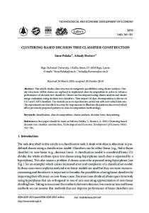
First row is, [6, 148, 72, 35, 0, 33.6, 0.627, 50] Using equation 2 , Averaging: (6+148)/2=77, (72+35)/2=53.5, (0+33.6)/2=16.8, (0.627+50)/2=25.3135. Using equation 3 , Differencing: 6–77 = –71, 72–53.5=18.5, 0–16.8 = –16.8, 0.627–25.3135 = –24.6865. So, the transformed row becomes (77, 53.5, 16.8, 25.3135, –71, 18.5, –16.8, –24.6865).Now the same operation on the average values i.e. (77, 53.5, 16.8, 25.3135) is performed. Then we perform the same operation on the averages i.e. first two elements of the new transformed row. Thus the final first transformed row becomes (41.653375, 20.596625, 11.75, –4.25675, –71, 18.5,–16.8, – 24.6865).Perform the same operation on each row of the entire matrix. Then performing the same operation on each column of the entire matrix. The final matrix which is obtained is shown in Figure 1.

  1.152178 0.290573 0.07648 - 0.108502 - 0.276321 0.167322 - 0.35408 - 0.176012     0.70694 0.22635 - 0.173977 0.056595 - 0.260436 0.175401 - 0.280314 - 0.035426    0.954234 0.399717 0.432798 - 0.04486 - 0.317498 0.370941 - 0.245538 0.049707   ------------------ ------- ------ - - - - - - - - - - - - - - - - - - -    0.77125 0.065818 0.100093 - 0.050231 - 0.406121 0.347757 - 0.317197 - 0.224591     - 0.320358 0.047986  0.707335 0.291851 - 0.180371 0.159263 - 0.288862 0.1843  

                     

Figure 1.The Final matrix.

ISSN: 0975-5462

161

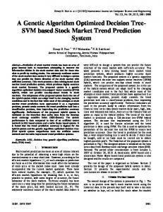
Kiran Kumar Reddi et al. / International Journal of Engineering Science and Technology Vol. 2(3), 2010, 157-164 According to step2-step4 of the decision tree algorithm in the dimensionality reduction function, the returned final decision tree is shown in Figure 2.

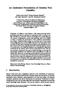
B. the Classical decision tree algorithm example: According to the data in table 1, the tree generated by the C4.5 algorithm is shown in figure 3. C. The Comparison between the Traditional Decision Tree Algorithm and Improved Algorithm example

ISSN: 0975-5462

162

Kiran Kumar Reddi et al. / International Journal of Engineering Science and Technology Vol. 2(3), 2010, 157-164 Table: 3 the comparison table of Experimental data:

Constr. Method C4.5 Improved Decision Tree

Attribute Tree number Height

Tree Size

Leaves

8

9

39

23

8

8

33

18

V. Conclusion and Future Research In This paper, A decision tree model based on Discrete Wavelet Transform was presented. We had used Haar transform as the dimensionality reduction function. The experimental results showed that this method can not only improve the efficiency when processing with massive data using the decision tree, but also optimize the structure of decision tree, improve the problem existing in pruning algorithm, and mine the better rules without affecting the purpose of prediction accuracy. Our future research work is to construct a decision tree with balance between pruning and accuracy.

Figure 2.The decision tree with dimensionality reduction function.

ISSN: 0975-5462

163

Kiran Kumar Reddi et al. / International Journal of Engineering Science and Technology Vol. 2(3), 2010, 157-164 References: [1] [2] [3] [4] [5] [6] [7] [8] [9]

Amany Abdelhalim, Issa Traore (2009) A New Method for Learning Decision Trees from Rules, Proceedings of International Conference on Machine Learning and Applications, 2009. Floriana Esposito, Donato Malerba, (1997) A comparative analysis of methods for pruning decision trees, IEEE Transcations on pattern analysis and machine intelligence, Vol 19, no 5, pp. 476-491,1997 G. Beylkin, R. Coifman, and V. Rokhlin,(1991) Fast wavelet transforms and numerical algorithms, I. Communications on Pure and Applied Mathematics, 44(2): 141-183 James S. Walker. 1999. A Primer on Wavelets and Scientific Applications. Jiawei Han, Micheline Kamber Data mining: concepts and techniques: Second Edition illustrated. Morgan Kaufmann Publishers, Inc, 2006. 5.Jin-Mao Wei,Shu Qin Wang, Gang Yu,Li Gu, Guo- Ying Wang, Xiao-Jie Yuan (2009), A Novel method for pruning decision tree, Proceedings of the Eighth International Conference on Machine Learning and Cybernetics, Baoding, 12-15 July 2009. L.A. Breslow, D.W.Aha “Simplifying decision trees: A Survey “, Knowledge engineering review, vol 12, no.1, pp 1-40, 1997. L. Breiman, J. Friedman, R. olshan, and C.Stone 1984), Classification and Regression trees, California, Wadsworth international 1984. Ning Li, Li Zhao, Ai-Xia Chen, Qing-Wu Meng, Guo-Fang Zhang(2009) A New Heuristic Of The Decision Tree Induction , Proceedings of the Eighth International Conference on Machine Learning and Cybernetics, Baoding, 12-15 July 2009. Quinlan J R.(1986) “Induction of decision tree”, Machine Learning, 1986, 1:81~106.

[10] Quinlan J R.(1993) C4.5: Programs for machine learning [M]. California: Morgan Kaufmann Publishers, Inc, 1993. [11] Quinlan J R.(1987) , Simplifying decision trees, International journal of Man-Machine studies, Vol 27,pp 221-234. [12] Wang Xizhao, You Ziying, “A Brief survey of methods for Decision tree Simplification.”Computer Engineering and Applications. Vol 40, No.27, pp.66- 69, 2004

ISSN: 0975-5462

164