Generator based Modeling CP Game for Gene Regulatory Network

Generator based Modeling CP Game for Gene Regulatory Network C. Chettaoui1 , F. Delaplace1 , P. Lescanne2 1

IBISC, FRE 2873 CNRS - Univ. Evry LIP, UMR 5668 CNRS - ENS Lyon

2

Abstract. This paper introduces a framework based on game theory that models gene regulation activities. Strategic games which are the basic model in game theory was successfully applied to gene regulation networks and molecular networks. The games used here are called Conversion/Preference games or CP Games in short. CP game theory is a discrete approach to game theory that extends nicely strategic game theory. A group of genes is a module if a connection between the regulation activity of that group of genes and some biological functions can be established. One of the main issue when a gene regulation system is analyzed through a model is to decompose the model into modules. Assuming that a gene regulation system can be decomposed into modules and that each module ”implements” a function, the goal of dynamical analysis is to exhibit the module structure. More specifically we focus on regulation equilibria that give a stable answer to stress One of the key issue in order to identify modules is the ability to decompose the system into games. the analysis of the dynamics of games, enable to understand how new equilibria may emerge in the composed game. In this paper we give partial answers to these questions.

1

Introduction

In discrete gene regulatory network modeling aims at understanding the effect of the regulation by genes. Effect of regulation is expressed as a monotone variations of the transcript rate of the target gene to the regulator. Regulation is expressed as combinations of activation (increase the RNA rate) and inhibitions (decrease the RNA rate). The challenge is to model and predict the complex interactions which control the expression of genes. Different models are proposed : automaton based model [11, 12], Petri based model [1] or continuous based model [8]. Game based model proposes an alternative to these model which roughly considers the interactions as a game where the issues of the game corresponds to the equilibria of the interaction [2, 3]. In this paper, we introduce a new model which has the interesting property to unify the description of the interactions and the description of the dynamics of expression underpinned by these interactions. Informally, a game has three components [5]: players, rules and tactics. The players are the agents which take part in a game. The rules identify the common

laws of the game conforming actions of the players. Schematically, the rules govern the possible evolution of a situation of games. From these rules several situations can be enabled. And among these situations, some are preferred to others by players because they provide better return to them. These preferences are the foundation of the tactics of a rational player which aim at choosing the more advantageous situation. A game view. Players, situations, rules and preferences define a general theoretical structure named Conversion/Preference game (abbreviated in CP-Game). The conversion embodies the possible evolutions by connecting the situations. This relation describes the rules of the game. There exist as many possible conversions as players. The preference is similar to conversion from a mathematical standpoint, it is a relation between situations, but it defines the tactics of the players. The concept of CP-Game offers a suitable paradigm for gene expression as it underpins the different aspects of the regulation by focusing on the two above relations. The scheme is based on an homogeneous formalization of two kinds of representations: the description of the regulatory system (i. e., the model) and a discrete state based representation of the dynamics called the state graph. We take benefit to navigate from the model to the dynamics by using a unified formalism. A gene view. The conversion expresses every potential issues from a situation which represents a gene state. It corresponds to a discrete definition of the possible trajectories in the state space. Its definition is based on rules which define elementary regulations. In contrast, preference should refer to a context or evolutionary issues. The preference will define the issue according to experimental observations or evolutionary issues. The article is organized as follows: – Section 2 introduces main features of the CP-Game theory. – Section 3 describes the basic model which corresponds to multivalued Gene Regulatory Networks (GRN). – Section 4 describes composition of equilibria. Notation. The model is based on multiset algebra. It extends set algebra by considering that an element may occur several times in a multiset. – A (finite) multiset PM on a set A is a mapping PM : A 7→ IN where P (x) defines the number of occurrences of element x, where PM is zero almost everywhere, i.e., PM (x) = 0 except on a finite set of elements of A. The set of multisets on A is written M(A). Notice that computer scientists call that sometimes a bag and view a multiset as a set with repeated elements. – π(PM ) denotes the cast of a multiset to a set: π(PM ) = {x ∈ A|P (x) ≥ 1}. – A singleton will be denoted by {{x}} or by x for short, when the context determines that one is talking about a multiset. 2

– Let P, Q be two multisets and z an element of A ,we define: ∆

P ∪M Q = λx. max(P (x), Q(x)) ∆

P +M Q = λx.(P (x) + Q(x)) ∆

P ∩M Q = λx. min(P (x), Q(x)) ∆

P \M Q = λx. max(P (x) − Q(x), 0) ∆

P ∆M Q = P ∪M Q −M P ∩M Q

– The size |P | of a multiset P is defined by : X X |P | = P (x) = x∈A

P (x)>0

The last sum makes sense since only a finite set of P (x) is not zero. – The set of sub-multisets of P is written SM (P ) and is defined as : SM (P ) = {Q ∈ M(A) | Q ⊆M P }. k

k z }| { z }| { We can notice that by definition {{x, · · · , x}} = {{x}} + ... + {{x}} = k{{x}} since k

z }| { {{x, · · · , x}}(x) = k. In the rest of the paper, we omit the subscript write kx instead of k{{x}} if no ambiguity occurs. Let .· be a relation,

M

and we

– the converse of . · is denoted by .·−1 or /·. – . ·∗ denotes the transitive closure of .· defined as the smallest relation such that:  a .· b ⇒ a .·∗ b ∗ ∗ a .· c ∧ c .· b ⇒ a .·∗ b

2

CP-Game

CP Game theory [7] is a discrete based theory which extends strategic game theory. In the section, we briefly recall the main results of the theory. A CPGame is defined as follows (definition 1): Definition 1 (CP-Game). A CP Game is a 4-uple hA, S, (Ii )i∈A , (Bi )i∈A i where: – – – –

A is a set of players (or agents) S is a set of synopsis (or situation) for i ∈ A, Ii ⊆ S × S is the conversion of player i. for i ∈ A, Bi ⊆ S × S is the preference of player i. 3

2.1

Equilibria

The aim of introducing CP-Games is to define CP equilibria. It is worthwhile to point out that the definition of CP Games covers several distinct notions of equilibrium: the first one corresponds to a consensus on a single synopsis. All the players agree on a game situation (here called a synopsis) and do not want to change it. The second notion corresponds to player hesitations. A subset of preferred synopsis is selected but none is actually chosen. In biological modeling, the former refers to a steady state whereas the latter refers to a dynamical state also known as periodic equilibrium. In CP-games these concepts are expressed in terms of graphs. The first concept corresponds to a sink for a specific graph relation whereas the second corresponds to a strongly connected component which is a sink in the reduced graph, namely the graph whose vertices are the strongly connected components and the edges are the equivalent classes of the edges that go from a strongly connected component to another. In CP-Game, two definitions of equilibria are considered. The first one is called abstract Nash equilibrium, by reference to usual games in extended forms. Definition 2 (Abstract Nash equilibrium (ANE) ). Let Γ = hA, S, (Ii )i∈A , (Bi )i∈A i be a CP-Game, a synopsis s is an abstract Nash equilibrium EqaN Γ (s) iff: ∆

0 0 0 EqaN Γ (s) = ∀i ∈ A, s ∈ S.s Ii s ⇒ ¬s Bi s

Informally a synopsis is an abstract Nash equilibrium if every player is happy with this synopsis, that is if he would change its synopsis by conversion he would reach a synopsis he does not prefer. The second kind of equilibrium, the so-called CP equilibrium, extends the abstract Nash equilibrium definition in a more complex way. It can be interpreted as the inability of the players to choose a specific situation when a cluster of situations is offered to them. A CP-equilibrium is a cluster of synopses that no player hopes to change for a “better” cluster. To formally define CPE, we introduce the change of mind relation. It embodies the fact that a player wants and is able to change the synopsis. The change of mind relation of a player i ∈ A, denoted by →i , is defined as follows: Definition 3 (Change of mind relation). →i =Ii ∩ Bi

→=

[

→i

i∈A

. Definition 4 (CP Equilibrium (CPE)). The reduced graph of the change of mind relation is the graph whose vertices are strongly connected components, namely: ∆

bsc = {s0 ∈ S|s →∗ s0 ∧ s0 →∗ s} 4

and the edges ∆

bscb→ci bs0 c = bsc 6= bs0 c ∧ s →i s0 . A CP equilibrium EqCP Γ (σ) is a sink in this reduced graph The equivalence class or strongly connected component or SCC bsc is a set of vertices or situations or synopses where it exists always for any pair of vertices a path connecting them and it is a maximal set of vertices with this property. A CP equilibrium (in short a CPE) is an equivalent class of synopses, players “do not want” to leave. Unlike a mixed Nash equilibrium, a CPE is a set of discrete choices of players. Abstract Nash equilibria can be seen as specific CP equilibria, namely singleton CP equilibria: CP aN Proposition 1. EqaN Γ (s) ⇔ EqΓ ({s}) ⇔ EqbΓ c ({s}) ⇔ bsc = {s}.

Clearly there exist CPE’s that are not singleton, thus the generalization is strict. Definition 5 (CP-Equilibria Set). Let Γ be a CP-game, we denote by Ecp (Γ ) the sets of CP equilibria of Γ . Flexibility of the conversion and the preference. Since we are essentially interesting in the relations →i , we have much flexibility in the choice of the conversion Ii and the precedence Bi , provided the relation →i remains the same. 2.2

Generation of CP games

In this section we define how a game can generated from a simpler ones called the generator. We assume that CP games are of the form: Γ = hA, SM (G), (Ii )i∈A , (Bi )i∈A i where G be a multiset. We inductively define a relation .· which will be generated from a simpler relation . · called generator. Definition 6 (Generation of a relation). Given set A. A relation .· on M(A) is generated by a relation . · on M(A), if it is the smallest relation that satisfies X . · Y = X ·.Y ∨ ∃z.((X(z) ≥ 1 ∧ Y (z) ≥ 1) ⇒ (X \M {{z}} .· Y \M {{z}})). Definition 7 (Generation of a relation up to G0 ). Given a set A, two submultisets G and G0 of A such that G ⊆M G0 and a relation .· on SM (G), the 0 extension . · G of . · up to G0 is 0

.· G = .· ∩ (SM (G0 ) × SM (G0 )). Generation of a relation up to a multi set G0 add elements of G0 in both side of the relation. Definition 8 (Generated Game). Let G, G0 be two multisets. Let Γ = hA, SM (G), (Ii )i∈A , (Bi )i∈A i be a CP game, we define: Γ

G0 ∆

= hA, SM (G ∪M G0 ), (Ii 5

G0

)i∈A , (Bi

G0

)i∈A i

3

Models

Modeling gene regulation by game requires to define four concepts. Players. In the context of molecular biology, several choices of players are possible depending on what has to be modeled. Usually players correspond to molecule, genes, proteins and their actions capabilities to strategies [3, 2]. However, CP games provide an abstraction generic enough to enable a large panel of player definitions. More specifically, synopses are not necessarily player actions in a usual sense, because in this framework when “a player acts” he converts a synopsis according to his preference. In this paper, a player models an interactions coming from a set of observations. In some extend, players are responses to a stress and describe part of regulation between genes. Hence, they have no a priori physical support but rather represent a group of genes viewed as a functional unit. The accuracy of the game modeling increases with the number of players, because it improves the adequacy of the description of the module interactions as responses to stress. Howver with a few genes, a single player can be enough because in this case the regulatory activity corresponds to a single function. Synopsis. The synopsis corresponds to gene expressions and more generally to states of biological agents. Synopses are made of gene levels. A gene at some level is represented by a multiset. Thus, when a gene is at level 2, it is represented by the multiset 2{{x}} = {{x}} + {{x}} (or 2x for short). More generally a family of genes at different levels is a multiset of genes and the whole family of genes G is also a multiset. G defines the family of genes each one at it maximal possible level, whereas a state is a multiset which is a submultiset of G. Conversion. Conversion represents a discrete approximation of trajectories in the phase state. The number of pairwise relations can be very large (e.g. bounded by |SM (G)|2 −|SM (G)|), but it is inferred from simpler ones, since we first define an elementary conversion called a generator. Next, we expand it automatically to get the complete conversion. The expansion is informally based on the following consideration: if we assume that a gene x is activated by a gene y then any set X 0 including y but not x can be converted to X 0 +M {{x}}. Informally, the generator represents the description of the conversion for the model whereas the expansion represents the dynamics and describes a discrete representation of the possible trajectories with no consideration to constraints involved by preference. A generator represents a set of activation and inhibition of genes. Generally speaking, let X I Y be a conversion such that Y and X share a common submultiset of genes,(e.g. X ∩M Y = ∅ ⇔ X = ∅ ∨ Y = ∅) : – by definition it is inhibiting if Y ⊆M X – and by definition it is activating if X ⊆M Y . 6

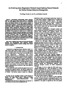
Game of dynamics Game of dynamics represents a discrete based version of the state space. It is defined from the generator. The equilibrium are determined from the game of dynamics. Conversion relation of the game of dynamics is {{x,y,z}} generated. Figure 1 describes I0 from a generator defined on {{x, y, z}}. (edges of the figure 1 a). According to the generator, x inhibits z and y activates z.

x

y

−

+

z

a) Regulatory network

∅

∅

x

y

z

x

y

z

x+y

x+z

y+z

x+y

x+z

y+z

x+y+z

x+y+z

b) Generator I0

c) Generation I0 {{x,y,z}}

Fig. 1. Example

We can notice that it exists a straightforward definition of the generator from the graphical representation used for gene regulatory networks. In usual + regulatory network, an activation is denoted by x → y whereas an inhibition − is denoted by x → y. These notations including levels are defined as follows (definition 9) with the conversion relations. According to the definition, the usual representation corresponds to the network described in figure 1.c . Definition 9 (Translation of classic regulatory arrows). k,+

∆

k,−

∆

x → y = kx I kx + y x → y = kx + y I kx n Preference. Conversions concern local interactions. Altogether they describe potential evolutions of the system according to local properties. In this framework, preference is used to select the effective trajectory induced by the regulation. Preference can be considered as a relation above conversion in order to disambiguate contradictory regulations. The generation process of conversion emphasizes contradictory regulation. Figure 1 shows an example. z is activated by x ( e.g. x I0 x + z) and z is inhibited by y (e.g. y + z I0 x). Respectively adding y to the first conversion and x to the second conversion gives rise to a contradictory regulation (e.g. x + y I x + y + z ∧ x + y + z I x + y). 7

A dilemma between two contradictory regulation (inhibition, activation) is typified by the following statement. Definition 10 (Dilemma). Let .· be a relation, a dilemma occurs iff: ∃X, ∃Y.X .· Y ∧ Y .· X

∅

∅

x

y

z

x

y

z

x+y

x+z

y+z

x+y

x+z

y+z

x+y+z

x+y+z

Fig. 2. Example of choices for dilemma in the preference relation

In figure 1, a bidirectionnal conversion is possible between synopsis x + y + z and y+z. The reciprocity comes from a contradictory control of the regulators on gene y. In one hand x inhibits z, on the other hand y activates z. The conversion cycle does not correspond to a realistic case because circuits in the graph of conversions is only due to an even number of elementary inhibitions. So the regulation of one gene should dominate the other. Hence, this case represents a case of dilemma that setting appropriate preference relation should and must disambiguate. In case depicted by figure 1, we must choose either the preference x + y B x + y + z (y dominates) or the preference x + y + z B x + y (x dominates). Both issues are described in figure 2. Direct edges correspond to the preference which are deduced from conversion whereas the curved edge corresponds to the preference which solves the dilemma. This has an impact on the equilibria because the set x + y + z is the equilibrium when the activation (y) dominates and the set y + z is selected when inhibition (x) dominates. A special attention should be paid to the dilemma, because they may reveal a specificity of the regulation according to environmental conditions. 3.1

Application to λ phage

The λ phage is a paradigmatic example of gene regulation. The reader can refer to [12] for details of the lambda phage and its modeling. Phage λ is a Temperate phage that infects Escherichia coli. One of two fates lysogeny and lysis awaits the λ-infected bacterium. In some cells the injected phage chromosome becomes 8

part of the host chromosome, this is called lysogeny stage. In other cells the phage chromosome enters the lytic cycle called lysis where the λ chromosome is extensively replicated and new phage particles are formed within the bacterium which leads to the death of the host cell [6]. The decision between lysis and lysogeny can be thought of as a switching mechanism. The stochastic switch is based upon a competition between the cro and cI genes. Cro prevents cI synthesis and it represses its own synthesis. As for cI, it represses the synthesis of cro and activates its own synthesis. Given the regulation between the cro and cI the tool generate the whole relations of conversions and preferences. This allows the computation of Equilibria. Figure 4 shows the graph representing the equilibria of the system. To model the interactions, we consider a single player. In the CP-game, variables x stands for the gene Cro and y for the gene CI. The generator is:  x + y I0 x inhibition      x + y I0 y inhibition x I0 2x self activation at level 1   2x I0 x self inhibition at level 2    ∅ I0 y By generating I from I0 , we find the following extended CP-Game (figure 3). The conversion relation contains extra dilemmas: – x + y I x and x I x + y (generated from ∅ I0 y) ; – 2x + y I 2x and 2x I 2x + y (generated from ∅ I0 y) – 2x + y I x + y and x + y I 2x + y (generated from x + y I0 y et I0 2x) Any conversion which does not correspond to a dilemma are also preferred. Moreover inhibitions which are sets of generators are preferred to activations. Two changes of mind equilibria exist which correspond to the steady states of the regulatory network found in literature: a loop and a steady state. ∅

∅

x

x

y

x+y

x+y

2x

y

2x

2x + y Conversions

2x + y Preferences

Fig. 3. λ phage regulatory CP Game

9

3.2

CP Game Notebooks

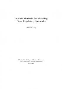
To validate the framework, we have developed a mathematica notebook [?] to test regulatory models 3 . Inhibitions and activations are translated to conversions. We briefly outline the main features of the environment. Mathematica code described in example 1 shows a typical use of functions contains in tne notebook. Figure 4 depicts a graphical representation of the change of mind relation and the equilibria are highlighted by different colors

Fig. 4. λ Phage - change of mind relation

Example 1 (Example of the use of the environment). First, the generator are described. conv0={0 -> ci, 0 -> cro, 2 cro -> cro, ci + cro -> ci, ci + cro -> cro}

Next the conversion are generated. conv = CPGenerate[conv0,{ci,2cro}] {0 -> ci, 0 -> cro, ci -> ci + cro, cro -> 2 cro, cro -> ci + cro, 2 cro -> cro, 2 cro -> ci + 2 cro, ci + cro -> ci, ci + cro -> cro, ci + cro -> ci + 2 cro, ci + 2 cro -> 2 cro, ci + 2 cro -> ci + cro}

Preferences are equivalent to conversions where dilemma which does not correspond to regulation are discarded, (e.g. the reverse of the conversions). p=CPStrict[ CPGenerate[CPReverse[{cro + ci -> cro, cro + ci -> ci}],{ci,2cro}]; pref=Complement[conv,p] {0 -> ci, 0 -> cro, cro -> 2 cro, 2 cro -> cro, ci + cro -> ci, ci + cro -> cro, ci + 2 cro -> 2 cro, ci + 2 cro -> ci + cro}

At least the CP equilibria are computed. From the change of mind relation a CP Equilibrium is : mind=Intersection[conv,pref]; eq = CPEq[mind] {{ci}, {cro, 2cro}} The description is relatively concise in comparison to the game of dynamics. In tested examples, the size is proportional to the number of involved genes. Indeed the description by games has the same complexity as the the description of gene regulatory network [10]. The result is depicted in figure 4 which show the graph of the change of mind relation and the equilibria. Equilibria are highlighted in different colors (red and blue). Synopsis belonging to the same equilibria have also the same color. The notebook offers us to test the framework for various examples. For instance, it has also been used to test the network of the PASsystem [4] [3]. 3

the notebook is freely available on request to the authors

10

4

Compositionality of the CP Game

** a ´ finir One of the main issue when a gene regulation system is analyzed through a model is to decompose the model into modules [9]. Predicting the action of a system relies on the ability to predict the different trajectories followed by the system. An important but challenging question is to determine the trajectory resulting from systems coupling. More specifically, we focus on the equilibria when systems are coupled. In CP Games, coupling two systems means composing games, and analyzing trajectories is based on equilibria analysis. Mastering the composition and decomposition of game is at the core a functional analysis of the dynamics. Indeed, each game can be viewed as the support of a specific function of the system under analysis. We are more specifically address the question of maintaining a synopsis as an equilibria. First, we formally define the composition of two CP games as an union of their components 11. Definition 11. let Γ = hA, S, (Ii ), (Bi )i and Γ 0 = hA0 , S 0 , (I0i ), (B0i )i be two CP games, we define: ∆

Γ ∪G Γ 0 = hA ∪ A0 , S ∪ S 0 , (Ii ∪ I0i )i∈A∪A0 , (Bi ∪ B0i )i∈A∪A0 i We denote ∪G by ∪ for simplicity. Determining whether a synopsis is an equilibrium (or being a member of a CP equilibrium) when games are composed is essential to predict the issue of a CP-Game. ** ´ a finir A first theorem concerns the abstract Nash equilibria. We prove that in this case equilibria are maintained by composition Proposition 2 (Abstract Nash Equilibria of CP Game Composition). aN aN EqaN Γ ∪Γ 0 (s) ⇒ EqΓ (s) ∨ EqΓ 0 (s) aN aN EqaN Γ ∪Γ 0 (s) ⇐ EqΓ (s) ∧ EqΓ 0 (s)

(1) (2)

Property 2 of proposition 2 proves the maintenance of a synopsis as an equilibrium when games are composed. An immediate consequence of theorem 2 concerns the cardinality of the abstract Nash equilibria(corollary 1). Corollary 1 (Cardinality of Composed Equilibria). Let Γ and Γ 0 be two games, the following inequality holds : |EaN (Γ ∪ Γ 0 )| ≤ |EaN (Γ )| + |EaN (Γ 0 )| However, proposition 2.2 cannot be generalized to CP equilibria. Theorem 1, proves that any synopsis belonging to a CP equilibrium, we can always find an other game where s also belongs to an equilibrium but not in their composition. Theorem 1 (Equilibria loss). CP CP 0 ∀Γ, ∀s ∈ S.EqCP Γ (bsc) ∧ bsc 6= {s} ⇒ ∃Γ .EqΓ 0 (bsc) ∧ ¬EqΓ ∪Γ 0 (bsc)

11

Proof. Given a game Γ = hA, S, (Ii ), (Bi )i, for any s such that EqCP Γ (bsc) holds and bsc 6= {s}, we define a game Γ 0 = hA0 , S 0 , (I0i ), (B0i )i as follows: – – – –

A = A0 ; S 0 = {s, s0 , z} with s0 ∈ bsc ∧ s0 6= s and z 6∈ S (Since bsc 6= {s}, s0 exists); ∀i ∈ A0 , s0 I0i z ∧ s0 I0i s; ∀i ∈ A0 , s0 B0i z ∧ s0 B0i s.

According to Γ 0 definition, the change of mind relation is s0 →0i z ∧ s0 →0i s for any player i. Hence we have EqCP Γ 0 (bsc). However by definition of composition of games we have ¬EqCP (bsc)  0 Γ ∪Γ

2x

2x x

2x + z

a) Γ.EqCP Γ (bxc) ∧ bxc 6= x

2x x

b) Γ 0 .EqCP Γ 0 (bxc)

2x + z

x

c) Γ ∪ Γ 0 .¬EqCP Γ ∪Γ 0 (bxc)

Fig. 5. Example of Equilibria loss

The lack of equilibria preservation is originally due to the lack of equivalence between the composition of reduced games and the reduced composed games (e.g. bΓ ∪ Γ 0 c 6= bΓ c ∪ bΓ 0 c in general). Hence theorems 1 and 2 cannot be extended to CP equilibria. However, some properties of CP Equilibria in the composed game can be deduced from games which compose it. Moreover, it is worth to point out that the computation of two strongly connected components from two different games may differ even they are identified by the same synopsis s (e.g. bscΓ 6= bscΓ 0 in general). Theorem 2 ( CP Equilibrium and Game Composition). CP CP EqCP Γ ∪Γ 0 (bsc) ⇒ ∃x ∈ bscΓ ∪Γ 0 .EqΓ (bxc) ∨ EqΓ 0 (bxc)

(3)

Theorem 2 is focused on the origin of equilibria in a composed game. The origin of an equilibria of the composed game comes at least from one equilibria or more issued from the initial games. Proposition 3 (CP-equilibria maintaining). CP CP EqCP Γ (bsc) ∧ EqΓ 0 (bsc) ∧ (bscΓ = bscΓ 0 ) ⇒ EqΓ ∪Γ 0 (bsc)

preuve

faire. 12

4.1

Composition and Generation

Proposition 4. Let G, G0 be two multisets, let Γ = hA, SM (G), (Ii ), (Bi )i and Γ 0 = hA0 , SM (G0 ), (I0i ), (B0i )i be two CP games, we have: Γ ∪ Γ0

G∪M G0

=Γ

G∪M G0

∪ Γ0

G∪M G0

From the proposition 4, we consider a set of generator to define a model. For instance different generators may correspond to pieces of the network and they are assembled together to form the CP Game corresponding to the network. Combining results concerning equilibria and those concerning generators. Hence, the combination of theorem 2 and proposition 4 leads to the following proposition. Proposition 5 (Equilibria and Generation). Let Γ and Γ 0 be two game with the same synopsis, SM (G) CP CP G .Eq EqΓCP G (bsc) ⇒ ∃x ∈ bsc G (bxc) ∨ Eq 0 G (bxc). Γ ∪Γ 0 ∪Γ 0 Γ Γ

EqaN Γ ∪Γ 0 EqaN Γ ∪Γ 0

G

(s) ⇒

G

(s) ⇐

EqaN G (s) Γ aN EqΓ G (s)

∨ ∧

EqaN G (s) Γ0 aN EqΓ 0 G (s)

(4) (5) (6)

To complete the analysis with the generation, we need to establish a connection between the generator and the generated game. The following theorem gives the necessary connexion

5

Conclusion

In this section, we introduce a new framework based on CP-Game to analyse the dynamics of gene regulatory network. The model is based on the notion of generators which provides an unified formalism to express two fundamental representation underpinning the dynamics studies : the description of the interactions, and the discrete based representation of the dynamics. To summarize the analysis, The description of the representation is relatively concise ** ´ a finir

References 1. Claudine Chaouiya, Elizabeth Remy, and Denis Thieffry. Petri net modelling of biological regulatory networks. Proceedings of CMSB-3, 2005. 2. C. Chettaoui, F. Delaplace, P. Lescanne, M. Vestergaard, and R. Vestergaard. Rewriting game theory as a foundation for state-based models of gene regulation. In Computational Methods in Systems Biology, volume 4210 of Lecture Notes in Computer Science, pages 257–270. Springer Verlag, 2006. 3. C. Chettaoui, M. Delaplace, F.and Manceny, and M. Malo. Games network and application to pas system. Biosystems, In Press, 2006.

13

4. M. Malo, C. Charrire-Bertrand, C. Chettaoui, E. Fabre-Guillevin, F. Maquerlot, A. Lackmy, B. Valle, D. Delaplace, and G. Barlovatz-Meimon. Microenvironnement cellulaire, pai-1 et migration cancreuse. Comptes Rendus Biologies, 329:919–927, December 2006. 5. M. J. Osborne and A. Rubinstein. A Course in Game Theory, volume 380. MIT Press, 1994. 6. M. Ptashne. A Genetic Switch, Phage lambda and Higher Organisms. Cell Press and Blackwell Publishing, 1992. 7. St´ephane Le Roux, Pierre Lescanne, and Ren´e Vestergaard. A discrete Nash theorem with quadratic complexity and dynamic equilibria. Research Report IS-RR2006-006, JAIST, May 2006. 8. MA. Savageau and F.C. Neidhart. Regulation beyond the operon. in escherichia coli and salmonella typhimurium: Cellular and molecular biology (ed. neidhart, f.c.). American Society for Microbiology, Washington D.C., 1:1310–1324, 1996. 9. E. Segal, M. Shapira, A. Regev, D. Pe’er, Botstein D., and Koller D. Module networks: indentiflying regulatory modules and their condition-specific regulators from gene expression data. Nature Genetics, 34(2):166–176, 2003. 10. D. Thieffry and R. Thomas. Dynamical behaviour of biological regulatory networks-II. Immunity control in bacteriophage lambda. Bulletin of Mathematical Biology, 57(2):277–297, 1995. 11. R. Thomas. Boolean formalization of genetic control circuits. Journal of Theoretical Biology, 42(3):563–585, 1973. 12. R. Thomas. Regulatory networks seen as asynchronous automata: A logical description. Journal of Theoretical Biology, 153, 1991.

14

Annex : Prove of Theorems and propositions Proof. of theorem 2, equation 1: 0 0 0 0 0 EqaN Γ ∪Γ 0 (s) ⇒ ∀i ∈ A ∪ A , ∀s ∈ S ∪ S .s Ii s ⇒ ¬s Bi s

s ∈ S ∪ S 0 so s ∈ S or s ∈ S 0 . Two cases must be considered: 0 0 0 0 0 EqaN Γ ∪Γ 0 (s), s ∈ S ⇒ s ∈ S, ∀i ∈ A ∪ A , ∀s ∈ S ∪ S .s Ii s ⇒ ¬s Bi s ⇒ s ∈ S, ∀i ∈ A ∪ A0 , ∀s0 ∈ S(⊂ S ∪ S 0 ).s Ii s0 ⇒ ¬s Bi s0 ⇒ EqaN Γ (s)

or 0 0 0 0 0 0 0 EqaN Γ ∪Γ 0 (s), s ∈ S ⇒ s ∈ S , ∀i ∈ A ∪ A , ∀s ∈ S ∪ S .s Ii s ⇒ ¬s Bi s ⇒ s ∈ S 0 , ∀i ∈ A ∪ A0 , ∀s0 ∈ S(⊂ S ∪ S 0 ).s Ii s0 ⇒ ¬s Bi s0 ⇒ EqaN Γ 0 (s)

the theorem is immediately deduced from the both cases: aN aN EqaN Γ ∪Γ 0 (s) ⇒ EqΓ (s) ∨ EqΓ 0 (s)

 Proof. of theorem 2, equation 2: By definition we have : 0

0

0

0

IΓi ∪Γ =IΓi ∪ IΓi BΓi ∪Γ =BΓi ∪ BΓi So we can deduce that:

aN 0 0 0 EqaN Γ (s) ∧ EqΓ 0 (s) ⇒ (∀i ∈ A, ∀s ∈ S.s Ii s ⇒ ¬s Bi s ) ∧ (∀i ∈ A0 , ∀s0 ∈ S 0 .s Ii s0 ⇒ ¬s Bi s0 ) ⇒ ∀i ∈ A, ∀j ∈ A0 , ∀s0 ∈ S, ∀s00 ∈ S 0 .(s Ii s0 ⇒ ¬s Bi s0 ) ∧ (s Ij s00 ⇒ ¬s Bj s00 ) ⇒ ∀i ∈ A, ∀j ∈ A0 , ∀s0 ∈ S, ∀s00 ∈ S 0 .(s Ii s0 ) ∨ (s Ij s00 ) ⇒ (¬s Bi s0 ) ∨ (¬s Bj s00 ) ⇒ ∀i ∈ A, ∀j ∈ A0 , ∀s0 ∈ S ∪ S 0 .(s(Ii ∪ Ij )s0 ) ⇒ (¬s (Bi ∪ Bj )s0 ) 0

0

⇒ ∀i ∈ A ∪ A0 , ∀s0 ∈ S ∪ S 0 .s IΓi ∪Γ s0 ⇒ ¬s BΓi ∪Γ s0 ⇒ ∀i ∈ A ∪ A0 , ∀s0 ∈ S ∪ S 0 .s Ii s0 ⇒ ¬s Bi s0 ⇒ EqaN Γ ∪Γ 0 (s)  15

Proof. of proposition 3: CP EqCP Γ (bsc) ∧ EqΓ 0 (bsc) ∧ (bscΓ = bscΓ 0 ) aN ⇒ EqaN bΓ c (bsc) ∧ EqbΓ 0 c (bsc) ∧ (bscΓ = bscΓ 0 )

⇒ (∀i ∈ A, ∀bs0 c ∈ bΓ c.bsc Ii bs0 c ⇒ ¬bsc Bi bs0 c) ∧ (∀i ∈ A0 , ∀bs0 c ∈ bΓ 0 c.bsc Ii bs0 c ⇒ ¬bsc Bi bs0 c ∧ (bscΓ = bscΓ 0 ) ⇒ (∀i ∈ A, ∀bs0 c ∈ bΓ c.bsc Ii bs0 c ⇒ ¬bsc Bi bs0 c) ∧ (∀i ∈ A0 , ∀bs0 c ∈ bΓ 0 c.bsc Ii bs0 c ⇒ ¬bsc Bi bs0 c) ∧ (bscΓ = bscΓ 0 ) Proof. of theorem 2, equation 3: aN EqCP Γ ∪Γ 0 (bsc) ⇒ EqbΓ ∪Γ 0 c (bsc)

⇒ ∀i ∈ A, ∀bs0 cbΓ ∪Γ 0 c .bscbΓ ∪Γ 0 c Ii bs0 cbΓ ∪Γ 0 c ⇒ ¬bscbΓ ∪Γ 0 c Bi bs0 cbΓ ∪Γ 0 c We generate 4 cases where two are always satisfied. (we don’t consider these two cases). aN EqCP Γ ∪Γ 0 (bsc) ⇒ EqbΓ ∪Γ 0 c (bsc)

⇒ ∃x ∈ bscΓ ∪Γ 0 .bxc ∈ bΓ c, ∀i ∈ A, ∀bs0 cΓ ∪Γ 0 , ∃y ∈ bs0 cΓ ∪Γ 0 .byc ∈ bΓ c. bxcbΓ ∪Γ 0 c Ii bycbΓ ∪Γ 0 c ⇒ ¬bxcbΓ ∪Γ 0 c Bi bycbΓ ∪Γ 0 c ⇒ ∃x ∈ bscΓ ∪Γ 0 , ∀i ∈ A, ∀bycΓ . bxcbΓ c Ii bycbΓ c ⇒ ¬bxcbΓ c Bi bycbΓ c ⇒ ∃x ∈ bscΓ ∪Γ 0 , ∀i ∈ A, ∀bycΓ . bxcbΓ c Ii bycbΓ c ⇒ ¬bxcbΓ c Bi bycbΓ c ⇒ ∃x ∈ bscΓ ∪Γ 0 , EqaN bΓ c (bxc) Or aN EqCP Γ ∪Γ 0 (bsc) ⇒ EqbΓ ∪Γ 0 c (bsc)

⇒ ∃x ∈ bscΓ ∪Γ 0 .bxc ∈ bΓ 0 c, ∀i ∈ A, ∀bs0 cΓ ∪Γ 0 , (∃y ∈ bs0 cΓ ∪Γ 0 . byc ∈ bΓ 0 c).(bxcbΓ ∪Γ 0 c Ii bycbΓ ∪Γ 0 c ⇒ ¬bxcbΓ ∪Γ 0 c Bi bycbΓ ∪Γ 0 c ⇒ ∃x ∈ bscΓ ∪Γ 0 , ∀i ∈ A, ∀bycΓ 0 . bxcbΓ 0 c Ii bycbΓ 0 c ⇒ ¬bxcbΓ 0 c Bi bycbΓ 0 c ⇒ ∃x ∈ bscΓ ∪Γ 0 , ∀i ∈ A, ∀bycΓ 0 . bxcbΓ 0 c Ii bycbΓ 0 c ⇒ ¬bxcbΓ 0 c Bi bycbΓ 0 c ⇒ ∃x ∈ bscΓ ∪Γ 0 , EqaN bΓ 0 c (bxc) 16

It follows that: CP CP EqCP Γ ∪Γ 0 (bsc) ⇒ ∃x ∈ bscΓ ∪Γ 0 .EqΓ (bxc) ∨ EqΓ 0 (bxc)



17