Deformable 3âD models can be represented either as explicit or implicit ... We demonstrate the ap- plicability of our technique for upper bodyâhead, neck and .... mechanism that looses the algebraic nature of the distance function and makes ...
Generic Deformable Implicit Mesh Models for Automated Reconstruction Slobodan Ilic, Pascal Fua Swiss Federal Institute of Technology Computer Vision Laboratory IN-J Ecublens, 1015 Lausanne, Switzerland {Slobodan.Ilic, Pascal.Fua}@epfl.ch Abstract Deformable 3–D models can be represented either as explicit or implicit surfaces. Explicit surfaces, such as triangulations or wire-frame models, are widely accepted in the Computer Vision and Computer Graphics communities. However, for automated modeling purposes, they suffer from the fact that fitting to 2–D and 3–D image-data typically involves minimization of the Euclidean distance between observations and their closest facets, which is a nondifferentiable distance function. By contrast, implicit surface representations allow fitting by minimizing an algebraic distance where one only needs to evaluate a differentiable field potential function at every data point. However, they have not gained wide acceptance because they are harder to meaningfully deform and render. To combine the strength of both approaches, we propose a method that can turn a completely arbitrary triangulated mesh, such as one taken from the web, into an implicit surface that closely approximates its shape and can deform in tandem with it. This allows both graphics designers to deform and reshape the implicit surface by manipulating explicit surfaces using standard deformation techniques and automated fitting algorithms to take advantage of the attractive properties of implicit surfaces. We demonstrate the applicability of our technique for upper body—head, neck and shoulders— automated reconstruction.
1. Introduction In the world of Computer Graphics, 3–D objects tend to be modeled as explicit surfaces such as triangulated meshes or parametric surfaces like spline patches. Because such representations are intuitive and easy to manipulate, they This work was supported in part by the Swiss National Science Foundation.
are widely accepted among graphics designers. These representations, however, are not necessarily ideal for fitting surfaces to data such as 3–D points produced by laserscanners and stereo systems or 2–D points from image contours where the data are noisy and incomplete. This stems from the fact that fitting typically involves finding the facets that are closest to the 3–D data points or most likely being silhouette facets. This involves non-differentiable distance function, which degrades the convergence properties of most optimizers. Implicit surfaces, known in the literature as Blobby Molecules[4], Soft Objects[34] and Metaballs[19], have received substantial attention in both the Computer Graphics and Computer Vision communities. They are well-suited for simulating physically based processes and for modeling smooth objects. Because the algebraic distance to an implicit surface is computed by evaluating a differentiable function, they do not suffer from the drawbacks discussed above when it comes to fitting them to 2 and 3–D data [29, 22, 8]. However, they have not gained wide acceptance, in part because they are more difficult to deform and to render than explicit surfaces. In short, explicit surface representations are well suited for graphics purposes, but less so for fitting and automated modeling. The reverse can be said of implicit surface representations. In earlier work [?], we proposed method for combining the strengths of both approaches while avoiding their drawbacks by converting explicit surfaces into implicit meshes whose shape closely approximates that of the original triangulations and deforming the implicit and the explicit surfaces in tandem for fitting purposes. To create the implicit mesh, we circumscribed each facet with a spherical volumetric primitive with its center being on the facet, as depicted by the middle row of Fig. 1. This approach is effective but has some limitations: It works best for fairly regular meshes like one shown in the middle row of Fig. 1, or high-resolution meshes such as one shown in Fig. 2(e, f), while it can produce lumpy implicit surfaces for irregular coarse ones, as depicted in Fig. 2(a, b).
Figure 1. Converting an explicit surface into an implicit surface. Top row: Initial explicit meshes (facet, triangulated mesh patch and deformed mesh patch, from left to right respectively) . Middle row: Initial explicit surfaces from the top row converted to the spherical implicit meshes shown as transparent around explicit once. Bottom row: Initial explicit surfaces from the top row converted to the triangular implicit meshes shown again as transparent.
Here, we overcome these limitations by replacing spherical metaballs by triangular metaballs shown in the left hand side image of the bottom row in Fig. 1. Instead of computing the potential field as a function of the distance from the center of a facet, we take it to be the Euclidean distance from the whole triangle. As shown in the bottom row of Fig. 1 and in third and forth column of Fig. 2, the thickness of the implicit surface approximating the explicit surface can be arbitrarily small, whatever the mesh topology. The parameters of those metaballs are a function of the facet geometry. As a result, when a facet deforms, so does the corresponding metaball and the implicit and the explicit surfaces move in tandem. In this work, we use Dirichlet Free Form Deformation(DFFD) [18, 13] to control the shape, but in general, since we can turn any mesh into its implicit representation one could have chosen other methods, such as Free Form Deformations(FFDs) [26, 7], B-splines or PCA parameterization [3] to deform the explicit mesh and consequently the implicit one. DFFD had been chosen because it allows us to control any complex shapes with a relatively small number of parameters, then allows arbitrary control points deploy-
ment, produces local deformation and provides very natural way of deforming the objects for the graphics designers. Our contribution is therefore an approach to surface fitting that allows to take an arbitrary explicit surface model of any complexity, for example one that has been obtained from the web and was not designed with fitting in mind, turn it into an implicit mesh, and deform it to obtain an optimal fit to image-data. In the automatic reconstruction implicit surface is just virtually present and it was fitted to the data, while actual explicit mesh was deformed along with it. Because of very close approximation of the mesh with its virtual implicit surface we can keep the deformed explicit mesh and use it instantly for rendering, furthermore provide it to the graphic designer with a optimal position of the control points for further modification and animation. In the remainder of the paper, we first briefly review earlier approaches. We then introduce our approach to creating implicit meshes and deforming them, where we compare spherical and new triangular metaballs approach. Then, we describe our optimization framework, and finally demonstrate the applicability of our framework to the complex
case of fitting the upper-body including – head, neck and shoulders – to image-data, where we compare results obtained by fitting explicit mesh, spherical implicit mesh and triangular implicit mesh to stereo and silhouette data.
2. Previous Work Three-dimensional surface reconstruction continues to be an important goal and many approaches relying on explicit surface representations, such as 3–D surface meshes [6, 31], parameterized surfaces [28, 17], local surfaces [10], and particle systems [30], have been proposed. There has also been sustained interest in the use of volumetric primitives [16, 31, 20] and implicit surface representations [8, 29, 23] for fitting purposes. These methods, however, are tailored for specific shapes such as the human body and its skeleton and there is no generally accepted way to deform generic implicit surfaces. A popular way to deform implicit surfaces is to twist, bend, and taper the space in which the model lives by choosing a suitable warping function [4, 2, 33]. However, these deformations are limited to parametric surfaces, such as spheres or cylinders, and there is no way to warp the space in a free form manner. In [1], simple superquadrics are parametrized using conventional FFDs for automatic heart reconstruction and deformation from medical images. Here the FFDs ability to deform parametric surfaces has been exploited, but only to reshape a single primitive. Our proposed implicit shells coupled with DFFDs [18, 13] go much further by allowing us to deform completely generic implicit surfaces. In spirit, the our implicit meshes are related to the earlier distance surfaces [5]. However, in this earlier work, the problems associated to bulges created by metaballs blending into each other are handled by a convolution mechanism that looses the algebraic nature of the distance function and makes the distance surfaces impractical for the kind of fitting we perform. Radial basis functions (RBF) [14, 15, 32] are an interesting alternative to soft objects or metaballs [34, 19]. The shape of the resulting surface, however, is controlled not only by the position of the RBF centers but also by the RBF weights that have no geometric interpretation, which makes this approach also unsuitable for in-tandem deformation of explicit and implicit surface. In short, both approaches to 3–D modeling have their strengths and weaknesses for the purpose of fitting noisy image-data. It is therefore important to be able to combine two kinds or representations and deform them in tandem.
3. Implicit Mesh Models To create an implicit mesh model that can deform in tandem with the explicit surface, we must address two prob-
lems: 1. Creating an implicit surface that closely approximates the shape of the initial explicit mesh, 2. Controlling the object shape, in both its explicit and implicit forms, using the same set of parameters. To convert an arbitrary triangulated surface into an implicit mesh, we create an implicit surface primitive or metaball for each facet. In earlier work [?] we used spherical metaballs, which are very simple but only suitable for fairly regular meshes or high resolution meshes as it is shown in the middle row of Fig. 1, where first one triangle, then ordinary regular and the deformed mesh patch are converted into spherical implicit mesh shown as transparent. Here, we replace them by the triangular metaballs, which are more complex but can handle arbitrarily irregular meshes and low resolution meshes and perform much closer approximation of the explicit surface, as depicted by the third row of Fig. 1. In this section, we first compare the two kinds of metaballs and then discuss our approach to shape deformation.
3.1. Spherical Metaballs The spherical metaball [?] is created by circumscribing a spherical primitive around a facet in such a way that the sphere center lies on the facet and corresponds to the center of the circumscribed circle around the facet. It defines a potential field that can be expressed as:
������� ��
������������������������ ��� (1) � � where is a 3–D � � point, is the Euclidean distance to the sphere’s center, is the radius of the spherical metaball and � is free coefficient defining slope of the potential field function. The implicit mesh, shown in gray in the middle row of Fig. 1, is then taken to be an isosurface of the sum of all these potential � fields. Formally, it is defined as the set of 3–D points that satisfy
�
% $ % � ����� � �!�#" '�(�����)��� �� �����*�+�,� & �
,
(2)
where is an arbitrarily chosen isovalue. Usually we take � to be one, so that all points on the surface have a potential field value equal to zero and the values smaller then zero inside and greater then zero outside. Because the spherical metaballs are circumscribed around the facets their ra�+� dius depends on the size of the triangle. As shown in the second row of Fig. 1, as long as the explicit mesh is relatively regular or high resolution, this yields a valid approximation. However, because large facets produce large primitives, the approximation becomes much less accurate when the explicit mesh has large facets. If we deal with low resolution irregular mesh as the one depicted in Fig. 2(a),
(a)
(b)
(c)
(d)
(e)
(f)
(g)
(h)
Figure 2. Conversion of low and high resolution explicit meshes to implicit ones, using either spherical or triangular metaballs . Left column(a, e): Low and high resolution mesh. Second column(b, f): Corresponding implicit surfaces created with spherical metaballs, shown as transparent. Third column(c, g): Corresponding implicit surfaces created with triangular metaballs. Last column(d, h): Magnified implicit triangular metaballs surface in the neck and shoulders area, highlighting the approximation’s quality.
elongated facets produce an implicit surface whose thickness can change dramatically, as shown in Fig. 2(b). Up to a point, that can be remedied by retriangulating the mesh obtaining one depicted in Fig. 2(e), so that it consists of many smaller size facets and produce better approximation as shown in Fig. 2(f). This has been done in our previous work [?], but of course, that results in a substantial increase in computational cost. Lack of close approximation of the explicit mesh with the implicit one may produce problems during the fitting. That is caused by the notion of two sides of the implicit surface which become important when implicit surface is thick like in a case of spherical implicit surface depicted in Fig. 3(a). If the model is not encapsulated inside the observation data and it intersects with the observations, that can cause fitting of the wrong side of the implicit surface to the data as it is shown in Fig. 3(b) in the neck area.
3.2. Triangular Metaballs To solve these problems, and create implicit surfaces that more closely approximate arbitrary meshes, we propose to replace the spherical metaballs by triangular ones. This is � done by replacing the Euclidean distance to the facet’ center in Eq. 1 by the actual distance - to the whole facet. In the bottom row of Fig. 1 you can see metaball created around the triangle which we call triangular metaball. The distance function is the Euclidean distance from the triangle expressed as function which defines distance either from the plane if the point projects on the triangle or the distance from the line or point if the point project outside the triangle. Finally, distance function can be incorporated in the same potential field function as used for spherical metaballs:
(a)
(b)
(c)
(d)
Figure 3. Influence of the explicit mesh approximation by the spherical or triangular implicit surface to fitting results. (a) Spherical implicit mesh. (b) Inner side of the spherical implicit mesh fitted to the data, depicted as small circles, in the neck area. (c) Triangular implicit mesh. (d) Correct fitting of triangular implicit mesh to the data because of the small thickness of the implicit surface.
������� �
�������������������� -
3.3. Deforming Implicit and Explicit Meshes
� �.�
(3)
�/�� 0�
that has almost the same form as before, but where is � distance of the point in space to the triangle and - is a distance that represents the thickness of the implicit � surface. Actually, all the points in space at the distance - from the triangle have potential field value equal to zero. Again, complete implicit surface is obtained by summing all the field potentials that produces overall implicit surface expressed as:
% $ % � �����1�!�!� " '�(�����)��� �� ���2� � � & �
,
(4)
It is easy to spot that the potential field is now independent of the facet sizes and mesh resolution as depicted in Fig. 2(c, g, d, h) what is not the case for the spherical metaballs as shown in Fig. 2(b, f). Having control over the pa� rameter - allows us to approximate the explicit mesh with an arbitrarily thin implicit surface and in that way to relax the constraint of using fairly regular or high resolution mesh. However, triangular implicit mesh might produces small bulges near vertices and along the edges, but since we have � control over the slope of the exponential� field function it is easy to remove the bulges by tuning to smaller value. Also, the problem of fitting to the wrong side of the implicit surface is now overcome by the � very close approximation of explicit surface. Choosing - to be arbitrary small thickness of the implicit surface, even if fitting is done to the inner side of it, fitting error is negligible as shown in Fig. 3(c, d).
We have shown that introducing DFFD control points is an effective way to deform explicit meshes [13]. Our idea of converting explicit mesh to implicit surface by close approximation allows to apply the same deformation mechanism based on DFFD control points to control the shape of both explicit and implicit surface. 3.3.1. Deforming Explicit Meshes Mayor advantage of DFFD over other FFDs [26, 7, 12], is obtained by releasing the constraint on the shape of the control mesh, which is the main conceptual geometric limitation of FFDs. Here rectangular local coordinates of FFDs are replaced by generalized natural neighbor coordinates of DFFD, also known as Sibson coordinates, and a generalized interpolant [9] is applied. The idea comes from the data visualization community that relies on data interpolation and, thus, heavily depends on local coordinates. This property of locality allows using sparse matrix computation in our optimization framework, what is not the case for other FFDs which are global deformation. 3.3.2. Computing Sibson Coordinates Every surface triangulation point is influenced by certain subset of control points. The magnitudes of these influences, known as Sibson coordinates [27], are computed only once before the optimization starts [18]. The displacement of each surface triangulation point is the linear combination of the displacements of the control points that influence it. �54 3268793��F :�7+;