2. deforming the implicit and the explicit surfaces in tan- dem for fitting purposes as ..... Let pЩiyСt be the point on the line of sight where it is tan- gential to niyСt .
Implicit Meshes for Modeling and Reconstruction Slobodan Ilic and Pascal Fua Computer Vision Laboratory, EPFL, Switzerland {Slobodan.Ilic, Pascal.Fua}@epfl.ch
Abstract Explicit surfaces, such as triangulations or wireframe models, have been extensively used to represent the deformable 3–D models that are used to fit 3–D point and 2–D silhouette data. The resulting approaches, however, suffer from the fact that fitting typically involves finding the facets that are closest to the 3–D data points or most likely to be silhouette facets. This requires searching, which is slow, and dealing with the non-differentiability of the distance function. By contrast, implicit surface representations allow fitting without search, since one can simply evaluate a differentiable field function at every data point. However, implicit representations are not necessarily the most intuitive ones and users, such as graphics designers, tend to prefer explicit models.
1. Introduction Explicit surfaces, such as triangulations or wireframe models, have been extensively used to represent the deformable 3–D models that are used to fit 3–D point and 2–D silhouette data. The resulting approaches, however, suffer from the fact that fitting typically involves finding the facets that are closest to the 3–D data points or most likely to be silhouette facets. This requires searching, which is slow, and dealing with the non-differentiability of the distance function—for example, when a point that was associated to one facet becomes attached to a different one—that may hinder the minimization of the criterion being used. By contrast, implicit surface representations allow fitting without search, since one only needs to evaluate a differentiable field function at every data point [20, 14]. However, implicit representations are not necessarily the most intuitive ones, and graphics designers, tend to prefer explicit models. Furthermore, for some classes of algorithms such as shape-from-shading methods, explicit representations seem better suited to the problem.
(a)
(b)
(c)
(d)
Figure 1. Turning the explicit surface into an implicit shell. (a) Initial explicit mesh with control points shown as squares. (b) Mesh converted into implicit shell. (c) Deformed mesh after displacement of the control points. (d) The implicit shell follows the explicit surface.
In this paper, we propose to combine the strengths of both approaches by: 1. transforming explicit surfaces into implicit shells, which we call implicit mesh models, whose shape closely approximates that of the original triangulations as depicted by Figure 1(a,b).
�
2. deforming the implicit and the explicit surfaces in tandem for fitting purposes as shown in Figure 1(c,d).
This work was supported in part by the Swiss Federal Office for Education and Science
1
Figure 2. Reconstruction from an uncalibrated video sequence. Top row: 3 of 6 images from a short video sequence with overlaid silhouettes. Middle row: Disparity maps extracted from rectified consecutive image pairs using max flow-based stereo, after automated registration. Bottom row: Reconstructed and textured models obtained by using an explicit model for the head and an implicit mesh model for the neck and shoulders.
To create the implicit shell, we circumscribe each facet with a spherical volumetric primitive. We will show that, if the triangulation is sufficiently well-behaved, the resulting shell closely approximates the mesh. To deform both representations simultaneously, we follow the Free Form Deformation (FFD) paradigm that lets us embed both kinds of models in a volume whose shape can be changed by moving control points. In particular, we advocate the use of Dirichlet Free Form Deformations (DFFDs) [12] because, unlike conventional FFDs, they do not require the control points to lie on a regular rectangular grid. This is achieved by replacing the standard rectangular local coordinates by generalized natural neighbor coordinates, also known as Sibson coordinates [18]. It gives us the ability to place control points at arbitrary locations rather than on a regular lattice, and thus, much greater flexibility. In practice, control points are taken to be on the surface triangulation, with a denser distribution where the surface curvature is high. Our contribution is therefore an approach to surface fit-
ting that allows us to take an arbitrary explicit surface model, for example one that has been obtained from the web and was not designed with fitting in mind, turn it into an implicit shell, and deform it to obtain an optimal least-square fit to new experimental data using a few well-chosen control points. In Figure 2, we demonstrate the power of this approach for upper-body modeling using stereo and silhouette data. The model we use has a complex topology, but that complexity has no impact on the quality of the fitting. We first relate our techniques to existing ones. We then introduce our approach to creating implicit shells and to deforming them using DFFDs. Finally, we demonstrate the applicability of our framework.
2. Related Work 2.1. Explicit versus Implicit Three-dimensional reconstruction of visible surfaces continues to be an important goal of the computer vision
research community and many approaches relying on full 3–D explicit representations have been proposed, such as 3– D surface meshes [4, 23], parameterized surfaces [19, 11], local surfaces [6], and particle systems [21]. In parallel, there has also been sustained interest in the vision community in the use of volumetric primitives [13, 10, 22] and implicit surface representations [5, 20, 15]. In the computer graphics community, approaches to interpolating explicit surfaces with implicit ones using radial basis functions (RBF) have been proposed [3, 24]. However, the shape is controlled not only by the position of the RBF centers but also by the RBF weights that have no geometric interpretation, which makes this approach unsuitable for the kind of optimization we contemplate here. This is why we have developed a different approach to converting explicit surfaces into implicit shells that guarantees that the implicit shell’s shape deforms exactly in the same way as the explicit surface. Both approaches to 3–D modeling have their strengths and weaknesses for the purpose of fitting noisy image-data. Explicit surfaces are easy to deform and to render using well known computer graphics techniques, but as discussed earlier, are not ideal for fitting purposes. Implicit surfaces are better suited for least-squares style fitting purposes because they can be used to define differentiable objective functions [20, 14]. However, unless one uses either a single geometric primitive or a set of such primitives attached to some kind of skeleton, it is relatively difficult to control their shape in an intuitively pleasing way. As a result users such as graphics designers tend to prefer explicit models. It is therefore important to be able to go back and forth between the two kinds or representations.
2.2. Deforming the Surfaces Free Form Deformations (FFDs) are a well-known approach to deforming 3–D models, explicit or implicit, by warping the space in which they exist [17]. However, a serious restriction is that FFDs can be naturally applied only to explicit surfaces and to parametric implicit surfaces such as quadrics or superquadrics. There is no generally accepted way to handle more complex implicit surfaces such as the implicit shells we are dealing with in this paper. Another popular and closely related way to deform implicit surfaces is to twist, bend, and taper the space in which the model lives by choosing a suitable warping function [1, 25, 2]. But, again, this only works for implicit surfaces with parametric descriptions. Because the shape of the implicit shell depends only on the shape of the explicit surface it is derived from, we can use any Free Form Deformation technique. Here we advocate the use of Dirichlet Free Form Deformations[12]. In previous work [8], we showed that it is effective to fit ex-
plicit surfaces to noisy data. In this paper, we extend our earlier approach so that it can handle both explicit and implicit surfaces.
3. Implicit Mesh Models To create an implicit surface model that can deform in tandem with the explicit surface, we must address two problems: 1. Creating an implicit shell that closely approximates the shape of the initial explicit mesh, 2. Controlling the object shape, in both its explicit and implicit forms, using the same set of parameters. Our approach is depicted by Figs. 1 and 3. We now discuss its components.
3.1. From Explicit Surface to Implicit Shell We first build an implicit shell whose shape approximates the initial explicit mesh as follows. We circumscribe a spherical metaball primitive around each facet of the surface triangulation in such a way that the sphere center lies on the facet as shown in the upper row of Fig. 3. Ideally, to get a smooth implicit surface, the explicit mesh should have equally sized facets. In practice, the smaller the facets, the smaller the spheres circumscribed around them, and the closer the resulting implicit mesh approximates the initial explicit mesh. We have therefore found experimentally that subdividing the explicit mesh until all the facets are small enough is sufficient to produce visually pleasing results. The bottom row of Fig. 3 depicts the conversion of a simple regular triangulation patch into an implicit mesh. Furthermore, as will be discussed below, the number of control parameters does not depend on the number of primitives and there is no significant computational penalty in so doing.
3.2. Deforming Explicit Meshes We have shown in earlier work that introducing DFFD control points is an effective way to deform explicit meshes [8]. These points can be distributed freely in space and every surface triangulation point is influenced by certain subset of control points. The magnitudes of these influences, known as Sibson coordinates [18], are computed before the optimization starts [12]. The displacement of each surface triangulation point is the linear combination of the displacements of the control points that influence ������� � � � � �� ���� it. Let be the set of control points and � be a subset influencing surface triangulation point � , ��� ��� ����� ����� , where !�#" � ��� �$�&%(' . The elements
P
L
of primitive R , and is the radius of primitive and S is the number of spherical metaballs. Note that, number of parameters is the number of control points and does not depend on number of facets. We experimented with two different potential field functions. The first one is piecewise polynomial:
L L Lcb L PX`aP J 3L � P P � YE K < J2_ � P P(`aP L 3 P��QP J U V XW Z � E[\W0E P K P J ^ EM � K ] P(eaP 3 ]�d0 " ]�d0 (3) P where is the distance of point f to the center of the primiT
L
tive. The plot of this function in Fig 4 (a) shows that on the sphere’s surface, the primitive potential field is 1, it grows when approaching the center, and monotonically decreases until it reaches " .
Figure 3. Converting an explicit surface into an implicit mesh. Upper row: Single triangular primitive on the left, converted to the transparent spherical metaball primitive on the right. Bottom row: Regular explicit surface patch on the left, converted to the transparent implicit mesh on the right
Parabolic potential field function 7
6
5
4 f(r)
k=3.0
3
of � are the natural neighbors of �
k=1.0
and� their influence is expressed by the Sibson coordinates ) . Let the control points from their initial positions by * ���+� from ��� � � be � � %(displaced ' ,�#" . The new position of the surface triangulation point becomes:
� 4 5 � * � �+�&� �( �.-0/21 � �(3 � 7� 698 )
� 4 � �76;8 ) = with : �
"
2
1 k=0.6
0
0
1
2
3 R0
4
5
R1
R2
6
7
8 r
Exponential potential field function 4.5
(1)
4
3.5
.
3
2.5
2
Our goal is to deform the implicit mesh in tandem with the explicit meshes. Each spherical primitive being circumscribed around a facet so that its center lies on the facet, both its center and its radius depend only on the facet vertices. These locations, in turn, can as a funcA ? expressed AC� �9?&@ �Bbe tion of the DFFD control points of Eq. 1. We can therefore write the field function D that defines the implicit shell as
D!EGF
� � � � �H�I�&� ��J L
���
k=3.0
f(r)
3.3. Deforming Implicit Meshes
L
L
J �QP J � 5L �=< � " K 6 � M EON EOF
(2)
where F is a point in , M is one of the field functions discussed below, N is the Euclidean distance to the center
k=1.0
1.5
k=0.6
1
0.5 T 0 1.5
2
2.5
3
3.5
4
4.5
5
r
Figure 4. Potential field functions. Top: Piecewise potential field function. Bottom: Exponential potential field function. In both cases, the parameter controls the size of the zone of influence of the primitives and, thus, the amount of smoothing.
L The parameter of Eq. 3 controls the zone of influence of the primitives. As decreases, the zone’s size becomes larger and the resulting implicit surface grows both smoother and larger, as shown on the top graph of Fig. 4. On the contrary when increases, the zone of influence becomes smaller and the implicit surface approximates more closely the explicit mesh. This function is good from a computational point of view, because the potential for a particular 3–D point can be calculated only from the subset of primitives spheres in whose zone of influence it belongs. However, for fitting purposes, this can cause problems when the initial model is not close enough from the data that can then end up being completely ignored. Therefore, we use instead an exponential potential field function: L L
M E
P�� P J
P P JQJ �hg ikj9E2Kl\W0E K
(4)
It has properties similar to those of the polynomial function from Eq.3, except for the fact that its influence is infinite. In this way, we eliminate the risk of ignoring important 3–D points, at the cost of an increased computational burden. As shown on the bottom graph in Fig. 4, the parameter acts again as smoothing parameter. Given the fact that this function decreases quickly, when the model is close enough to the data, we can speed up the computation by introducing an adaptive threshold m on the distance above which the function does not need to be evaluated.
4. Fitting to Noisy Data
Figure 5. Generic model of the upper body and corresponding control mesh. Left: Complete model surface triangulation, with rigid head as a mesh and deformable neckshoulders converted to the implicit surface. Right: Complete control mesh
least-squares fashion, for each data-point observation equation of the form L L b b
, we write an
L � (5) N.EOF L �#oqp r sGtBu / 3wv < R S9oqp$r with weight l x sGt&u / , wheren y{z �.| is one of the possible types of observations we use, is a state vector that defines the L surface shape, is the distance from the point to the surface, N L and v isJ the deviation from the model. In practice, we take �Bn N.EOF to be the algebraic distance of F to the implicit surface defined by the field function of D of Eq.2and we minimize the weighted sum of the squares of the deviations. To L ensure that the minimization proceeds smoothly, the system / automatically computes the xlsGt&u weights so that the differ�Bn J
ent kinds of observations have commensurate influence[8].
5. Parametrization and Regularization
n
In theory we� could take the parameter vector to be the vector of all } z , and ~ coordinates of the surface triangulation. However, because the image data is very noisy, we would have to impose very strong regularization constraints. This is why we chose to use the DFFD approach to deforming the surface instead and introduce control triangulations such as the one depicted by Fig. .5. Their vertices are points located at characteristic places on the model and serve as DFFD control points. This ability to place the control points at arbitrary locations is what sets DFFDs apart from all other kinds of FFDs. The control triangulation facets are used to introduce the regularization constraint discussed below. In our scheme, we take the state vector n to be the vector of 3-D displacements of DFFD control points[8]. Because there are both noise and gaps in the image data, we still found it necessary to introduce a small regularization term. Since, we expect the deformation between the initial shape and the original one to be smooth, this can be done by preventing deformations at neighboring vertices of the control mesh to be too different. This is enforced by introducing a deformation energy that approximates the sum of the square of the derivatives of displacements across the control8 surface. By treating the control triangulation facets as finite elements, we write
* * * * 3 s
t 3 s
(6) t * �* * where
is a stiffness matrix and t and are the vectors of the x, y and z coordinates of the control vertices’ l�
*
*
s0
displacements. The term we actually optimize becomes:
L5
Our goal is to deform the implicit mesh so that it conforms to the image data which is made of 3–D points derived from stereo and silhouette information. In standard
F
�� �7A A
-0&
L L _ 3 x sGt&u / v
where . is a small positive constant.
(a)
(b)
(c)
Figure 6. Synthetic example. (a) Initial state – implicit mesh model in light-grey, outline of the surface to fit shown as a white curve, stereo data shown as white dots. The thick white dot represents silhouette data that is perpendicular to the image plane. (b) Fitting results using stereo alone (c) Fitting using both stereo and silhouette data.
6. Stereo and Silhouette Observations
2. The normal to J at FcEO .
In this work, we concentrate on combining stereo and silhouette data. Because the field-function D of Eq.2 is both well-defined and differentiable, the observations and their derivatives can be computed both simply and without search. 3–D Point Observations Disparity maps are used to compute clouds of noisy 3–D points such as those of Fig.2. Each one is used to produce one observation of the kind described by 5. Minimizing the corresponding residuals tends to force the fitted surface to be as close as possible to these points. Because of the long range effect of the exponential field function in the error function D of Eq.2, the fitting succeeds even when the model is not very close to the data. Also, during least-squares optimization, an error measure that approaches zero instead of becoming even greater with growing distance has the effect of filtering outliers. Silhouettes Observations A silhouette point in the image defines a line of sight tangential to the surface. Let be an element of the state vector. For each value , we define the implicit surface:
n J
J
� � � � J � EO � � �F D EOF ��< ". !
(7)
Let FcEO be the n J point on the line of sight where it is tangential to EO . By definition, it must satisfy the two constraints:
� � < "
1. The point is on the surface, therefore
D!EGFcEG
J� J �
n
EG
J
is perpendicular to the line of sight
We integrate silhouette observations into our framework by performing, before each minimization, a search along the line of sight to find the point that has the lowest field value and, therefore, satisfies the second constraint. It is then used to add one of the observations described by 5to enforce the first constraint.
7. Results We first demonstrate our technique on a synthetic example and, then, show its applicability to modeling and tracking people’s neck and shoulders. Synthetic Example We created a synthetic example that simulates a difficult situation in which one must combine stereo and silhouette data to achieve a good result. In the Fig. 6(a), the initial state is depicted. The implicit mesh model is shown in light-grey. The outline of the synthetic surface we want to fit appears as a white curved line. To make the problem realistic, we assume that we have stereo data, shown as white dots, only on the front side of the patch, that is the one that faces the camera, and silhouette data at the top is shown as the thick white dot, that represents the projection of the silhouette that is perpendicular to the image plane. The Fig. 6(b) depicts the result of fitting using stereo alone. Note that, the occluding contour of the deformed surface does not match the expected silhouette, again shown as a thick white dot. The Fig. 6(c) depicts the result using both stereo and silhouette data. The occluding
contour of the fitted surface is now where it should be and the top of the surface has moved appropriately. The back of the shape is, of course, still inaccurate since there is neither silhouette nor stereo data to constrain it.
shape is geometrically correct even at places where the surface slants away from the cameras and, therefore, where stereo fails. Note that the texture-mapped views of Fig. 2 and the shaded views of Fig. 7 were generated by moving the initial explicit surface to match the deformed implicit shell, thereby underlining the importance to go back and forth from the explicit to the implicit representation.
Figure 7. Reconstructed shaded model with overlaid silhouettes. Top row: Reconstructed model using stereo alone viewed using the same perspective as that of the original images from Figure 2 and with overlaid silhouettes extracted from original images. Bottom row: Equivalent results using both stereo and silhouette data.
Neck and Shoulder Modeling Here we show a similar behavior, but now using real stereo and silhouette data reconstructed from an initially uncalibrated 6–frame video sequence in which the camera was moving around a static subject. In the top row of Fig. 2, we show the first, middle and last frames of the sequence. We used snakes to extract the silhouettes shown as white lines. In the absence of calibration information, we used a model-driven bundleadjustment technique [7] to compute the relative motion and, thus, register the images. We then used a graph-cut technique [16] to derive disparity maps from consecutive image , such as those shown in the second column. Finally, in the third column we show reconstructed textured model. Fig. 7 depicts reconstruction results of the neck and shoulders obtained either by using stereo alone or by using both stereo and silhouettes. In both cases, the head was reconstructed separately using our earlier DFFD-based method [8]. As in the synthetic example, it is only when we combine both information sources that we get a model that projects correctly in all the views. This shows that its
Figure 8. Tracking results for a short 21 frames video sequence. Left column: Real images of 1st, 11th and 21st frame with overlaid neck and shoulder model. Right column: View from above of the deformed model overlaid on the reprojected stereo data.
Handling Deformations Finally, we tested our approach on a short stereo-video sequence in which we tracked the shoulder motion movement of a subject person moving his arms. In the left column of Fig. 8, we show three images from the 21frame sequence we used on which we overlaid the neck and shoulder model we recovered for each frame. The model precisely follows the silhouettes of the neck and shoulders and shrinks when the arms move forward. On the right column of Fig. 8, we show corresponding views from above in which we overlay the models on reprojected stereo data. The shoulders are aligned with the stereo data and, even though there is no large shoulder motion, we can spot a subtle deformation of both shoulders.
8. Conclusion We have presented an approach to switching from explicit surfaces to implicit ones and back that allows us to take advantage of the strengths of both kinds of approaches. To this end, we have proposed a technique for creating implicit shells in such a way that their shape depend only on the explicit surface’s shape and a method based on Dirichlet Free Form Deformations for deforming the implicit and explicit models in tandem. We used the example of upper-body modeling using stereo and silhouette data to demonstrate the power of this approach. The explicit model we started from was not tailored for fitting purposes has man facets and a complex topology, neither of which has a significant impact on the quality of the fitting or the complexity of the computation. Our next step will be to explore the use of generalized metaballs [9] representations in addition to the current spherical primitives. This will allow us to handle completely general meshes without restriction on their facet sizes. We expect this to result in a completely generic tool for handling arbitrary explicit surface topologies.
References [1] A. H. Barr. Global and local deformations of solid primitives. In Proceedings of the 11th annual conference on Computer graphics and interactive techniques, pages 21– 30, 1984. [2] J. F. Blinn. A Generalization of Algebraic Surface Drawing. ACM Transactions on Graphics, 1(3):235–256, 1982. [3] J. C. Carr and R. K. Beatson. Reconstruction and Representation of 3D Objects with Radial Basis Functions. In SIGGRAPH, Los Angeles, CA, August 2001. [4] I. Cohen, L. D. Cohen, and N. Ayache. Introducing new deformable surfaces to segment 3D images. In Conference on Computer Vision and Pattern Recognition, pages 738– 739, 1991. [5] M. Desbrun and M. Gascuel. Animating Soft Substances with Implicit Surfaces. SIGGRAPH, pages 287–290, 1995. [6] F. P. Ferrie, J. Lagarde, and P. Whaite. Recovery of Volumetric Object Descriptions from Laser Rangefinder Images. In European Conference on Computer Vision, Genoa, Italy, April 1992. [7] P. Fua. Regularized Bundle-Adjustment to Model Heads from Image Sequences without Calibration Data. International Journal of Computer Vision, 38(2):153–171, July 2000. [8] S. Ilic and P. Fua. Using Dirichlet Free Form Deformation to Fit Deformable Models to Noisy 3-D Data. In European Conference on Computer Vision, Copenhagen, Denmark, May 2002. [9] X. Jin, Y. Li, and Q. Peng. General Constrained Deformation Based on Generalized Metaballs. Computers and Graphics, 24(2):219–231, 2000.
[10] I. Kakadiaris and D. Metaxas. Model based estimation of 3d human motion with occlusion based on active multiviewpoint selection. In Conference on Computer Vision and Pattern Recognition, San Francisco, CA, June 1996. [11] D. G. Lowe. Fitting parameterized three-dimensional models to images. IEEE Transactions on Pattern Analysis and Machine Intelligence, 13(441-450), 1991. [12] L. Moccozet and N. Magnenat-Thalmann. Dirichlet FreeForm Deformation and their Application to Hand Simulation. In CA, 1997. [13] A. Pentland and S. Sclaroff. Closed-form solutions for physically based shape modeling and recognition. IEEE Transactions on Pattern Analysis and Machine Intelligence, 13:715– 729, 1991. [14] R. Plänkers and P. Fua. Articulated Soft Objects for Videobased Body Modeling. In International Conference on Computer Vision, pages 394–401, Vancouver, Canada, July 2001. [15] R. Plänkers and P. Fua. Tracking and Modeling People in Video Sequences. Computer Vision and Image Understanding, 81:285–302, March 2001. [16] S. Roy and I. J. Cox. A Maximum-Flow Formulation of the N-camera Stereo Correspondence Problem. In International Conference on Computer Vision, pages 492–499, Bombay, India, January 1998. [17] T. Sederberg and S. Parry. Free-Form Deformation of Solid Geometric Models. SIGGRAPH, 20(4), 1986. [18] R. Sibson. A vector identity for the Dirichlet Tessellation. In Math. Proc. Cambridge Philos. Soc., pages 151–155, 1980. [19] E. M. Stokely and S. Y. Wu. Surface parameterization and curvature measurement of arbitrary 3-d objects: five practical methods. IEEE Transactions on Pattern Analysis and Machine Intelligence, 14(8):833–839, August 1992. [20] S. Sullivan, L. Sandford, and J. Ponce. Using geometric distance fits for 3–d. object modeling and recognition. IEEE Transactions on Pattern Analysis and Machine Intelligence, 16(12):1183–1196, December 1994. [21] R. Szeliski and D. Tonnesen. Surface Modeling with Oriented Particle Systems. In Computer Graphics, SIGGRAPH Proceedings, volume 26, pages 185–194, July 1992. [22] D. Terzopoulos and D. Metaxas. Dynamic 3D models with local and global deformations: Deformable superquadrics. IEEE Transactions on Pattern Analysis and Machine Intelligence, 13:703–714, 1991. [23] D. Terzopoulos and M. Vasilescu. Sampling and reconstruction with adaptive meshes. In Conference on Computer Vision and Pattern Recognition, pages 70–75, 1991. [24] G. Turk and J. F. O’Brien. Shape transformation using variational implicit surfaces. SIGGRAPH, pages 335–342, August 1999. [25] B. Wyvill and K. van Overveld. Warping as a modelling tool for csg/implicit models. In Shape Modelling Conference, University of Aizu, Japan, pages 205–214. IEEE Society Computer Press ISBN0-8186-7867-4, March 1997. inivited.