Genetic algorithm based identification of nonlinear ... - Semantic Scholar

IEEE TRANSACTIONS ON SIGNAL PROCESSING, VOL. 47, NO. 12, DECEMBER 1999

Genetic Algorithm Based Identification of Nonlinear Systems by Sparse Volterra Filters Leehter Yao

3433

range of the candidate solutions due to the encoding scheme of the GA. An operator called “forced mutation” is applied to overcome the aforementioned difficulties based on the results of a valid kernel selection operator. II. SPARSE VOLTERRA FILTER

Abstract— A parsimonious parameterization scheme is proposed to model the sparse Volterra filter so that the number of Volterra kernels to be estimated is greatly reduced. Representing the Volterra filter using a linear vector equation, the genetic algorithm is applied to search the significant terms among all possible candidate vectors. As the significant terms are detected, the associated Volterra kernels are estimated using the least square error method. The problem to be solved is, in essence, the application of the genetic algorithm to combinatorial optimization. An operator called forced mutation is proposed along with the genetic algorithm to overcome the difficulties usually encountered when applying the genetic algorithm to combinatorial optimization. Index Terms— Combinatorial optimization, genetic algorithm, least square error, Volterra filter.

I. INTRODUCTION Volterra filters have been used in areas such as system identification [1], [2], channel equalization [3], echo cancellation [4], and detection and estimation [5]. In some applications such as chemical process control, underwater acoustics, or geophysical exploration, it is known that the nonlinear system to be modeled involves large time delays. A Volterra filter with appropriately chosen order and time delays can be used to model such a nonlinear system. Due to large time delays, the nonzero Volterra kernels are often sparsely distributed. Equivalently, most of the terms in the filter are zero. This kind of filter is called a sparse Volterra filter. There are various ways of estimating Volterra kernels. Most of the methods consider each kernel equally important and estimate the complete set of kernels for the Volterra filter. In other words, all of the kernels need to be identified despite the fact that there might be only a few terms of these kernels that contribute significantly to the output signals. Apparently, a great deal of computation is wasted if these methods are applied to identify the kernels of a sparse Volterra filter since only a small number of the terms in the filter actually contribute to the output. Moreover, the estimated Volterra kernels will lose accuracy since estimation distortion is inevitably introduced when estimating a large number of insignificant kernels. In this correspondence, an identification approach will be proposed based on the genetic algorithm (GA) [6], [7] to estimate those sparsely distributed Volterra kernels. It will generally take full advantage of the relationships between output and input signals. The Volterra filter is represented using a linear vector equation in which the input vectors are constructed from the cross-products of input signals. The GA is applied to search among all of the possible candidate input vectors for the ones contributing significantly to the output vector. Therefore, the problem to be solved in this correspondence is, in essence, the application of the GA to combinatorial optimization [8]. The difficulties that combinatorial optimization using GA will usually encounter are 1) the solution set found by GA might contain duplicated elements due to crossover and mutation operators and 2) the solution set found by GA might contain elements out of the Manuscript received June 23, 1997; revised June 8, 1999. The associate editor coordinating the review of this paper and approving it for publication was Dr. Jos´e M. Principe. The author is with the Department of Electrical Engineering, National Taipei University of Technology, Taipei, Taiwan R.O.C. Publisher Item Identifier S 1053-587X(99)09194-1.

Let the truncated pth-order Volterra filter be

yv (k) = h0 +

N 01

m

=0

h1 (m1 )u(k 0 m1 )

N 01 N 01

h2 (m1 ; m2 )u(k 0 m1 )u(k 0 m2 ) =0 m =0 N 01 N 01 N 01 + 111 + 111 hp (m1 ; 1 1 1 ; mp ) m =0 m =0 m =0 1 u(k 0 m1 ) 1 1 1 u(k 0 mp ) + n(k) (1) +

m

where hp (m1 ; 1 1 1 ; mp ) pth-order Volterra kernel of the filter; yv (1) output signal; u(1) input signal; n(1) measurement noise; N number of delay taps in the cross-products. Without loss of generality, h0 is assumed to be zero in this correspondence. The Volterra kernels in (1) are assumed to be symmetric, i.e., hp (m1 ; 1 1 1 ; mp ) is unchanged for any of the possible p! permutations of the indices m1 ; 1 1 1 ; mp . Let M be the total number p N +i01 of different kernels in (1); then, M = . M largely i=1 i increases if the number of delay taps N increases. Let L be the number of input and output data points sampled for identification, and let  be the number of Volterra kernels contributing significantly to the output. The value L can be either less than or greater than the total number of kernels M . Nevertheless, L is assumed to be larger than  . Then, if the output vector is defined as y v = T [yv (k ); yv (k + 1); 1 1 1 ; yv (k + L 0 1)] , the truncated Volterra filter in (1) can be rewritten as a linear vector equation

yv

M 01

=

i=0

wixi + n

(2)

where wi distinctive Volterra kernel; xi vector of associated cross-products of the input signals; n measurement noise vector. The input signals u(1) can be either an i.i.d. or correlated random sequence as long as the vectors xi ; i = 0 1 1 1 M 0 1 are linearly independent of one another and of noise vector n. If a nonlinear system with large time delays is modeled using a Volterra filter in (2), the nonzero Volterra kernels are often sparsely distributed. In other words, most of the Volterra kernels are zero. A Volterra filter with parsimonious parameterization 

yv

=

i=1

wd xd

+n

(3)

is proposed to model nonlinear systems with large time delays where the unknown value  is the number of Volterra kernels with magnitudes significantly greater than zero, and di 2 (0 1 1 1 M 0 1); i = 1 1 1 1  are called significant kernel locations. The GA is to be applied to estimate  and di ; i = 1 1 1 1  .

1053–587X/99$10.00  1999 IEEE

3434

IEEE TRANSACTIONS ON SIGNAL PROCESSING, VOL. 47, NO. 12, DECEMBER 1999

1

III. IMPLEMENTATION OF THE GENETIC ALGORITHM A. Genetic Algorithm

=1

In order to apply GA to estimate  and di ; i 1 1 1 , first of all, a reasonable maximum range assumption for  , which is denoted by , needs to be made. Let ij be the set of estimated significant kernel locations corresponding to the j th chromosome in dij 1 ; dij 2 ; 1 1 1 ; dij , where dijk the ith generation; then, ij is the kth estimated kernel location k 1 1 1 . Furthermore, let Xij be the matrix containing the vectors of cross-products of input signals corresponding to the significant kernel locations represented by ij ; then, Xij xd^ ; xd^ ; 1 1 1 ; xd^ . The Volterra kernels associated with the significant kernel locations represented by ij can thus be calculated using the least square error method based on the vector of output signals yv and the input data represented by Xij , i.e.,

= (^

^ =1

^ )

^

]

=[

w^ ij = [w^ d^ ; w^ d^ ; 1 1 1 ; w^ d^

]T = XijT Xij

01 T Xij y v :

(4)

Denote the vector of output signals associated with the estimated Volterra kernels by y ij ; then, the fitness value associated with the chromosome ij is defined by the mean square estimation error

^

eij =

1 y 0 y^ T y 0 y^ : v ij L v ij

(5)

Assume that G chromosomes are implemented in each generation. If the best set of significant kernel locations in the ith generation is 3 , then denoted as d3i1 ; di32 ; 1 1 1 ; di

^ ) (^ ^ 3 = Argmin (eij ): d^i31 ; d^i32 ; 1 1 1 ; d^i (6)  ; j =1111G As long as (d^1 ; d^2 ; 1 1 1 ; d^ )  (d1 ; d2 ; 1 1 1 ; d ) and the signal-

to-noise ratio (SNR) is large enough, the Volterra kernels wd^  ; 8 di 2 d1 ; d2 ; 1 1 1 ; d 0 d1 ; d2 ; 1 1 1 ; d : Therefore,  is determined based on the number of estimated Volterra kernels with magnitudes significantly greater than zero.

0 ^

(( ^ ^

^) ( ^

=1

As previously stated, each di ; i 1 1 1 ; is encoded by B B 0 . In order to bits; therefore, di 2 1 1 1 H where H search all of the possible kernels, the value of B is chosen so that H  M . However, if the decoded value of the estimated significant kernel locations di  M , it is considered to be invalid since no vector of input signal cross products corresponds to this kernel location. Moreover, since both crossover and mutation operators are individually applied to each of the binary representations of di ; i 1 1 1 , it is possible that some of the decoded values of the estimated kernel locations are the same as other locations in the same chromosome. For instance, if the parent chromosomes for crossover operation are Parent j Parent j

(0

)

=2

1

^

^ =1

1: 38 42 2: 25 29

"

56 73 108 902 1100 38 42 74 801 1200

splice point

and the splice point for crossover is between the second and third kernel locations, then the offspring chromosomes produced from the crossover are Offspring j Offspring j : It is obvious that offspring chromosome 1 contains two pairs of duplicated kernel locations 38 and 42. The kernel location identical to the first appeared location is considered to be redundant and, consequently, invalid. A valid kernel selection scheme is implemented along with the decoding process to make sure that all of the decoded kernel locations in the chromosome are valid ones. The selection scheme checks each of the decoded kernel locations and selects

1: 38 42 2: 25 29

(0 1 ()=1

1)

= [

[

]

e1 0 e2 = where

38 42 74 801 1200 56 73 108 902 1100

]

= [ ] = =1 ( + )

1 (yT (P 0 PJ 1 )y ) v L v J2

PJ 1 = X1 (X1T X1 )01 X1T PJ 2 = X2 (X2T X2 )01 X2T :

))

B. Valid Kernel Selection and Forced Mutation

^

those that are not only within the range of 0 to M 0 but are also distinct from the other kernel locations within the same chromosome. A scheme called forced mutation that individually replaces each of the invalid kernel locations with a randomly generated number  is implemented following the valid kernel selection scheme. Note that  2 ; ; 1 1 1 ; M 0 and the probability of generating ; P  =M . In order not to duplicate kernel locations, the forced mutation scheme repeats the process of randomly generating  until  is distinct from the other kernel locations within the same chromosome. It will be shown in the following theorem that the mean square estimation error associated with a chromosome that is processed using the forced mutation scheme is less than or equal to the estimation error associated with the chromosome that contains simply valid kernel locations. Therefore, forced mutation could further reduce the estimation error for a chromosome with invalid kernel locations. The rate of convergence for the GA can thus be improved by forced mutation. Theorem 1: For the linear vector equation given in (4), assume that the matrices of the input vectors are defined, respectively, as X1 X1 8 ; 8 xd ; xd ; 1 1 1 ; xd , and X2 1 1 1 s r . The xd ; xd ; 1 1 1 ; xd ; xd 2 RL21 ; i vectors xd ; 1 1 1 ; xd ; xd ; 1 1 1 ; xd are linearly independent with one another, and none of them is a zero vector. If the mean square estimation error corresponding to X1 and X2 are e1 and e2 , respectively, then e1  e2 . Proof: Referring to (4) and (5)

=(

)

I 0 PJi , it is easy to show that If PAi symmetrical and idempotent (i 1 1 1 ). Since the matrix inversion lemma [9]

=1 2

(7)

(8) (9)

PJi and PAi are X2 = [X1 ; 8], by

01 T 01 0T 00101 = X1 X1010+1 001 (10) T 101 where 0 = (X1T X1 )01 X1T 8, and 1 = 8T PA1 8. Note that since xd ; 1 1 1 ; xd ; xd ; 1 1 1 ; xd are linearly independent of one another and none of them is a zero vector, (X2T X2 )01 exists; 01

X2T X2

01

1

in (10) thus also exists. Moreover, since PA1 is symmetric and idempotent, 1 is symmetric. Consequently, 101 is also symmetric and can be written as a factored form [10]. For instance, 101

 . Substituting (8) and (10) into (9), PJ 2 can be rewritten as

=

PJ 2 = PJ 1 + PJ 1 8101 8T PJ 1 0 8101 8T PJ 1 0 PJ 1 8101 8T + 8101 8T : (11) 0 1 T Substituting 1 =

into (11), it can be further shown that PJ 2 0 PJ 1 = PA1 8

T 8T PA1 : (12) Finally, substituting (12) into (7)

e1 0 e2 =

1 (y T P 8 )(yT PA1 8 )T v L v A1

 0:

(13)

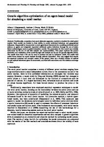
IV. EXAMPLE In this section, one numerical example is given to demonstrate GA-based identification of a nonlinear system with large time delays using a sparse Volterra filters. For the following example, the number of sampled points L is set to be 100, the number of chromosomes in each generation for GA is set to be 80, and the probability of mutation is set to be 0.01.

IEEE TRANSACTIONS ON SIGNAL PROCESSING, VOL. 47, NO. 12, DECEMBER 1999

3435

Fig. 2. Error convergence with and without forced mutation (SNR

Fig. 1. Error convergence for different SNR’s.

= 20 dB).

V. CONCLUSION Example: Assume that the nonlinear system to be modeled is y (k )

0 6) + 5 2 ( 0 6) + 3 4 0 4 3 ( 0 6) 0 2 5 2 ( 0 6) 3 + 3 5 ( 0 6) ( 0 7) + (

= 2u(k

u

k

u

: u(k

k

: u

k

: u

u(k

k

0 6) ( 0 7) 0 7) 0 3 4 ( 0 6) u k

u

k

n k)

u k

(14)

where the measurement noise n(1) is a random sequence uniformly distributed between 03 and 3, and the input signal u(1) is a random sequence uniformly distributed between 0R and R. The value of R is adjusted to obtain different SNR’s for the simulations. The associated linear vector equation as in (4) is given as y

= 2x 6 + 5x42 + 3:4x43

03

x 490

04

x 161

025

: x 162

+ 3:5x491 + n :

(15)

If a fourth-order Volterra filter with the number of delay taps N = 8 is used to model this nonlinear system, there are, in total, 494 Volterra kernels to be estimated. The GA with forced mutation is applied for the simulation. The convergence of the mean square error within 200 generations for SNR = 30, 20, 10, and 5 dB is simulated in Fig. 1. It is observed that the estimation converged within 200 generations. Taking the case that SNR = 20 dB as the example, the estimated linear vector equation is obtained as y ^

= 2:21x 6 + 0:44x35 + 5:31x42 + 3:61x43

0 2 88 0 0 08 0 2 98 :

x 162

:

x317

0 0 52 0 0 09

:

x 490

+ 3:95x 491 :

:

x 174

:

x 335

0 3 25 :

x 161

+ 0:02x190 + 0:33x225

0 0 05 :

x384

+ 0:19x399

(16)

The true kernel locations (underlined) are the locations corresponding to the Volterra kernels with magnitudes significantly greater than zero. In order to show the effect of forced mutation, GA’s with and without forced mutation were applied in the simulation. The square estimation error bound for GA to stop was set to be 30, which is the variance of the measurement noise. GA’s with and without forced simulation were applied 10 times, respectively, for SNR = 20 dB. On average, 68 and 564 generations were required to achieve the preset estimation error bound. It is obvious that the forced mutation did significantly improve the rate of convergence. With SNR = 20 dB, one of the typical error convergence for GA’s with and without forced mutation is compared in Fig. 2.

In this correspondence, the GA with a forced mutation operator was proposed for the kernel estimation of sparse Volterra filters. The GA was applied to search for the best set of kernel locations, whereas the least square error method was applied to estimate the associated Volterra kernels. It has been shown that the problem solved in this correspondence is essentially the combinatorial optimization problem. As the simple GA is applied to solve the problem of combinatorial optimization, it is possible that the solution set found by GA contains duplicated elements or the element out of range. The forced mutation operator was proposed to overcome these difficulties that usually arise in the combinatorial optimization. Since the linear finite impulse response (FIR) filter is a special case of a Volterra filter, the approach proposed here can be directly applied to the time delay estimation of a sparse FIR filter as well. ACKNOWLEDGMENT The author would like to thank the anonymous reviewers for their useful comments and suggestions, which helped improve the quality of this paper. REFERENCES [1] V. Z. Marmarelis, “Identification of nonlinear biological systems using Laguerre expansions of kernels,” Ann. Biomed. Eng., vol. 21, pp. 573–589, 1993. [2] R. D. Nowak and B. D. Van Veen, “Tensor product basis approximations for Volterra filters,” IEEE Trans. Signal Processing, vol. 44, pp. 36–50, Jan. 1996. [3] S. Benedetto and E. Biglieri, “Nonlinear equalization of digital satellite channels” IEEE J. Select. Areas Commun., vol. SAC-1, pp. 57–62, Jan. 1983. [4] O. Agazzi and D. G. Messerschmitt, “Nonlinear echo cancellation of data signals,” IEEE Trans. Commun., vol. COMM-30, pp. 2421–2433, Nov. 1982. [5] J. D. Taft, “Quadratic-linear filters for signal detection,” IEEE Trans. Signal Processing, vol. 39, pp. 2557–2559, 1991. [6] D. E. Goldberg, Genetic Algorithm in Search, Optimization, and Machine Learning. New York: Addison-Wesley, 1989. [7] L. Yao and W. A. Sethares, “Nonlinear parameter estimation via the genetic algorithm,” IEEE Trans. Signal Processing, vol. 42, pp. 927–935, Apr. 1994. [8] L. Yao, W. A. Sethares, and D. C. Kammer, “Sensor placement for on-orbit modal identification of large space structure via a genetic algorithm,” AIAA J., vol. 31, pp. 1922–1928, Oct. 1993. [9] L. L. Scharf, Statistical Signal Processing, Detection, Estimation, and Time Series Analysis. Reading, MA: Addison-Wesley, 1991. [10] G. Strang, Introduction to Linear Algebra. Wellesley, MA: WellesleyCambridge, 1993.