a genetic algorithm based bus scheduling model for transit network

Proceedings of the Eastern Asia Society for Transportation Studies, Vol. 5, pp. 477 - 489, 2005

A GENETIC ALGORITHM BASED BUS SCHEDULING MODEL FOR TRANSIT NETWORK Farhan Ahmad KIDWAI Lecturer Department of Civil Engineering University of Malaya 50603 Kuala Lumpur Malaysia Fax: +60-3-7967-5318 E-mail: [email protected]

Baldev Raj MARWAH Professor Department of Civil Engineering Indian Institute of Technology Kanpur - 208016 India Fax: +91-512-259-0007 E-mail: [email protected]

Kalyanmoy DEB Professor Department of Mech. Engineering Indian Institute of Technology Kanpur - 208016 India Fax: +91-512-259-0007 E-mail: [email protected]

Mohamed Rehan KARIM Professor Department of Civil Engineering University of Malaya 50603 Kuala Lumpur Malaysia Fax: +60-3-7967-5318 E-mail: [email protected]

Abstract: In this paper we present an optimization model for bus scheduling. This model constitutes one of the three major components of a solution approach for solving the transit network design problem. The problem of scheduling can be defined in the following general terms: Given the origin destination matrix for the bus trips for design period, the underlying bus network characterized by the overlapping routes, how optimally to allocate the buses among these routes? The bus scheduling problem is solved in two levels. In the first level, minimum frequency of buses required on each route, with the guarantee of load feasibility, is determined by considering each route individually. In the second level, the fleet size of first level is taken as upper bound and fleet size is again minimized by considering all routes together and using GAs. The model is applied to a real network, and results are presented. Key Words: Bus scheduling, Optimization, Genetic algorithms.

1. INTRODUCTION The design of bus transit system may be considered as a systematic decision process consisting of five stages: network design, frequency setting, time table development, bus scheduling and driver scheduling. However, the two most fundamental elements, namely, the design of routes and setting of frequencies, critically determine the system’s performance from both the operator and user point of view. Significant savings in resources can be made by reorganization of bus

477


routes and frequency to suit the actual travel demand. In Kidwai (1998) the solution framework for transit network design consists of three major components, namely, transit route design, transit assignment and transit scheduling. In this paper transit bus scheduling problem is formulated and solved in two phases. In the first phase, buses are assigned to individual routes by an interactive procedure. In the second phase, an attempt is made to further reduce the fleet size and genetic algorithms are used as an optimization tool. Genetic algorithms are search algorithms that are based on concepts of natural selection and natural genetics. The genetic algorithm method differs from other search methods in that it searches among a population of points and works with a coding of parameters, rather than the parameter value themselves. The transition scheme of the genetic algorithm is probabilistic, whereas traditional methods use gradient information. Finally the model is applied to a real network, and results are presented. 2. REVIEW OF PAST STUDIES A review of literature reveals various approaches and different computational tools for scheduling of urban bus transit problem. Lampkin and Saalmans (1967) formulated a constrained optimization problem for frequency determination. Their objective was to minimize the total travel time for a given fleet size constraint and a random search procedure was used for solution. Rea's (1972) model search for an optimum bus network by adjusting iteratively the frequencies and type of buses on each link to correspond to the link flow level, such that the service on some links is enhanced whilst on others it is depleted. The optimum situation is reached when no further change in link service levels is detected. Silman et al. (1974) determined optimum frequencies for a set of bus routes and fleet size, which could minimize the total travel time and discomfort (travelling without a seat) by a gradient method procedure. Hsu and Surti (1977) used the concept of marginal ridership (ridership provided by an additional unit of service frequency) to determine adequate frequency for each route for a given fleet size. Scheele (1977) proposed a mathematical programming algorithm of the compound minimization type for bus traffic model. The problem of optimal bus frequencies is solved by a gradient projection method. Dubois et al. (1979) used a two step procedure for frequency determination. Mandl (1979) assumed constant frequency on all the routes. Dhingra (1980) has developed a detailed simulation model for studying the effect of frequencies on various route level and network level measures of effectiveness. Furth and Wilson (1981) model allocates the available buses between time period and between routes so as to maximize net social benefit subject to constraints on total subsidy, fleet size and level of vehicle loading. Han and Wilson (1982) model recognizes passenger route choice behaviour and seeks to minimize a function of passenger wait time and bus crowding subject to constraints on number of buses available and the provision of enough capacity on each route. Baaj (1990) and Shih and Mahmassani (1994) have used the same model as Han and Wilson (1982), only their model differs in details of passenger path choice logic. Shih and Mahmassani (1994) have also used the concepts of optimal vehicle size, frequency adjustment for co-ordinated routes, timed transfer and transit centers. Dashora (1994) used an expert-system based model which allocates the buses to different routes between a maximum and minimum number, based on additional bus allocation factor (saving in waiting time/additional cost of operation) criteria. The candidate route for increasing a bus is the one for which additional bus allocation factor is maximum. The buses are allocated till fleet size is exhausted. Many researchers in the past decade have tried biologically motivated optimization techniques like

478


genetic algorithm and artificial neural network, for transit network design with promising results. Among them Xiong and Schneider (1993), Chakraborty et. al. (1995) Pattnaik et. al. (1998) Chien et. al. (2001), Khalage et. al. (2001), Bielli et. al. (2002), Tom and Mohan (2003) and Ngamchai and Lovell (2003), needs mention. 3. PROPOSED METHODOLOGY First general formulation for optimal bus allocation problem is given. In the present methodology a bi-level optimization is used to solve this problem. In the first level, minimum frequency of buses (then the number of buses) required on each route with the guarantee of load feasibility is determined by considering each route individually. Then by summing up the number of buses on each route fleet size is determined. In second level by taking the fleet size of first level as a lower bound, the fleet size is again minimized by considering all routes together and using GAs. 3.1 General Formulation In the present formulation, general model for bus scheduling problem is adopted similar to Han and Wilson (1982) and given as follows: Objective Minimize J = J (q ijk , fk, Ak) Subject to

Passenger flow assignment: q ijk = g ijk ( Vab, fr, Ar ) ∀ k ∈ SR, ij ∈ Lk, r ∈ Xij and a,b ∈ N Load feasibility: CAP × fk ≥ (q ijk )max ∀ k ∈ SR Fleet size:

∑

SR k =1

Tk × fk ≤ M

Where fk - frequency of buses operating on route k. Ak - set of other attributes associated with bus route k. CAP – capacity of buses operating on the network’s routes. q ijk - Passenger flow on link i – j of bus route k. g ijk - General function form which determines passenger flow assignment on link i – j of bus route k. Vab - origin destination flow between nodes a and b. N - set of nodes on the bus network. Lk - Set of links on bus route k. SR - set of bus routes. Tk - Round trip time of route k (including lay over time). Xij - Set of routes offering same service between nodes i and j. M – Total number of buses available. The objective function in the general case should include wait time and crowding levels for all passengers. Since many buses will be operating close to or at capacity on portions of their trips,

479


the specification of accurate wait time and crowding level function are extremely difficult (Han and Wilson, 1982). For this reason the simplified objective of minimizing the occupancy level at the most heavily loaded link on any route in the system is adopted here. This objective is different from, but related to minimizing wait times and crowding levels throughout the system, and is similar to the objective currently used by many operators in allocating buses in heavily utilized system. The load feasibility constraint requires that in a given period of time passengers should not be prevented from boarding a bus on their preferred route because inadequate capacity has been allocated to that route. This does not, of course, imply that every passenger will be able to board the first bus on that route because random fluctuation in the load will mean that some buses will be full at the heaviest points on each route. Some passengers who cannot board the first bus on their preferred route may, in fact, subsequently board an alternate route. Passenger path choice is based on an assumed flow assignment rule “Where there is one or more alternatives whose trip time is within a threshold of the minimum trip time a frequency share rule is applied”. This is an allocation formula that reflects the relative frequencies of service on alternative paths. 3.2 First Level Optimization The problem for first level optimization may be formulated as: Z=

∑

SR

( Tk × fk )

Objective

Minimize:

Subject to

Passenger flow assignment: q ijk = g ijk ( Vab, fr, Ar )

∀ k ∈ SR

Load feasibility: CAP × fk ≥ (q ijk )max

∀ k ∈ SR

k =1

The following algorithm is used to solve this problem. Step 1 For the given origin destination transit demand matrix and transit route network, assume the same number of trips on each route, n = 1; f nk . Step 2 Assign the origin destination transit demand matrix on the bus transit network using the assignment model discussed in next section. Step 3 For each route, find out the link carrying the maximum flow and determine the number of trips on each route using the formula.

f

n +1 k

=

( q ijk ) max 2 × bus capacity

These number of trips are rounded off to next higher integer. Step 4 If f nk +1 ∼ f nk is very small for all routes, go to Step 5; otherwise set n = n + 1 and go to Step 2. Step 5 Output the number of trips required on each route. Step 6 Find the number of buses required on each route to cater to these trips using the formula: f k × Tk Nk = time period Again these number of buses are rounded off to next higher integer. 480


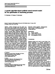
Step 7 Find the base fleet size (Wo) by summing up the number of buses on each route. Though there is no theoretical proof for convergence of the above algorithm, experience to date has indicated a converging pattern (Baaj, 1990; Han and Wilson, 1982). 3.3 Model for Transit Network Assignment The assignment model is crucial in transit network analysis because it determines the passenger flows on each links, which are used to calculate various costs and performance measures. This requires the assignment of passenger demand matrix to the set of routes that define any feasible transit network configuration. Han and Wilson (1982) used multi-path transit assignment, with transfer avoidance and/ or minimization acting as the primary choice criterion. Baaj and Mahmassani (1990) adopted this feature and developed a procedure for transit network analysis, and a similar procedure is adopted in the present study. 3.4 Second Level Optimization In the first level optimization, the base fleet size has been determined by considering individual route's capacity and no attempt is made to get the minimum fleet size on global bases (i.e. considering all the routes together). The reason why one can still reduce the fleet size below the base fleet size may be attributed to the extensive overlapping of the routes. If there is no overlapping of the routes, one can't hope to reduce the fleet size below the base value. Though there are various reasons of, how extensive overlapping of routes may help to reduce the fleet size, two reasons are discussed below. (a) In the routes shown in Figure 1 there is overlapping for many links. Suppose the links which carry the maximum flow (i.e. used for minimum number of bus determination in the first level of optimization) are (3) − (4) and (6) − (7) for routes RI and RII, respectively. If one bus is reduced on route RI, there will be violation of the load feasibility at link (3) − (4), but because this link is common with route RII and reserve capacity is available on this link as this link is not the maximum flow carrying link for route number RII, the extra demand of link (3) − (4) may be taken care of by buses on route RII. 1

11

RI

RII

2

3

4

12

5

6

7

8

13

14

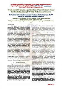
Figure 1. Example Network (b) Take the example of two overlapping routes shown in Figure 2. Here route RI is assumed to be much longer than route RII (which is quite possible as routes may vary in length from 5 to 15 km). The number of buses required on a route to make a fixed number of trips are directly proportional to the length (round trip time) of the route. It is further assumed that route RI is level optimization) are along the overlapping portion of the two routes. Then if two buses are reduced on route RI and one bus in increased on route RII, the number of trips on overlapping portion will remain the same and load feasibility constraint may not be violated even after one

481

Proceedings of the Eastern Asia Society for Transportation Studies, Vol. 5, pp. 477 - 489, 2005 RI 1

2

3

4

5

RII 21

6

7

8

23

22

9

10

11

12

24

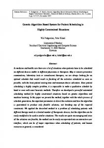
Figure 2. Example Network to Illustrate Bus Reduction bus is reduced below the base fleet size. These possibilities of reducing the base fleet size are investigated in the second level optimization using genetic algorithms (GAs). As GAs are not very common for transportation engineering applications, it is imperative at this stage to discuss their principles. 4. GENETIC ALGORITHMS The idea of genetic algorithms (GAs) was first conceived by Professor John Holland of the University of Michigan in 1975. Genetic algorithms are computer based search and optimization algorithms which work on the mechanics of natural genetics and natural selection (Goldberg, 1989). The mechanics of a simple genetic algorithm are simple involving copying strings and swapping partial strings. The explanation of why this simple process works is subtle yet powerful. Simplicity of operation and implicit parallelization are two of the main attractions of the genetic algorithm approach. 4.1 Working Principle GAs begin with a population of string structures created at random. Thereafter, each string in the population is evaluated. The population is then operated by three main operators - reproduction, crossovers and mutation - to create a hopefully better population. The population is further evaluated and tested for termination. If the termination criteria are not met, the population is again operated by above three operators and evaluated. This procedure is continued until the termination criteria are met. One cycle of these operators and the evaluation procedure is known as a generation in GA terminology. Figure 3 illustrates a pseudo code for a simple genetic algorithm. begin Initialize population of strings; Compute fitness of population; Repeat Reproduction; Crossover; Mutation; Compute fitness of population; Until (termination criteria); end. Figure 3. Pseudo Code for a Simple GA

482


4.2 Strings GA starts with initial population of strings. Each string represents all the problem variables in the optimization problem to be solved. These strings are created at random. These strings are similar to chromosomes in biological systems. The mechanism of genetic algorithms involves the manipulation of strings of 0 and 1. Since each string consists of binary digits, the coordinates of a point in a search space is influenced by the values of 1 or 0. The size of the string depends on the desired solution precision. The creation of strings in the initial population of GA is as simple as tossing an unbiased coin. The successive coin flips (head=l, tail=0) can be used to decide genes (bits) in a string. Then the next string is created. This process is continued till entire population of strings is created. 4.3 Coding and Decoding In order to use GA to solve the optimization problem, decision variables are first coded in some string structure, though this coding is not absolutely necessary. Binary coded strings having 1s and 0s are mostly used. The length of the string is usually determined according to the desired solution accuracy. Once the coding of the variables has been done, the corresponding point can be found using a fixed mapping rule, usually, the linear mapping rule is used (Goldberg, 1989). 4.4 Evaluation After all the values of variables are obtained, they can be used to calculate the objective function value. In general, a fitness function F(x) is first derived from the objective function and used in successive genetic operators. For maximization problems, the fitness function can be considered to be the same as the objective function i.e., F(x) = f(x). For minimization problems the fitness function is an equivalent maximization problem chosen such that the optimum point remains unchanged. The following fitness function is usually used (Goldberg, 1989). 1 F(x) = [1 + f ( x)] This transformation does not alter the location of the minima but converts a minimization problem to an equivalent maximization problem. The fitness function value of a string is known as the string's fitness. In the same way, all the fitness values of the strings in a particular generation are calculated. The maximum, minimum and average fitness values of the strings in a population are calculated. Then the termination criterion is checked. If the termination criterion is not reached, GA operators are applied to create a new population. 4.5 Genetic Algorithm Operators The population in GA is usually operated by three main operators: reproduction, crossover and mutation. These are applied to string population to create a new population. These operators involve random number generation, string copying, partial string exchanging and changing bits 0 to 1 and vice versa. These three operators are described below. Reproduction is usually the first operator applied on a population. Reproduction is a process in which individual strings are copied according to their fitness function values. Intuitively, we can think of the fitness function as some measure of profit, utility or goodness that we want to maximize. Copying strings according to their fitness values means that string with a higher value have a higher probability of contributing one or more offsprings in the next generation. A tournament size of two, known as binary tournament, is used in most applications and the same is used in the present study. After reproduction, crossover is applied to the string of the mating pool. It is intuitive from this

483


construction that good substrings from either parent string can be combined to form a better child string if appropriate site is chosen. Since the knowledge of an appropriate site is usually not known, a random site is chosen. But this random site selection is taken care of by selection (reproduction) operator, because if good strings are created by crossover, there will be more copies of them in the next mating pool, otherwise they will not survive beyond next generation. Crossover operator is mainly responsible for the search aspect of genetic algorithms; mutation operator is also used for this purpose sparingly. By mutation diversity can be maintained in the population, which helps in creating a better string. Mutation operator changes a 1 to a 0 and vice versa with a small mutation probability. The need for mutation is to keep diversity in the population. For example, if in a particular position along the string length all strings in the population have a value 0, and a 1 is needed in that location to obtain the optimum then neither reproduction nor crossover operator will be able to create a 1 in that location. The inclusion of mutation may turn that 0 into a 1. Furthermore, for local improvement of a solution and to avoid getting trapped in local optima, mutation may be found useful. One cycle of these operations and the subsequent evaluation procedure is known as one generation in GA terminology. 4.6 Termination Criteria When the average fitness of all the strings in a population is nearly equal to the best fitness, the population is said to have converged. When the population is converged, the GA is terminated. The same can be done by fixing maximum number of generations, the number of generations at which population will converge. In GA, maximum number of generations is generally used as the termination criteria. The same has been used in the present study. 5. PROBLEM FORMULATION FOR SECOND LEVEL OPTIMIZATION

As we know the number of buses on each route (Nk) from the first level optimization, it is sensible to make the search around these Nk values, in order to avoid otherwise a meaningless search. Therefore, a window is decided around the previously determined Nk values and search is made only in that window. In the present study, it is decided to search within a window of 8 buses around the previously determined Nk values. For example, if for a route k, value of Nk is 20 buses, then the search will be made only between 16 to 23 buses for this route. There is a rationale for selecting the window of 8 buses for search. In GA, variables are coded as binary strings and n bits are required for 2n different values of a variable. Therefore, one bit will be required for 2 buses, 2 bits for 4 buses, 3 bits for 8 buses and n bits for 2n buses. If we decide to take 2 bits for representing bus window of 4 on each route for searching an optima, it will give rise to a narrow search space and optima may lie outside this window. On the other hand if we decide to take 4 bits for representing bus window of 16 on each route to search for an optima, it will exponentially increase the search space and may give many infeasible (i.e. zero or negative buses on a route) values. After it is decided to use the window size of 8 buses, 3 bits will be required for each route. Therefore for k routes, a string of length 3 x k bits will be required. Because the window size is 8, the lower and upper limits on the number of buses for a route k will be, Nkmin = Nko - 4 Nkmax = Nko +3; respectively. Where Nko is the number of buses on route k from first level optimization. The problem for the

484


second level optimization may be stated as below. Objective

Minimize:

Z=

∑

SR k =1

Nk

Subject to Nkmin ≤

∑

SR k =1

Nk ≤ Nkmax

∀ k ∈ SR

Nk < W0

Passenger flow assignment Load feasibility: CAP × fk ≥ (q ijk )max

∀ k ∈ SR

Where, Nk - number of buses on route k, and W0 - Base fleet size (found in first level optimization). 6. GENETIC ALGORITHM FOR SOLUTION

In the above problem decision variables (number of buses on each route) can take only integer values and last two constraints are highly non-linear. Therefore, GAs which are best suited for such problems are used for solution. GA steps are given below. Step 1 Compute Nkmin values for each route as: Nkmin = Nko - 4. Step 2 Choose a selection operator, a crossover operator and a mutation operator. Choose population size, crossover probability and mutation probability. Choose a maximum allowable generation number. Step 3 In this step, GA creates an initial population of strings randomly. Based on the number of routes the required string length can be calculated. For example, if there are k routes, the string length should be k x 3. Step 4 In the fourth step, string is decoded and the actual bus number for each route are obtained using the formula, Nk = Nkmin+ decoded value of kth 3 bits of the string. For example, if there are three routes and Nkmin values for these routes are 6, 9 and 8, then for a typical string 110010101 the Nk values for the three routes will be 12 (6+6), 11 (9+2) and 13 (8+5), respectively; Step 5 Calculate the fleet size by summing up Nk values for all routes. If this fleet size is greater than or equal to the base fleet size, assign fitness a very small value; otherwise proceed with next step. Step 6 Compute frequencies using Nk values for each route. Assign the passengers on different links of the network using assignment model. Step 7 If the load feasibility constraint is violated, assign fitness a very small value; otherwise compute fitness using the formula C fitness = 1+ ∑ Nk where C is a constant used to normalize the objective function. Step 8 If the entire population of strings is processed, compute the best and average fitness value

485


in the generation and test for termination criteria; otherwise evaluate the next string in the population. Step 9 If the current generation is equal to the maximum number of generations assumed, the program is terminated and the scheduling giving the minimum fleet size is considered as the optimal schedule; otherwise the GA operators - reproduction, crossover and mutation are applied on the current population to obtain a new population of strings and the new population is processed again. 7. TESTING ON SAMPLE NETWORK

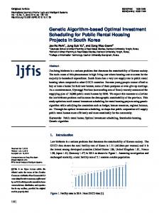
To test the proposed model, the road network of the city of Burdwan, West Bengal, India, with a total of 60 nodes and 70 links is selected as shown in Fig. 4. A conservative bus speed of 15 km/hour is assumed through out the network to convert the link distance in time units. A symmetric demand matrix for the design peak period of 3 hours is randomly generated to obtain 39 38

41

37

55

6 7

42 16

43

34

13

12 51

36

18

52

26 59

21

45

10

54 17

60

9

25

8 24

50 20

1

40

48 15

33

N

14

47

46 11

22

3

4 53

23

56 27

29

44 58

28 19

31 49

30

35

32 5 2

57

Figure 4. Road Network of Burdwan, W. Bengal, India test data. The route design algorithm (Kidwai, 1998) has produced 81 feasible solutions for different ranges of user and operator parameters, for the given road network and these solutions are used as an input for testing the scheduling model. Several external parameters which are required before running the numerical experiments are enumerated below.

486


• • • • • • •

Transfer penalty – 5 minutes of equivalent in-vehicle time. Bus capacity – 60 passengers. Minimum allowable frequency – 1 bus/hour. Number of buses on all routes – the number of buses on all routes which resulted from the first level optimization. Base fleet size – the fleet size produced by first level optimization. Bus search window size – a window size of 8 buses is used for making search around the number of buses determined in first level optimization, for all transit routes. GA parameters • String length – the string length required is 3 times the number of routes in a transit network. • Maximum number of generations – 100. • Population size – because string length is different for different runs of algorithm, therefore, population size is also varied according to the string length, the following ranges are fixed after preliminary testing. String length < 40 40 – 50 > 50 • • •

Population size 50 60 70

Cross over probability – 0.80, single point crossover is used. Mutation probability – 0.01, bitwise mutation is used. Binary tournament selection is used.

Out of the total 81 feasible solutions produced by transit route design algorithm, the scheduling model using GA reduced two buses below base fleet size for three transit networks and one bus for nine networks only. During the model formulation stage it was expected that GA based optimization will reduce the fleet size appreciably below the base fleet size. This meager reduction in base fleet size may be attributed due to very little overlapping of routes in the transit network the city of Burdwan. However, it is surmised that for transit networks with extensive overlapping the proposed algorithm would yield significant savings. 8. SUMMARY AND CONCLUSION

The optimal allocation of buses with a conventional approach poses considerable difficulties owing to the combinatorial nature of the problem and the complex nature of the route choice model. Hence genetic algorithms (GAs) are proposed as the computational tool because of their ability to handle large and complex problems. The solution framework for the present problem involves two phases: (1) allocation of buses on individual routes with maximum link flow as the criteria, and (2) further reduction of buses on network basis making use of genetic algorithms as an optimization tool. The proposed model, is applied to the transit network of the city of Burdwan, West Bengal, India. The reduction in fleet size is not significant using GA as it was expected during model formulation stage, the reason may be little overlapping of routes in test 487


network. It is recommended to test the model for dense transit networks with significant overlapping. The present study may also be extended by exploring the suitability of different GA parameters. REFERENCES

Baaj, M. H. (1990). The Transit Network Design Problem: An AI-Based Approach, Ph.D. thesis, Department of Civil Engineering, University of Texas, Austin, Texas. Baaj, M. H. and Mahmassani, H. S. (1990). TRUST: A Lisp Program for the Analysis of Transit Route Configuration, Transportation Research Record 1283, Transportation Research Board, Washington, D. C., pp 125 - 135. Bielli, M. , Caramia, M. and Carotenuto, P. (2002). Genetic algorithms in bus network optimization, Transportation Research Part C, Vol. 10, No.1, pp 19 - 34. Chakroborty, P. , Deb, K. and Subrahmanyam, .P. S. (1995). Optimal Scheduling of Urban Transit Systems Using Genetic Algorithms, ASCE Journal of Transportation Engineering, Vol. 121, No.6, pp 544-553. Chien, S., Yang, Z. and Hou E. (2001).Genetic algorithm approach for transit route planning and design, ASCE Journal of Transportation Engineering, Vol. 127, No.3, pp 200-207. Dashora, M. (1994). Development of an Expert System for Routing and Scheduling of Urban Bus Services, Ph.D. thesis, Department of Civil Engineering, lIT Bombay, INDIA. Dhingra, S. L. (1980). Simulation of Routing and Scheduling of City Bus Transit Network, Ph.D. thesis, Department of Civil Engineering, lIT Kanpur, INDIA. Dubois, D., Bell, G. and Llibre, M. (1979). A Set of Methods in Transportation Network Synthesis and Analysis, Journal of Operations Research Society, Vol. 30, No.9, pp 797-808. Furth, P. G. and Wilson, N. M. H.(1981). Setting Frequencies on B-us Routes: Theory and Practice, Transportation Research Record 818, Transportation Research Board, Washington, D. C., pp 1 - 7. Goldberg, D. E. (1989). Genetic Algorithms in Search, Optimization, and Machine Learning, Addison-Wesley Publishing Company, Inc., Mass., USA Han, A. F and Wilson, N. M. H (1982). The Allocation of Buses in Heavily Utilized Networks With Overlapping Routes, Transportation Research B, Vol. 16, No.3, pp 221 -232. Hsu, J. and Surti, V. H. (1977). Decomposition Approach to Bus Network Design, ASCE Journal of Transportation Engineering, Vol. 103, pp 447-459. Kalaga, R. K., Dutta, R. N. and Reddy, K.S. (2001). Allocation of buses on interdependent 488


regional bus transit routes, ASCE Journal of Transportation Engineering, Vol. 127, No.3, pp 208-214. Kidwai, F. A. (1998). Optimal Design of Bus Transit Network: A Genetic Algorithm Based Approach, Ph.D. thesis, Department of Civil Engineering, Indian Institute of Technology, Kanpur, India. Lampkin, W. and Saalmans, P. D. (1967). The Design of Routes, Service Frequencies and Schedules for a Municipal Bus Undertaking: A Case Study, Operation Research Quarterly 18, pp 375 - 397. Mandl, C. E. (1979). Evaluation and Optimization of Urban Public Transportation Networks, Presented at the Third European Congress on Operations Research, Amsterdam, Netherlands. Ngamchai, S. and Lovell D. J. (2003).Optimal time transfer in bus transit route network design using a genetic algorithm, ASCE Journal of Transportation Engineering, Vol. 129, No.5, pp 510-521. Newell, C. E. (1979). Some Issues Related to the Optimal Design of Bus Routes,Transportation Science 13 , pp 20 - 35. Patnaik, S. B., Mohan, S. and Tom, V.M. (1998). Urban Bus Transit Route Network Design Using Genetic Algorithms, ASCE Journal of Transportation Engineering, Vol. 124, No.4, pp 368-375. Rea, J. C. (1972).Designing Urban Transit Systems: An Approach to the Route Technology Selection Problem, Highway Research Record 417, Highway Research Board, Washington, D. C., pp 48 - 58. Scheele, S. (1977). A Mathematical Programming Algorithm for Optimal Bus Frequencies, Ph.D. thesis, Department of Mathematics, Linkoping University, Linkoping, Sweden Shih, M. and Mahmassani, H. S. (1994). A Design Methodology for Bus Transit Networks with Coordinated Operations, Research Report 60016-1,Center for Transportation Research, University of Texas at Austin, Austin, Texas. Silman, L. A., Barzily,Z. and Passy, U. (1974).Planning the Route System for Urban Buses, Computers and Operations Research, Vol. 1, pp 201 - 211. Tom, V. M. and Mohan, S. (2003). Transit Route Network Design Using Frequency Coded Genetic Algorithms, ASCE Journal of Transportation Engineering, Vol. 129, No.2, pp 186195. Xiong, Y. and Schneider, J. B. (1992).Transportation network design using a cumulative genetic algorithm and neural network, Transportation Research Record 1364, Transportation Research Board, Washington, D. C., pp 37 - 44.

489