Genetic Algorithm-Based Solver for Very Large Multiple Jigsaw Puzzles of Unknown Dimensions and Piece Orientation Dror Sholomon
Omid E. David
Dept. of Computer Science Bar-Ilan University Ramat-Gan 52900, Israel
Dept. of Computer Science Bar-Ilan University Ramat-Gan 52900, Israel
[email protected]
[email protected]
ABSTRACT In this paper we propose the first genetic algorithm (GA)based solver for jigsaw puzzles of unknown puzzle dimensions and unknown piece location and orientation. Our solver uses a novel crossover technique, and sets a new stateof-the-art in terms of the puzzle sizes solved and the accuracy obtained. The results are significantly improved, even when compared to previous solvers assuming known puzzle dimensions. Moreover, the solver successfully contends with a mixed bag of multiple puzzle pieces, assembling simultaneously all puzzles.
Categories and Subject Descriptors I.2.10 [Artificial Intelligence]: Vision and Scene Understanding
General Terms Algorithms
Keywords Computer Vision, Genetic Algorithms, Jigsaw Puzzle, Recombination Operators
1.
INTRODUCTION
Jigsaw puzzles are a popular form of entertainment, first produced around 1760 by John Spilsbury, a Londonian engraver and mapmaker. Given n different non-overlapping tiles of an image, the objective is to reconstruct the original image, taking advantage of both the shape and chromatic information of each piece. Despite the popularity and vast ∗Nathan Netanyahu is also with the Center for Automation Research, University of Maryland, College Park, MD 20742 (e-mail:
[email protected]). Permission to make digital or hard copies of all or part of this work for personal or classroom use is granted without fee provided that copies are not made or distributed for profit or commercial advantage and that copies bear this notice and the full citation on the first page. Copyrights for components of this work owned by others than ACM must be honored. Abstracting with credit is permitted. To copy otherwise, or republish, to post on servers or to redistribute to lists, requires prior specific permission and/or a fee. Request permissions from
[email protected]. GECCO’14, July 12–16, 2014, Vancouver, BC, Canada. Copyright 2014 ACM 978-1-4503-2662-9/14/07 ...$15.00. http://dx.doi.org/10.1145/2576768.2598289.
∗
Nathan S. Netanyahu
Dept. of Computer Science Bar-Ilan University Ramat-Gan 52900, Israel
[email protected]
distribution of jigsaw puzzles, their assembly is not trivial computationally, as this problem was proven to be NPhard [1, 7]. Nevertheless, a computational jigsaw solver may have applications in many real-world applications, such as biology [14], chemistry [20], literature [16], speech descrambling [22], archeology [2, 12], image editing [5], and the recovery of shredded documents or photographs [3, 15, 11, 6]. Regardless, as noted in [10], research of the topic may be justified solely due to its intriguing nature. Most recently proposed solvers employ greedy strategies. Greedy algorithms are known to be problematic when encountering local optima. Moreover, such solvers rarely offer a backtrack option, i.e., a possibility to cancel a piece assignment which seemed correct at first but then turned to be globally incorrect. Hence, state-of-the-art solvers are very successful on some images, but perform poorly on others. The enormous search space of the problem, containing many local optima, seems most suitable for a genetic algorithm (GA)-based solver. The use of genetic algorithms in the field was first attempted in 2002 by Toyama et al. [19] but its successful performance was limited to 64-piece puzzles, probably due to the inherent difficulty in designing a crossover operator for the problem [18]. More recently, Sholomon et al. [18] presented another GA-based solver which can handle up to 22,755-piece puzzles. Nevertheless, their solver can handle only puzzles with (1) known piece orientations, (2) known image dimensions, and (3) pieces of a single image. In this work we propose a novel GA-based solver, relaxing most previous assumptions. First, we assume no a priori knowledge regarding piece location or orientation. Second, we assume that the image dimensions (i.e., the number of row and column tiles) are unknown. Finally, we allow the input piece set to contain pieces from either a single image or from multiple images. In the case of a “mixed-bag” puzzle, the solver concurrently solves all puzzles, unmixing their pieces along the process. We set a new state-of-the-art by solving the largest and most complex puzzle ever (i.e., 22,755 pieces, which is twice the size of the current state-of-the-art without making any assumptions) and achieving the highest accuracy ever reported, even with respect to solvers that assume known image dimensions.
2.
RELATED WORK
Freeman and Garder [8] were the first to tackle computationally the jigsaw problem, in 1964. Their solver handled up to 9-piece puzzles, using only piece shape. Kosiba
(a)
(b)
(d)
(c)
(e)
Figure 1: Example of a relative relation assignment: (a) Pieces 4 and 7, (b)–(e) all possible image configurations of assigning the relative relation (4.b, 7.c). Note that the two pieces are always in the same relative configuration despite the different orientations.
et al. [13] were the first to facilitate the use of image content. Subsequent research has been confined to color-based square-piece puzzles, instead of the earlier shape-based variants. Cho et al. [4] presented a probabilistic puzzle solver that can handle up to 432 pieces, given some a priori knowledge of the puzzle (e.g., anchor pieces). Their results were improved a year later by Yang et al. [21], who presented a so-called particle filter-based solver. A major contribution to the field was made recently by Pomeranz et al. [17] who introduced, for the first time, a fully automated jigsaw puzzle solver that can handle square-piece puzzles of up to 3,000 pieces, without a priori knowledge of the image. Their solver treats puzzles with unknown piece location but with known orientation. Gallagher [9] was the first to handle puzzles with both unknown piece location and orientation, i.e., each piece might be misplaced and/or rotated by 90, 180 or 270 degrees. The latter solver was tested on 432- and 1,064piece puzzles and a single 9,600-piece image. Sholomon et al. [18] successfully solved a 22,755-piece puzzle with only piece location unknown. Thus, as far as we know, current state-of-the-art algorithms can solve correctly a 22,755-piece puzzle with unknown piece location and a 9,600-piece puzzle with unknown piece location and orientation. All of the above solvers make use of the image dimensions during the solution process. We believe our work provides for the first time a solver capable of perfectly reconstructing a 22,755piece puzzle with unknown piece location and orientation and no knowledge of the original image dimensions.
3.
PUZZLE SOLVING
In its most basic form, every puzzle solver requires an estimation function to evaluate the compatibility of adjacent pieces and a strategy for placing the pieces (as accurately as possible). We propose using genetic algorithms as a piece placement strategy, aimed at achieving an optimal global score with respect to compatibilities of adjacent
(a) Original Image
(b) Chromosome
Figure 2: Characteristics sought by crossover; chromosome shown correctly assembled a number of puzzle segments, most of which are incorrectly located (with respect to correct absolute location) or oriented (notice tower orientation versus flags); crossover operator should exploit correctly assembled segments and allow them to be translated and rotated in a child chromosome.
pieces in the resulting image. The proposed GA elements (e.g., chromosome representation, crossover operator, and fitness function) are required to tackle several non-trivial issues. First, the eventual solution needs to be valid, i.e., every puzzle piece should appear once and only once, without missing and/or duplicate pieces. Second, the resulting image dimensions should strive to meet those of the (unknown) dimensions of the original image, avoid undesirable cases (e.g., pseudo-linear configurations) which contrive to be optimal solutions. Third, in the spirit of a gradual, evolutionary improvement over time, puzzle segments assembled correctly, up to an exact location and orientation, should be tracked, inherited to child chromosomes, and undergo proper translation and rotation (see Figure 2).
(a)
(b) 1.b – 2.d
(c) 4.d – 8.c
(d) 8.d – 7.c
(e) 3.a – 4.c
(f) 2.c – 7.a
(g) 2.a – 6.b
(h) 5.b – 1.a
Figure 3: Different types of relative relation assignment; each sub-caption describes the corresponding assignment made, also marked by a red line, (c) rotation of pieces, (e) explicit assignment (4.c, 3.a) leading to an implicit assignment (3.d, 7.d), and (f) merge of two piece groups, during which the entire left group is rotated. Note how in (d) the assignment (2.a, 4.c) is geometrically infeasible due to a collision between pieces 1 and 7.
3.1
Chromosome Representation
We propose for each chromosome to be equivalent to a complete solution of the jigsaw puzzle problem, i.e., a suggested placement of all the pieces. Since the image dimensions are unknown, it is not clear how to store a piece configuration in a two-dimensional array (according to piece locations and orientations), in accordance with the actual image. Instead, we store, for each chromosome, only the relative placement of neighboring pieces. Since a piece orientation is unknown, for each given piece we denote its edges as a, b, c, d, starting clockwise from a random edge. To denote the relative placement of two pieces we may say, for example, that edge pi .b (i.e., edge b of piece pi ) is placed next to edge pj .c, thus encoding both the relative spatial location and orientation of the pieces. Figure 1 depicts the labeling of piece edges and their relative placement. Each chromosome is represented by an (n × 4) matrix (i.e., a matrix whose dimensions are the number of pieces times the number of piece edges), where a matrix entry xi,j (i = 1..n, j = 1..4) is the corresponding piece edge adjacent to xi .j (e.g., xi .j = p2 .c) or “none”, if no edge is placed next to it (e.g., at the puzzle’s boundary). This representation lends itself more easily to subsequent relative-placement evaluations and crossover operations.
3.2
Chromosome Evaluation
We use the dissimilarity measure below, which was presented in various previous works [17, 4, 18]. This measure relies on the premise that adjacent jigsaw pieces in the original image tend to share similar colors along their abutting edges, and thus, the sum (over all neighboring pixels) of squared color differences (over all color bands) should be minimal. Assuming that pieces pi , pj are represented in normalized L*a*b* space by a K × K × 3 matrix, where K is the height/width of a piece (in pixels), their dissimilarity, where pj is “to the right” of pi , for example, is v uK 3 uX X (xi (k, K, ch) − xj (k, 1, ch))2 . D(xi .b, xj .d) = t k=1 ch=1
(1)
when ch denotes a spectral channel. Obviously, to maximize the compatibility of two pieces, their dissimilarity should be minimized. We compute the compatibility of all possible edges for all possible pieces, summing up to 16 edges per piece pair. Notice that computing the dissimilarity between piece edges (e.g., between p1 .b and p2 .c) is invariant to their final piece rotation. For example, assume b is the right edge of piece p1 and c is the left edge of piece p2 , with respect to some initial piece orientation. The compatibility of p1 .b to p2 .c is similar whether or not the pieces are rotated, i.e., p2 is to the right of p1 (if the pieces are not rotated), or p2 is below p1 if they are rotated (clockwise) by 90 degrees. In any event, the final chromosome fitness is the sum of pairwise dissimilarities over all adjacent edges. Representing a chromosome, as suggested, by an (n × 4) matrix, where a matrix entry xi,j (i = 1..n, j = 1..4) corresponds to a single piece edge, we define its fitness as: 4 n X X
D(pi .j, xi,j )
(2)
i=1 j=1
where D is the dissimilarity of the two given edges (edge j of piece pi and the edge located at xi,j ). This value should, of course, be minimized. Special care should be taken in the case of xi,j = none, i.e., a piece edge with no adjacent pieces. Intuitively, “none” piece edges should be highly discouraged. In principle, only boundary pieces of the original image should contain none edges. Most boundary pieces should have only a single none edge, whereas the four corner pieces are expected to have two none edges each. (Ideally, no piece should have more than two none edges.) Assigning a dissimilarity of “0” to a none edge might cause the GA to converge to a non-rectangular image. On the other hand, assigning an extremely high value might lead to cases where image shape might take precedence over image content. Having tested the algorithm with many different values, we picked the dissimilarity of a none edge (i.e., D(pi .j, none)) to be twice the average of all dissimilarities (i.e., the average of all 16 pairwise dissimilarities over all piece pairs). It appears that this measure highly encourages the GA to reach a correct reconstruction of the
(a) Generation 1
(d) Generation 4
(b) Generation 2
(c) Generation 3
(e) Generation 5
(f) Final Generation (100)
Figure 4: Solution process of a 22,755-piece puzzle (largest puzzle solved with unknown piece orientation and image dimensions): (a)–(e) Best chromosomes achieved by the GA in the first to fifth generation, and (f) final generation. Note that every chromosome (image) contains all puzzle tiles, so its image results in varying dimensions (down scaled, for display purposes). The original image was perfectly reconstructed.
original image, with respect to both image dimensions and content.
3.3
Crossover Operator
The most involved element of the proposed GA is the crossover operator. Considering the proposed representation and in light of the chosen fitness function, one can grasp the major role undertaken by the crossover operator. The operator must verify the validity of each newly created chromosome. Traditionally, this means that each puzzle piece appears once and only once in the child chromosome, and no piece is missing or duplicated. The inherent difficulty surrounding merely this condition is likely to have delayed the derivation of an effective GA-based solver for the problem. Meeting this condition still assures no validity. Since chromosomes contain only relative relations (e.g., edge p1 .b is adjacent to edge p2 .c), the operator must also verify that all relative relation assignments result in a geometrically feasible image, i.e., that all pieces must be placed properly with no overlaps. Moreover, the operator should verify that all prospective characteristics (e.g., correctly assembled puzzle segments) discovered by the parents may be inherited by their offsprings, and allow these segments to be translated in space and rotated inside the offspring (see, e.g., Figure 2). We propose a novel specialized crossover operator to address the aforementioned challenges. In contrast to previous works and in accordance with the chosen representation, this operator is based on relative relations of pieces edges. The assignment of a relative relation, e.g., “edge p1 .b is adjacent to edge p2 .c”, is the basic building block of the operator. An example of such an assignment can be viewed in Figure 1. To maintain consistency, each assignment is double since it immediately implies the commutative relation (i.e., that edge p2 .c is adjacent to edge p1 .b). Each crossover consists of exactly n − 1 double relative relation assignments, resulting in a single connected component (albeit not necessarily rectangular). Examples of such images can be viewed
in Figure 4. (Note that since every chromosome contains all the puzzle pieces, its image results in varying dimensions. This is not depicted, as the figure is down scaled for display purposes.) The following paragraphs describe the complete crossover procedure. First, we describe the intrinsics of the relative relation assignment and then provide the full details of creating a child chromosome.
3.3.1
The Relative Relation Assignment
The crossover procedure starts with no relative relations; each puzzle piece is detached and isolated from the others. Each assignment of a relative relation between two piece edges falls inside one of three possible scenarios. The first option is for the relation to be between two detached pieces. Naturally, this is always the case of the first assignment. The double relation between the two edges is recorded and the pieces are inserted into a newly created “piece group”. Each such group is recorded inside a matrix, tracking the spatial relations of its pieces and verifying the geometrical validity of the represented sub-image. The second possible scenario is that one of the edges belongs to such a piece group, while the other is of a detached piece. Again, the relation is recorded and the detached piece is inserted, at the correct location, into the already existing group. Notice that by inserting a piece inside a group, implicit relations might be set, e.g., inserting a piece to the left of a piece results in it being inserted below another piece, as depicted in Figure 3. All such implicit relations are recorded at the end of the crossover operation. Unlike the first two cases, the third case requires extra care. This is the case of the two edges originating from two different piece groups. Notice that setting a relation between two edges belonging to the same group is prohibited, since it is either redundant (the pieces already conform implicitly to the relation) or results in an invalid image. The two piece groups should then be merged to a single connected component. Unfortunately, as can be seen in Figure 5, some piece
patible edges in a random order. Finally, we try to assign two random edges until completing n − 1 successful assignments. Upon termination, after merging all piece groups, the crossover results in a single matrix, containing all n − 1 pieces. The matrix records the absolute location and orientation of each piece in the resulting image. As mentioned earlier, the operator now scans the matrix, and records all relative relations created, both explicitly and implicitly, to the new chromosome. Note that this chromosome represents a geometrically valid images, containing each puzzle piece exactly once.
(a) Valid assignment
Until (n − 1) relative relations are assigned do (b) Geometrically infeasible assignment
1. Try assigning all common relative relations. 2. Try assigning all best-buddy relative relations.
Figure 5: Geometrically valid and invalid relative relation assignments. formations cannot be merged. The operator tries to merge the smaller group to the larger one, starting from the requested edge and continuing with all other recorded relations in the group. If a collision occurs between two pieces, the entire assignment of this particular relative relation is deemed illegal and is discarded, leaving the two groups disjoint. In case of a success, the new double relation is recorded and the two groups are merged into a single group. Notice that such a merge might change the orientation of all pieces inside the group being merged.
3.3.2
A Multi-Phased Algorithm
Having described the relative relation assignment, we now proceed with the assignment selection algorithm. Given two parent chromosomes, the operator initiates a multi-phased algorithm, described in Figure 6. Note that the algorithm continuously attempts to assign edges, until n − 1 successful assignments are made. Each assignment could fail if one of the edges has already been assigned during the above group merging; otherwise, it could fail as a result of the mutation process, with some low probability. The algorithm first tries to assign all common relations, i.e., all relative relations appearing in both parents. Second, the algorithm tries to assign relations which appear in at least one of the parents and are also best buddies. To understand this phase, we briefly review the concept of a best-buddy piece, first introduced by Pomeranz et al. [17]. Two pieces are said to be best buddies if each piece considers the other as its most compatible piece, according to the dissimilarity score. We generalize this notion for piece edges, i.e., two edges are considered best-buddy edges if each edge considers the other as its most compatible edge out of all existing edges. The edges xi .a and xj .d are said to best buddies if ∀ek ∈ Edges, D(xi .a, xj .d) ≤ D(xi .a, ek ) and ∀ep ∈ Edges, D(xj .d, xi .a) ≤ D(xj .d, ep )
(3)
where Edges is the set of all piece edges (i.e., sides a, b, c, and d of all n given pieces). Next, we introduce a greedy element. We compute, in advance, the most compatible edge for each of the 4 × n edges and then try to assign most com-
3. Try assigning all most-compatible relative relations. 4. Try assigning random relative relations.
Figure 6: Crossover overview
3.4
Rationale
The proposed genetic algorithm is based entirely on the concept of assigning relative relations between piece edges. This concept stems from the intuitive understanding that some puzzle segments are “easier” than others. A human solver will usually assemble first disjoint but distinct elements (e.g., animals, humans, vehicles, etc.), gradually joining them together. The assembly of more difficult parts (skies, sea, woods, and other background scenes) would be deferred to a later stage, when there are less pieces to choose from, which makes each decision easier. We mimic this behavior by allowing the solver to concurrently assemble different puzzle segments (piece groups), forcing it to merge them only at later stages. This advantage should be constructive especially in the case of puzzle pieces belonging to multiple images (i.e., a “mixed bag” of pieces), as the solver may handle each sub-image separately, as opposed to tackling the entire image of multiple excessive pieces. Correctly assembled segments in the parents are identified either by their mutual appearance in both parents, or by a greedy consideration (due to a very high compatibility of certain edges). Only the relative relation between the edges is inherited, as the segments might be easily rotated and translated in space during the crossover procedure.
3.5
GA Parameters
We use the standard roulette-wheel selection. In each generation we start by copying the best four chromosomes. The following are the parameters used: population size = 300 number of generations = 100 probability of not using a shared relation = 0.001
(a) Generation 1
(d) Generation 4
(b) Generation 2
(c) Generation 3
(e) Generation 5
(f) Final Generation (100)
Figure 7: Solution process of a “mixed-bag” puzzle, composed of four different 432-piece puzzles: (a)–(e) Best chromosomes achieved by the GA from first to fifth generation, and (f) final generation. All original four images were perfectly reconstructed. GA has no knowledge that given pieces belong to different images. # Pieces 432 540 805 5,015 10,375
Neighbor 94.88% 94.08% 94.12% 94.90% 98.03%
Perfect 11 8 6 7 4
Table 1: Accuracy results under neighbor comparison on different benchmark sets. For each set we report the average accuracy obtained by the GA and number of puzzles perfectly reconstructed (out of 20).
4.
RESULTS
To evaluate the accuracy results of each assembled image, we adopt the neighbor comparison measure used in all previous works, i.e., the fraction of correct pairwise piece adjacencies (with respect to the original image). In all experiments we used a standard tile size of 28 × 28 pixels. We tested our solver against previously published benchmark sets [17, 18, 4] containing 20-image sets of 432-, 540-, 805-, 5,015-, and 10,375-piece puzzles. We report in Table 1 the average accuracy results per set, as well as the number of puzzles reconstructed perfectly. The results obtained for the set of 432-piece puzzles can be compared to the ones achieved by [9] on the same image set (see Table 2). We stress that the solver in [9] assumes known image dimensions to improve the accuracy results (described there as the “trimming” and “filling” stages), while ours does not. According to Table 6 in [9], their algorithm results in an average of 90.4%, i.e., we achieve a significant improvement of over 4% with less assumptions. The largest puzzle that has been attempted so far with pieces of unknown orientation is a 9,600-piece puzzle. We attempted a 22,755-piece puzzle (i.e., more than twice larger), with unknown piece orientation and unknown image dimensions. As can be seen in Figure 4, perfect reconstruction was achieved. The solution process required a meager 3.5 hours
Gallagher [9] GA
Neighbor 90.4% 94.88%
Perfect 9 11
Table 2: Performance comparison for puzzles with 432 pieces. Note that [9] assumes known image dimensions to improve accuracy results, while our solver does not.
on a modern PC (compared to 23.5 hours reported in [9] for the 9,600 piece-puzzle). Finally, we applied the solver to “mixed-bag” puzzles, i.e., puzzles containing pieces from multiple images. Of course, the solver is unaware of the image dimensions, and of the fact that multiple images are involved. We created a mixed puzzle by combining four different 432-piece puzzles. Figure 7 depicts the gradual assembly of the puzzle until a perfect reconstruction of all four images is achieved. Next, we created another mixed puzzle by combining 16,405 pieces from seven different images; three 5,015-piece puzzles and four smaller ones. To the best of our knowledge, this is the most complex mixed-bag that has been solved, in terms of both the puzzle size and the number of mixed images. Despite containing a much larger number of pieces (relatively to single-image puzzles solved previously), the GA succeeds in fully reconstructing all the seven puzzles. Figure 8 shows the reassembled puzzles.
5.
CONCLUSIONS
In this paper we presented, for the first time, a GA-based solver capable of handling puzzles with (1) pieces of unknown orientation, (2) unknown image dimensions, and (3) pieces originating from multiple images. Our solver sets a new state-of-the-art in terms of the accuracy achieved and the complexity of the puzzles handled. We improved significantly results obtained by previous works, making almost no assumptions. Specifically, we successfully tackled puzzles of more than twice the size that has been attempted before
(a)
(b)
Figure 8: Perfect reconstruction of a “mixed-bag” puzzle. This puzzle is constructed of 16,405 pieces from seven different images; three 5,015-piece puzzles and four smaller puzzles. As far as we know, this is the largest and most complex mixed puzzle that has been solved, in terms of size and number of puzzles.
with the same relaxed assumptions [9]. Finally, we showed how to assemble mixed puzzles, i.e., puzzles with pieces from multiple different images. As far as we know, the mixed puzzle solved in this paper is the largest and most complex in terms of the total number of pieces and the number of mixed images.
6.
REFERENCES
[1] T. Altman. Solving the jigsaw puzzle problem in linear time. Applied Artificial Intelligence an International Journal, 3(4):453–462, 1989. [2] B. Brown, C. Toler-Franklin, D. Nehab, M. Burns, D. Dobkin, A. Vlachopoulos, C. Doumas, S. Rusinkiewicz, and T. Weyrich. A system for high-volume acquisition and matching of fresco fragments: Reassembling Theran wall paintings. ACM Transactions on Graphics, 27(3):84, 2008. [3] S. Cao, H. Liu, and S. Yan. Automated assembly of shredded pieces from multiple photos. In IEEE Int. Conf. on Multimedia and Expo, pages 358–363, 2010. [4] T. Cho, S. Avidan, and W. Freeman. A probabilistic image jigsaw puzzle solver. In IEEE Conference on Computer Vision and Pattern Recognition, pages 183–190, 2010. [5] T. Cho, M. Butman, S. Avidan, and W. Freeman. The patch transform and its applications to image editing. In IEEE Conference on Computer Vision and Pattern Recognition, pages 1–8, 2008. [6] A. Deever and A. Gallagher. Semi-automatic assembly of real cross-cut shredded documents. In International Conference on Image Processing, pages 233–236, 2012. [7] E. Demaine and M. Demaine. Jigsaw puzzles, edge matching, and polyomino packing: Connections and complexity. Graphs and Combinatorics, 23:195–208, 2007. [8] H. Freeman and L. Garder. Apictorial jigsaw puzzles: The computer solution of a problem in pattern recognition. IEEE Transactions on Electronic Computers, EC-13(2):118–127, 1964. [9] A. Gallagher. Jigsaw puzzles with pieces of unknown orientation. In IEEE Conference on Computer Vision and Pattern Recognition, pages 382–389, 2012. [10] D. Goldberg, C. Malon, and M. Bern. A global approach to automatic solution of jigsaw puzzles. Computational Geometry: Theory and Applications, 28(2-3):165–174, 2004.
[11] E. Justino, L. Oliveira, and C. Freitas. Reconstructing shredded documents through feature matching. Forensic Science International, 160(2):140–147, 2006. [12] D. Koller and M. Levoy. Computer-aided reconstruction and new matches in the forma urbis romae. Bullettino Della Commissione Archeologica Comunale di Roma, pages 103–125, 2006. [13] D. A. Kosiba, P. M. Devaux, S. Balasubramanian, T. L. Gandhi, and K. Kasturi. An automatic jigsaw puzzle solver. In International Conference on Pattern Recognition, volume 1, pages 616–618, 1994. [14] W. Marande and G. Burger. Mitochondrial DNA as a genomic jigsaw puzzle. Science, 318(5849):415–415, 2007. [15] M. Marques and C. Freitas. Reconstructing strip-shredded documents using color as feature matching. In ACM Symposium on Applied Computing, pages 893–894, 2009. [16] A. Q. Morton and M. Levison. The computer in literary studies. In IFIP Congress, pages 1072–1081, 1968. [17] D. Pomeranz, M. Shemesh, and O. Ben-Shahar. A fully automated greedy square jigsaw puzzle solver. In IEEE Conference on Computer Vision and Pattern Recognition, pages 9–16, 2011. [18] D. Sholomon, O. E. David, and N. S. Netanyahu. A genetic algorithm-based solver for very large jigsaw puzzles. In IEEE Conference on Computer Vision and Pattern Recognition, pages 1767–1774, 2013. [19] F. Toyama, Y. Fujiki, K. Shoji, and J. Miyamichi. Assembly of puzzles using a genetic algorithm. In IEEE Int. Conf. on Pattern Recognition, volume 4, pages 389–392, 2002. [20] C.-S. E. Wang. Determining molecular conformation from distance or density data. PhD thesis, Massachusetts Institute of Technology, Dept. of Electrical Engineering and Computer Science, 2000. [21] X. Yang, N. Adluru, and L. J. Latecki. Particle filter with state permutations for solving image jigsaw puzzles. In IEEE Conference on Computer Vision and Pattern Recognition, pages 2873–2880, 2011. [22] Y. Zhao, M. Su, Z. Chou, and J. Lee. A puzzle solver and its application in speech descrambling. In WSEAS International Conference on Computer Engineering and Applications, pages 171–176, 2007.