Geometric Collocation Method on SO (3) with Application to Optimal ...

Hindawi Publishing Corporation Mathematical Problems in Engineering Volume 2015, Article ID 790409, 14 pages http://dx.doi.org/10.1155/2015/790409

Research Article Geometric Collocation Method on SO(3) with Application to Optimal Attitude Control of a 3D Rotating Rigid Body Xiaojia Xiang, Lizhen Wu, Lincheng Shen, and Jie Li College of Mechatronic Engineering and Automation, National University of Defense Technology, Changsha, Hunan 410073, China Correspondence should be addressed to Jie Li; [email protected] Received 22 August 2015; Accepted 13 October 2015 Academic Editor: Naohisa Otsuka Copyright © 2015 Xiaojia Xiang et al. This is an open access article distributed under the Creative Commons Attribution License, which permits unrestricted use, distribution, and reproduction in any medium, provided the original work is properly cited. The collocation method is extended to the special orthogonal group SO(3) with application to optimal attitude control (OAC) of a rigid body. A left-invariant rigid-body attitude dynamical model on SO(3) is established. For the left invariance of the attitude configuration equation in body-fixed frame, a geometrically exact numerical method on SO(3), referred to as the geometric collocation method, is proposed by deriving the equivalent Lie algebra equation in so(3) of the left-invariant configuration equation. When compared with the general Gauss pseudo-spectral method, the explicit RKMK, and Lie group variational integrator having the same order and stepsize in numerical tests for evolving a free-floating rigid-body attitude dynamics, the proposed method is higher in accuracy, time performance, and structural conservativeness. In addition, the numerical method is applied to solve a constrained OAC problem on SO(3). The optimal control problem is transcribed into a nonlinear programming problem, in which the equivalent Lie algebra equation is being considered as the defect constraints instead of the configuration equation. The transcription method is coordinate-free and does not need chart switching or special handling of singularities. More importantly, with the numerical advantage of the geometric collocation method, the proposed OAC method may generate satisfying convergence rate.

1. Introduction Attitude control is one of the basic technologies that an object’s motioning relies on, and thus it has been the research focus in motion control technology. For object motion, to enhance its performance and security, it is required to save its energy consumption and advance control performance itself, and the new control methods continue to emerge. There is no doubt that optimal control theory is the most natural framework toward conformity with meeting the above requirements. However, except that the linear quadratic issues such simple question, analytical solutions are seldom available or even possible. As a result, more often than not, one resorts to numerical techniques. Numerical methods for solving optimal control problems are divided into two major classes [1]: indirect methods and direct methods. In an indirect method, the calculus of variations [2] and the Pontryagin maximum principle [3] are used to determine the first-order optimality conditions of the original optimal control problem, so, it converts the optimal control problem

to a two-point boundary-value problem, including indirect shooting method [4] and indirect multiple-shooting method [5]. The primary advantage of the indirect methods lies in their high accuracy and assurances that the solution satisfies the necessary optimality conditions. However, indirect methods also have significant disadvantages. First, the necessary optimality conditions must be derived analytically; for most problems this derivation is difficult; Second, the radius of convergence is typically small. Third, a guess for the costates must be provided. In a direct method, the state and/or control of the optimal control problem is discretized in some manner and the problem is transcribed into a nonlinear programming problem (NLP), and, then, the NLP is solved using wellknown optimization techniques, including direct shooting, collocation methods. Although not as high in precision as indirect methods, direct methods also have advantages because the optimality conditions do not need to be derived, and they have a large radius of convergence. In general, the attitude of an object is represented by the Euler angle. However, when the object is regarded as a single

2 rigid body in three-dimensional space, the configuration of its rotation actually constructs a special Lie group called the special orthogonal group SO(3) [6]. In recent years, some researchers have applied optimal control on a Lie group to attitude control of a 3D rotating rigid body, to reduce the computational burden, or to provide a coordinate-free approach to avoid expensive chart switching, special handling of singularities, and numerical drift [7, 8]. Bloch et al. [9] and Hussein et al. [10] study a discrete variational optimal control problem for the rigid body on SO(3), and they describe the dynamical equations of the mechanical system as a geometric structure-preserving model referred to as a Lie group variational integrator and then use Lagrange’s method to derive the discrete necessary conditions (i.e., two-point boundary-value problem) which are solved by a standard nonlinear root-finding method. Lee et al. [7] propose an accurate computational approach for a nonconvex optimal attitude control (OAC) for a rigid body, in which the use of geometrically exact computations on SO(3) guarantees that the approach has excellent convergence properties. Similar to [7], the problem is also formulated directly as a discrete time optimization problem using a Lie group variational integrator; the discrete time necessary conditions for optimality are derived and solved by an efficient computational shooting method. Kobilarov and Marsden [11] extend the above conclusion to more general optimal control problems of mechanical systems on Lie groups and develop an efficient numerical method that exploits the structure of the state space and preserves the system motion invariants. The abovementioned works have some common features: first, instead of discretizing equations of motion, they all use a discrete variational integrator obtained from the discrete Lagranged’Alembert principle, a process that better approximates the equations of motion; second, they are all indirect optimal control methods. In this paper, we turn to direct methods to solve the OAC problem on SO(3). Among the direct methods, the collocation method, also known as a pseudo-spectral method, is widely used in rigid body attitude optimization (including UAV, satellite, space shuttle, launch vehicle, and supersonic aircraft) by virtue of its high accuracy and spectral (or exponential) convergence rate [1]. In the context of a Lie group, to our knowledge, Moulla et al. [12] are the first to propose the concept of the “geometric pseudo-spectral method.” They suggest a polynomial pseudo-spectral method that preserves the geometric structure of port-Hamiltonian systems, phenomenological laws, and conservation laws without introducing any uncontrolled numerical dissipation. However, their method is designed only for portHamiltonian systems in a special structure, which implies that the Dirac structure, therefore, could not be directly extended to the systems on SO(3). Thereby, how to apply the pseudo-spectral method to the OAC problem on SO(3) and conserve its geometric properties is still an open question, which is also the major topic studied in this paper. In this work, we study a constrained attitude control problem for the rigid body on SO(3) based on pseudo-spectral collocation method. First, we establish a left-invariant rigidbody attitude dynamical model in body-fixed frame on SO(3). Second, for the left invariance of attitude configuration

Mathematical Problems in Engineering in the body-fixed frame, we provide a discretization mechanism known as the geometric collocation method on SO(3), which may improve the accuracy of evolving trajectory and the convergence rate through applying different collocation strategies to the configuration equation and the velocity equation, respectively. For the configuration equation, since its geometric properties could not be preserved if the general pseudo-spectral method is directly applied to it, drawing on Engø’s idea about the equivariant map [13], we transform the configuration equation on SO(3) into an equivalent equation in the corresponding Lie algebra space [14] and then the solutions to the equivalent equation at discrete points are transformed into configuration at corresponding points via the coordinate map. For the velocity equation, we can use the general pseudo-spectral method directly to compute the velocities at the discrete points that are the same as those of configuration, since the velocity belongs to the Lie algebra space that is isomorphic to the Euclidean space. Under the condition that it has the same 4th order and large stepsize, the proposed method is compared with the general Gauss pseudo-spectral method [15], explicit RKMK [16], and Lie group variational integrator [7, 8]. We find that the accuracy of the proposed method is superior to other methods, except that the explicit RKMK demonstrates a higher convergence rate than the other methods. Furthermore, the method could preserve the structural characteristics of the Lie group precisely. Finally, we apply the above numerical method to a constrained OAC problem. In addition, the numerical method is used to solve the constrained OAC problem on SO(3). The optimal control problem is transcribed into a nonlinear programming problem, in which the equivalent Lie algebra equation is considered as the defect constraints instead of configuration equation. The transcription method is coordinate-free and does not need chart switching or special handling of singularities. More importantly, with the numerical advantage of the geometric collocation method, the OAC method exhibits a high convergence rate. The rest of this paper is organized as follows. Section 2 proposes a left-invariant rigid-body attitude dynamical model on SO(3). The geometric collocation method for the leftinvariant attitude dynamics system on SO(3) is given in Section 3, where Section 3.1 provides a general pseudo-spectral collocation method in the Euclidean space, Section 3.2 presents the Legendre-Gauss pseudo-spectral collocation method on SO(3), and, then, the corresponding algorithm is given in Section 3.3, and numerical tests are carried out on a free-floating rigid body model in comparison with four other numerical methods in Section 3.4. In Section 4, the proposed collocation is applied to a typical OAC problem and compared with several prior works. Finally, the conclusions and future work are outlined in Section 5.

2. Kinematics and Dynamics of Attitude Motion of a Rigid Body on SO(3) 2.1. Left-Invariant Mechanical System in a Body-Fixed Frame. The motion of a rigid body on Lie group 𝐺 could be described in a space frame or a body-fixed frame. To avoid confusion,

Mathematical Problems in Engineering

3

we would consider the motion of a single rigid body in a body-fixed frame in the sequel.

(LG-PC) method [1]. Take, for example, solving the following differential equation in R𝑛 at 𝑡𝑓 ,

Definition 1 (left-invariant mechanical systems on Lie group 𝐺 [6]). In a body-fixed frame, the motion of a rigid body could be described as a left-invariant mechanical system as follows: 𝑔̇ = 𝑇𝑒 𝐿 𝑔 ∘ 𝜉̂ ∈ 𝑇𝑔 𝐺,

∀𝑔 ∈ 𝐺,

𝑥̇ (𝑡)|𝑡 = 𝑓 (𝑡, 𝑥 (𝑡)) , 𝑥 (𝑡0 ) = 𝑥0 ∈ R𝑛 ,

(4) 𝑡0 ≤ 𝑡 ≤ 𝑡𝑓 .

(1)

where 𝑔 denotes the configuration of a rigid body in 𝐺 and 𝜉̂ = 𝑇𝑔−1 𝑔̇ ∈ 𝑇𝑒 𝐺 denotes the velocity of the rigid body in the body-fixed frame, where 𝑇𝑒 𝐺 fl g, known as the Lie algebra, is the tangent space at the identity 𝑒 of 𝐺 and “∧” is the hat operator satisfying isomorphism ̂∙ : R𝑛 → g with “∨” being its inverse mapping. 𝐿 𝑔 : 𝐺 → 𝐺 represents the left translation; that is, 𝐿 𝑔 (ℎ) = 𝑔ℎ, ∀ℎ ∈ 𝐺, and 𝑇𝑒 𝐿 𝑔 is its tangent space at 𝑒. For the matrix group, such as SO(3), ̂ “Left-invariant” SE(2), and SE(3), (1) is equivalent to 𝑔̇ = 𝑔⋅ 𝜉. implies that the mechanical system is invariant under left multiplication by constant matrices.

First, we equally divide a time interval [𝑡0 , 𝑡𝑓 ] into several time subintervals [𝑡𝑘 , 𝑡𝑘+1 ] with the stepsize being ℎ and transform the time interval 𝑡 ∈ [𝑡𝑘 , 𝑡𝑘+1 ] into 𝜏 ∈ [−1, 1] via the affine transformation 𝑡 = [(𝑡𝑘+1 − 𝑡𝑘 ) ⋅ 𝜏 + (𝑡𝑘+1 + 𝑡𝑘 )]/2. Thus, accordingly, (4) over [𝑡𝑘 , 𝑡𝑘+1 ] becomes 𝑥̇ (𝜏)|𝜏 =

𝑡𝑘+1 − 𝑡𝑘 𝑓 (𝜏, 𝑥 (𝜏)) , 2

− 1 ≤ 𝜏 ≤ 1.

Let 𝜏1 < ⋅ ⋅ ⋅ < 𝜏𝑁 be collocation points in [−1, 1] and 𝜏0 = −1. We approximate the solution of (5) by the following formula: 𝑁

𝑥 (𝜏) ≈ 𝑋 (𝜏) = ∑ 𝑥𝑖 ⋅ 𝐿 𝑖 (𝜏) , 2.2. Kinematics and Dynamics of Attitude Motion of a Rigid Body on SO(3). SO(3) is called the special orthogonal group, whose group element is the rotational component of the body-fixed frame {𝑏} relative to the space frame {𝑎} [6]. The left-invariant kinematics of attitude motion of a rigid body on SO(3) are given by 𝑏 𝑏 ̂𝑎𝑏 𝑅̇ 𝑎𝑏 (𝑡) = 𝑅𝑎𝑏 (𝑡) ⋅ 𝜔 (𝑡) fl 𝐺 (𝜔𝑎𝑏 (𝑡) , 𝑅𝑎𝑏 (𝑡)) ,

(2)

𝑏 where 𝑅𝑎𝑏 (𝑡) and 𝜔𝑎𝑏 (𝑡) denote the attitude configuration and angular velocity of a rotating rigid body on SO(3). The hat 𝑏 ̂𝑎𝑏 operator ̂∙ : R3 → so(3), for all 𝑦 ∈ R3 , satisfying 𝜔 (𝑡)⋅𝑦 = 𝑏 𝜔𝑎𝑏 (𝑡) × 𝑦, where × is vector cross product [6]. And it is known that the attitude dynamics of the rigid body are generally satisfying [10, 11]

(6)

𝑖=0

where 𝐿 𝑖 (𝜏) = ∏𝑁 𝑗=0,𝑗=𝑖̸ (𝜏 − 𝜏𝑗 )/(𝜏𝑖 − 𝜏𝑗 ) denotes Lagrange polynomials, satisfying the isolation property {1, 𝐿 𝑖 (𝑐𝑗 ) = 𝛿𝑖𝑗 = { 0, {

𝑖=𝑗 𝑖 ≠ 𝑗.

(7)

Equation (6) together with the isolation property leads to 𝑥𝑖 = 𝑥(𝜏𝑖 ), thereby 𝑋(𝜏𝑖 ) = 𝑥(𝜏𝑖 ). Through expressing the derivative of the Lagrange polynomials at the collocation points in differential matrix form 𝐷 = [𝑑𝑗𝑖 ] ∈ R𝑁×(𝑁+1) , where 𝑁

∏𝑁 𝑘=0,𝑘=𝑖,𝑙 ̸ (𝑐𝑗 − 𝑐𝑘 )

𝑙=0

∏𝑁 𝑘=0,𝑘=𝑖̸ (𝑐𝑖 − 𝑐𝑘 )

𝑑𝑗𝑖 = 𝐿̇ 𝑖 (𝑐𝑗 ) = ∑

𝑏 𝑏 𝑏 𝜔̇ 𝑎𝑏 (𝑡) = 𝐽−1 [𝐽𝜔𝑎𝑏 (𝑡) × 𝜔𝑎𝑏 (𝑡) ∗ + 𝑅𝑎𝑏 (𝑡) 𝜕𝑅𝑎𝑏 (𝑡) 𝑉 (𝑅𝑎𝑏 (𝑡)) + 𝑇ext (𝑡)]

(5)

,

(8)

𝑗 = 1, . . . , 𝑁, 𝑖 = 0, . . . , 𝑁, (3)

𝑏 fl 𝐹 (𝜔𝑎𝑏 (𝑡) , 𝑅𝑎𝑏 (𝑡) , 𝑇ext (𝑡)) ,

where 𝐽 is referred to as the inertia matrix of the rigid body, ∗ (𝑡)𝜕𝑅𝑎𝑏 (𝑡) 𝑉(𝑅𝑎𝑏 (𝑡)) denotes the moment of the conserva𝑅𝑎𝑏 tive force with 𝑉(𝑅𝑎𝑏 (𝑡)) being potential energy, and 𝑇ext (𝑡) fl 𝐵(𝑡) ⋅ 𝑢(𝑡) is that of the nonconservative external force with 𝐵(𝑡) being the control conjugate vector.

3. Legendre-Gauss Geometric Pseudo-Spectral Collocation Method on SO(3) 3.1. Legendre-Gauss Pseudo-Spectral Collocation Method in the Euclidean Space. Before collocating the left-invariant mechanical system on SO(3), we briefly describe the basic principle of the Legendre-Gauss pseudo-spectral collocation

we can write (5) at the collocation points as a set of differential algebra equations: 𝑁

∑𝑑𝑗𝑖 ⋅ 𝑋 (𝑐𝑖 ) = 𝑖=0

𝑡𝑘+1 − 𝑡𝑘 𝑓 (𝑐𝑗 , 𝑋 (𝑐𝑗 )) , 2

(9) 𝑗 = 1, . . . , 𝑁.

Based on the above equations, we establish the following defect equations, 𝑁

𝜍𝑗 = ∑𝑑𝑗𝑖 ⋅ 𝑋 (𝑐𝑖 ) − 𝑖=0

𝑡𝑘+1 − 𝑡𝑘 𝑓 (𝑐𝑗 , 𝑋 (𝑐𝑗 )) , 2

(10)

𝑗 = 1, . . . , 𝑁, and apply iterative algorithms to the above equations so as to determine the approximation to 𝑥(𝜏) at the collocation

4

Mathematical Problems in Engineering

points. Finally, according to the following formula, we obtain the approximation to (4) at the endpoint 𝑡𝑘+1 of time subinterval [𝑡𝑘 , 𝑡𝑘+1 ]: 𝑥 (𝑡𝑘+1 ) ≈ 𝑋 (𝑡𝑘 ) +

𝑡𝑘+1 − 𝑡𝑘 𝑁 ∑𝜛𝑗 ⋅ 𝑓 (𝑐𝑗 , 𝑋 (𝑐𝑗 )) , 2 𝑗=1

(11)

collocation method to solve the equivalent equation, and finally map its solution back to configuration space. As mentioned earlier, since the Lie algebra space is isomorphic to the Euclid space to which the attitudes dynamics belong, and before discretizing the configuration equation, we directly use the general pseudo-spectral method to collocate the angular velocities at the discrete points.

1

where 𝜛𝑗 = ∫−1 𝐿 𝑗 (𝑡)d𝑡 is quadrature weight corresponding to the collocation points. This approximate solution will be the initial value of 𝑥(𝑡) over [𝑡𝑘+1 , 𝑡𝑘+2 ] and so on. Remark 2. According to different selection methods of collocation points, pseudo-spectral collocation methods can be divided into two categories, namely, standard and orthogonal methods. Collocation points in orthogonal collocation are those obtained from the roots of either Chebyshev polynomials 𝑇𝑁(𝜏) or Legendre polynomials 𝑃𝑁(𝜏) belonging to orthogonal polynomials [17]. The benefit of using orthogonal collocation over standard collocation is that the quadrature approximation to a definite integral is extremely accurate [1]. Furthermore, according to whether the endpoint is a collocation point, pseudo-spectral collocation methods fall into three general categories [18]: Gauss methods, where neither of the endpoints −1 or 1 is a collocation point; Radau methods, where at most one of the endpoints −1 or 1 is a collocation point; and Lobatto methods, where both the endpoints −1 and 1 are collocation points. In the rest of this paper, we will develop our geometric collocation method based on Legendre-Gauss points, since when Legendre-Gauss methods are used for transcribing the continuous optimal control problem into a discrete nonlinear programming problem, it does not suffer from a defect in the optimality conditions at the boundary points for the endpoints are not collocation points [15]. 3.2. Legendre-Gauss Geometric Pseudo-Spectral Collocation Method on SO(3). For attitude kinematics (referred to as the “configuration equation”), it is well-known that the solution of (2) stays on SO(3) for all 𝑡 ≥ 𝑡0 . How to use the pseudo-spectral collocation method to solve (2), while maintaining some exact geometric properties (such as Lie group invariants) of the configuration equation under discretization of 𝑅𝑎𝑏 (𝑡), is the main problem to be solved in this subsection. However, SO(3) is a nonlinear manifold, and using the pseudo-spectral collocation method directly to discretize the configuration could not preserve the geometric properties of its solution. Reference [13] indicated that any differential equation in the form of an infinitesimal generator on a homogeneous space (a manifold with a transitive Lie group action) is locally equivalent to a differential equation on a Lie algebra corresponding to the Lie group acting on the homogenous space. Also, in the context of SO(3), the Lie algebra so(3) corresponding to SO(3) is isomorphic to R3 [9–11]. For the above-mentioned reasons, the differential equation on so(3) is the natural choice of space for pseudospectral discretization, like many classical Lie group numerical methods. For this purpose, we transform (3) into an equivalent equation on so(3), then use the pseudo-spectral

3.2.1. Collocation of Angular Velocities at Discrete Points. For 𝑏 (𝑡) belongs to so(3) attitude dynamics, since its variable 𝜔𝑎𝑏 3 that is isomorphic to R , (3) can be collocated at Gauss collocation points directly by the Legendre-Gauss pseudospectral collocation method as follows: 𝑏 (𝜏𝑗 ) = 𝜔𝑎𝑏

𝑡𝑘+1 − 𝑡𝑘 𝑁 ̃ ∑𝑑𝑗𝑖 2 𝑖=1 𝑏 ⋅ 𝐹 (𝜔𝑎𝑏 (𝜏𝑖 ) , 𝑅𝑎𝑏 (𝜏𝑖 ) , 𝑇ext (𝜏𝑖 ))

(12)

𝑁

𝑏 (𝑡𝑘 ) , 𝑗 = 1, . . . , 𝑁. − (∑𝑑̃𝑗𝑖 ⋅ 𝑑𝑖0 ) ⋅ 𝜔𝑎𝑏 𝑖=1

𝑏 (𝜏𝑗 ), 𝑗 = 1, . . . , Similarly, the approximate solutions of 𝜔𝑎𝑏 𝑁, are approached by several times of the Gauss-Seidal type iterative operation. Then, the approximation solutions are used to obtain the velocity at the endpoint 𝑡𝑘+1 : 𝑏 𝜔𝑎𝑏 (𝑡𝑘+1 ) 𝑏 (𝑡𝑘 ) = 𝜔𝑎𝑏

+

(13) 𝑁

𝑡𝑘+1 − 𝑡𝑘 𝑏 (𝜏𝑖 ) , 𝑅𝑎𝑏 (𝜏𝑖 ) , 𝑇ext (𝜏𝑖 )) . ∑𝜛𝑖 ⋅ 𝐹 (𝜔𝑎𝑏 2 𝑖=1

3.2.2. Collocation of Configurations at Discrete Points. To transform (2) on SO(3) into an equivalent differential equation evolving on so(3), we briefly describe the basic idea of the equivalent map. Definition 3 (equivariant map [13]). Let M and N be manifolds and let 𝐺 be a Lie group which acts on M by Φ𝑔 : M → M and on N by Ψ𝑔 : N → N. A smooth map 𝑓 : M → N is called equivariant with respect to these actions if, for all 𝑔 ∈ 𝐺, 𝑓 ∘ Φ𝑔 = Ψ𝑔 ∘ 𝑓

(14)

which indicates the following diagram commutes. Diagram commutes of the equivariant map are as follows: 𝑓

M 󳨀→ N Φ𝑔 ↑

(14) ↑Ψ𝑔

(15)

M 󳨀→ N 𝑓

First, from the definition of an action of 𝐺 on M, we can obtain an equivariant map Φ𝑦 : 𝐺 → M with respect to the

Mathematical Problems in Engineering

5

left translation action 𝐿 𝑔 of 𝐺 on itself and an action 𝐺 of Φ𝑔 on M:

Proof. Without any loss of generality, we assume that the solution 𝑅𝑎𝑏 (𝑡) of (2) can be written in the following form:

Φ𝑦 ∘ 𝐿 𝑔 = Φ𝑔 ∘ Φ𝑦 .

𝑅𝑎𝑏 (𝑡) = 𝑅𝑎𝑏 (𝑡0 ) ⋅ 𝑓 (𝑢 (𝑡)) .

(16)

Then, by differentiating it [20], we can obtain

It is known that there is a local coordinate map 𝑓 : g → 𝐺 on 𝐺 with the Lie algebra g, and the most typical one is the exponential map exp : g → 𝐺. At this point, we need to find an action 𝐵𝑔 of 𝐺 on g such that 𝑓 will be an equivariant map with 𝐵𝑔 and the left action of 𝐺 on itself, namely, 𝑓 ∘ 𝐵𝑔 = 𝐿 𝑔 ∘ 𝑓.

g 𝐵exp(𝑡𝜉) ↑

g

𝑓

󳨀→

𝐺

Φ𝑦

󳨀→

M

(17) ↑𝐿 𝑔 (16) ↑Φexp(𝑡𝜉) 󳨀→ 𝑓

𝐺

󳨀→ Φ𝑦

d d 𝑅 (𝑡) = (𝑅 (𝑡 ) ⋅ 𝑓 (𝑢 (𝑡))) d𝑡 𝑎𝑏 d𝑡 𝑎𝑏 0 = 𝑅𝑎𝑏 (𝑡0 ) ⋅ d𝐿 𝑓(𝑢(𝑡)) ∘ d𝑓−𝑢(𝑡) (𝑢̇ (𝑡))

(18)

Comparing the preceding formula with (2) and (21), we have 𝑏 𝜔𝑎𝑏 (𝑡) = d𝑓−𝑢(𝑡) (𝑢̇ (𝑡)) .

𝜉M ∘ Φ𝑦 ∘ 𝑓 = 𝑇Φ𝑦 ∘ 𝑇𝑓 ∘ 𝜉g .

(19)

Finally, we need to determine what 𝜉g is, and the following theorem gives the conditions that it needs to meet. Lemma 4 (see [13]). Let 𝑓 : g → 𝐺 be a coordinate map on 𝐺 and Φ𝑦 ∘ 𝑓 equivariant with respect to the flows 𝐵exp(𝑡𝜉) and Φexp(𝑡𝜉) . The infinitesimal generator of 𝐵𝑔 satisfying (19) is 𝜉g (𝑢) = d𝑓𝑢−1 (𝜐). d𝑓 : g → g is the trivialization 𝑇𝑓 defined as d𝑓𝑢 = 𝑇𝑅𝑓(𝑢)−1 ∘ 𝑇𝑓𝑢 . Based on Lemma 4 and other previous conclusions, we can derive the equivalent equation on so(3) of the left-invariant configuration equation. Proposition 5 (equivalent equation on so(3) of the left-invariant configuration equation). The configuration equation (2) has an equivalent equation on so(3) as follows: −1 𝑏 ̃ (𝜔𝑏 (𝑡) , 𝑢 (𝑡)) , (𝜔𝑎𝑏 𝑢̇ (𝑡) = d𝑓−𝑢(𝑡) (𝑡)) fl 𝐺 𝑎𝑏

𝑡𝑘 ≤ 𝑡 ≤ 𝑡𝑘+1 ,

(20)

where 𝑓 : so(3) → 𝑆𝑂(3) is a local coordinate map on SO(3) with d𝑓 being its differential.

(23)

Taking the inverse of the preceding formula, we obtain the equivalent equation (20) on so(3) of the left-invariant configuration equation (2). There are several choices of the coordinate map 𝑓, such as the exponential map and Cayley map [21]. In case 𝑓 is the −1 exponential map “exp” the vector field d𝑓−𝑢(𝑡) on so(3) can be represented as [20] 1 𝑏 𝑏 𝑏 d exp−1 −𝑢(𝑡) (𝜔𝑎𝑏 (𝑡)) = 𝜔𝑎𝑏 (𝑡) + ad𝑢(𝑡) (𝜔𝑎𝑏 (𝑡)) 2

M

Theorem 3.6 in literature [13] states that if 𝜙 is an equivariant map, then the infinitesimal generators of the action with respect to the same element 𝜉 ∈ g are 𝜙-related vector fields. Thus, the infinitesimal generators 𝜉g and 𝜉M of the flows 𝐵exp(𝑡𝜉) and Φexp(𝑡𝜉) , respectively, on g and M are Φ𝑦 ∘ 𝑓-related; that is,

(22)

= 𝑅𝑎𝑏 (𝑡0 ) ⋅ 𝑓 (𝑢 (𝑡)) ⋅ d𝑓−𝑢(𝑡) (𝑢̇ (𝑡)) .

(17)

In case 𝑓 is the exponential map, 𝐵𝑔 is nothing other than the well-known Baker-Campbell-Hausdorff (BCH) formula 𝐵𝑔 (𝑢) = log(𝑔 ⋅ exp(𝑢)), where log : 𝐺 → g is called the logarithm map. Since the composition of two equivariant maps is also an equivariant map, we can construct an equivariant map Φ𝑦 ∘ 𝑓 from g to M with respect to the action 𝐵𝑔 on g and Φ on M. Diagram commutes of composition Φ𝑦 ∘ 𝑓 are as follows:

(21)

∞

𝐵𝑘 𝑘 𝑏 ad𝑢(𝑡) (𝜔𝑎𝑏 (𝑡)) , 𝑘! 𝑘=2

(24)

+∑

where the adjoint operator ad𝑢 : g → g is a Lie bracket or 𝑏 𝑏 commutator, ad𝑢 (𝜔𝑎𝑏 (𝑡)) = [𝑢, 𝜔𝑎𝑏 (𝑡)], satisfying the recur𝑘 𝑏 𝑏 sive expression ad𝑢 (𝜔𝑎𝑏 (𝑡)) = [𝑢, ad𝑘−1 𝑢 (𝜔𝑎𝑏 (𝑡))], and 𝐵𝑘 are Bernoulli numbers [21]: 𝐵𝑘 1 5 691 1 1 1 { , . . . 𝑘 = 2𝑁, 𝑁 ∈ Z+ (25) { ,− , ,− , ,− = { 6 30 42 30 66 2730 { 𝑘 = 2𝑁 + 1, 𝑁 ∈ Z+ . {0,

Now, we solve (20) by the LG-PC method as follows: 𝑢 (𝜏𝑗 ) =

𝑡𝑘+1 − 𝑡𝑘 𝑁 ̃ ̃ 𝑏 ∑𝑑𝑗𝑖 ⋅ 𝐺 (𝜔𝑎𝑏 (𝜏𝑖 ) , 𝑢𝑎𝑏 (𝜏𝑖 )) 2 𝑖=1 𝑁

(26)

− (∑𝑑̃𝑗𝑖 ⋅ 𝑑𝑖0 ) ⋅ 𝑢 (𝑡𝑘 ) , 𝑗 = 1, . . . , 𝑁. 𝑖=1

In view of the mechanical system being autonomous, we may use Gauss-Seidal type iteration to update the approximate solution of (26) as soon as possible [22]. As mentioned earlier, after obtaining the approximate solution, the velocity at the endpoint 𝑡𝑘+1 can be obtained according to the following formula: 𝑢 (𝑡𝑘+1 ) = 𝑢 (𝑡𝑘 ) +

𝑡𝑘+1 − 𝑡𝑘 𝑁 ̃ (𝜔𝑏 (𝜏𝑖 ) , 𝑢𝑎𝑏 (𝜏𝑖 )) . ∑𝜛𝑖 ⋅ 𝐺 𝑎𝑏 2 𝑖=1

(27)

6

Mathematical Problems in Engineering

It is worth noting that, different from the LG-PC method in the Euclidean space, the initial value 𝑢(𝑡𝑘 ) in [𝑡𝑘 , 𝑡𝑘+1 ] is not equal to the endpoint value 𝑢(𝑡𝑘 ) in [𝑡𝑘−1 , 𝑡𝑘 ]. It should be calculated through the logarithmic map log : SO(3) → so(3): −1 𝑢 (𝑡𝑘 ) = logSO(3) (𝑅𝑎𝑏 (𝑡𝑘 ) ⋅ 𝑅𝑎𝑏 (𝑡𝑘 )) , 𝑘 = 0, 1, 2, . . . (28)

Step 3 (while (𝑡𝑘 < 𝑡𝑓 )). Step 3.1. Compute the LG points {𝜏1 , . . . , 𝜏𝑁} in [𝑡𝑘 , 𝑡𝑘+1 ], differentiation matrix 𝐷𝑁×(𝑁+1) , and quadrature weights {𝜛1 , . . . , 𝜛𝑁}. Step 3.2. Set the current iterative step number 𝑛 = 0 and configuration (or velocity) deviation 𝑒 = 1. (𝑛)

with logSO(3) (𝑅) =

𝜙 (𝑅 − 𝑅𝑇 ) ∈ so (3) , 2 sin 𝜙

(29)

where 𝜙 satisfies cos 𝜙 = (tr(𝑅)−1)/2, |𝜙| < 𝜋 and tr(𝑅) ≠ −1. It is easy to know that 𝑢(𝑡𝑘 ), 𝑘 = 0, 1, 2, . . ., are identically equal to zero. At last, the attitude configuration 𝑅𝑎𝑏 (𝑡𝑘+1 ) at the endpoint 𝑡𝑘+1 can be reconstructed from 𝑢(𝑡𝑘+1 ) according to 𝑅𝑎𝑏 (𝑡𝑘+1 ) = 𝑅(𝑡𝑘 ) ⋅ 𝑓(𝑢(𝑡𝑘+1 )), where 𝑘 ∈ Z+ and the Cayley map should be selected as the coordinate map 𝑓, for two reasons [11]: first, it provides only an approximation to the integral curve defined by the exponential map, which is however easy to calculate; second, it does not involve trigonometric functions so that its derivatives do not have any singularities and thus will not cause any difficulties when used by gradient-based methods for solving NLP problems. The Cayley map satisfies the following formula: 𝑏 caySO(3) (𝜔𝑎𝑏 (𝑡))

= 𝐼3 +

4

2

[ ̂𝑏 𝑎𝑏 󵄩2 𝜔

󵄩 𝑏 4 + 󵄩󵄩󵄩𝜔𝑎𝑏 (𝑡)󵄩󵄩󵄩 [

(𝑡) +

𝑏 ̂𝑎𝑏 (𝜔 (𝑡))

2

],

(30)

𝑏 𝑏 (𝜏𝑖 ), 𝑖 = 1, . . . , 𝑁, be 𝜔𝑎𝑏 (𝑡𝑘 ) let and Step 3.3. Let 𝜔𝑎𝑏 (𝑛) 𝑢 (𝜏𝑖 ), 𝑖 = 1, . . . , 𝑁 be 𝑢(𝑡𝑘 ).

Step 3.4 (while (𝑛 < num and 𝑒 > err)). ̃𝑁×𝑁 of the matrix Step 3.4.1. Obtain the submatrix 𝐷 𝐷𝑁×(𝑁+1) : ̃ = 𝐷 ( : , 2 : 𝑁 + 1) . 𝐷

Step 3.4.2. According to the following equations, obtain (𝑛)

3.3. Algorithm of the Legendre-Gauss Geometric PseudoSpectral Collocation Method on SO(3) with Application to Attitude Motion of a Rigid Body. In accordance with the aforementioned LG-GPC method, we develop a LegendreGauss geometric pseudo-spectral collocation algorithm for integrating the kinematics and dynamics of attitude motion of a rigid body on SO(3). This algorithm would be further used to discretize the OAC problem in Section 4. Algorithm 6 (LG-GPC). Inputs include time interval [𝑡0 , 𝑡𝑓 ], stepsize ℎ, number of LG points 𝑁, initial attitude configura𝑏 (𝑡0 ), iterations of inner tion 𝑅𝑎𝑏 (𝑡0 ), initial angular velocity 𝜔𝑎𝑏 while loop num, and threshold of equivalent configuration (or velocity) deviation err.

𝑇

(𝑛)

[𝜔̇ 𝑏𝑎𝑏 (𝜏1 ), . . . , 𝜔̇ 𝑏𝑎𝑏 (𝜏𝑁)] :

[ [ [ [ [

𝜔̇ 𝑏𝑎𝑏

(𝑛)

(𝜏1 )

.. . 𝑏 (𝑛)

[𝜔̇ 𝑎𝑏

] ] ] ] ]

(𝜏𝑁)]

]

where ‖ ⋅ ‖ is a standard Euclidean norm.

(32)

[ 𝑡 −𝑡 [ = 𝑘+1 𝑘 [ [ 2 [

𝑏 𝐹 (𝜔𝑎𝑏

(𝑛)

(𝑛) (𝜏1 ) , 𝑅𝑎𝑏 (𝜏1 ) , 𝑇ext (𝜏1 ))

.. . 𝑏 (𝑛)

[𝐹 (𝜔𝑎𝑏

] ] (33) ] ] ]

(𝑛) (𝜏𝑁) , 𝑅𝑎𝑏 (𝜏𝑁) , 𝑇ext (𝜏𝑁))]

𝑑01 ] [ ] 𝑏 [ (𝑡𝑘 ) . − [ ... ] 𝜔𝑎𝑏 ] [ [𝑑0𝑁]

𝑏 Step 3.4.3. Update angular velocities [𝜔𝑎𝑏 𝑏 (𝑛+1) 𝜔𝑎𝑏 (𝜏𝑁)]𝑇

(𝑛+1)

(𝜏1 ), . . . ,

at LG points:

Step 1. Initialization is as follows: let 𝑘 be zero. Step 2. Compute initial value of the equivalent configuration at 𝑡0 in terms of 𝑅𝑎𝑏 (𝑡0 ): −1 𝑢 (𝑡0 ) = logSO(3) (𝑅𝑎𝑏 (𝑡0 ) ⋅ 𝑅𝑎𝑏 (𝑡0 )) ≡ 0.

(31)

[ [ [ [ [

𝑏 𝜔𝑎𝑏

(𝑛+1)

.. . 𝑏 (𝑛+1)

[𝜔𝑎𝑏

(𝜏1 )

] [ ] [ ]=𝐷 ̃−1 ⋅ [ ] [ ] [

(𝜏𝑁)]

𝜔̇ 𝑏𝑎𝑏

(𝑛)

(𝜏1 )

] ] ]. ] ] (𝑛) 𝑏 [𝜔̇ 𝑎𝑏 (𝜏𝑁)] .. .

(34)

Mathematical Problems in Engineering

7

Step 3.4.4. According to the following equations, obtain [𝑢̇ (𝑛) (𝜏1 ), . . . , 𝑢̇ (𝑛) (𝜏𝑁)]𝑇 : 𝑢̇ (𝑛) (𝜏1 ) [ ] [ ] .. [ ] . [ ] (𝑛) ̇ (𝜏 ) 𝑢 [ 𝑁 ] ̃ (𝜔𝑏 (𝑛) (𝜏1 ) , 𝑢(𝑛) (𝜏1 )) 𝐺 𝑎𝑏 .. .

(35)

⋅ ∑𝜛𝑖 ⋅ 𝑖=1

[𝑢

(𝑛+1)

(39) (𝑛) (𝜏𝑖 ) , 𝑅𝑎𝑏

(𝜏𝑖 ) , 𝑇ext (𝜏𝑖 )) . (𝑛)

] [ ] ̃−1 [ ]=𝐷 ⋅[ ] [

(𝜏𝑁)]

𝑏 (𝑛) 𝐹 (𝜔𝑎𝑏

𝑡𝑘+1 − 𝑡𝑘 2

𝑏 (𝜏𝑖 ), Step 3.7. Also, based on the final iterative values 𝜔𝑎𝑏 𝑢(𝑛) (𝜏𝑖 ), 𝑖 = 1, . . . , 𝑁 in the inner while loop, compute the equivalent configuration 𝑢(𝑡𝑘+1 ) at the endpoint 𝑡𝑘+1 :

Step 3.4.5. Update the equivalent configuration [𝑢(𝑛+1) (𝜏1 ), . . . , 𝑢(𝑛+1) (𝜏𝑁)]𝑇 at LG points: (𝜏1 )

𝑏 𝑏 𝜔𝑎𝑏 (𝑡𝑘+1 ) = 𝜔𝑎𝑏 (𝑡𝑘 ) + 𝑁

] [ ] [ − [ ... ] 𝑢 (𝑡𝑘 ) . ] [ 𝑑 [ 0𝑁]

.. .

(𝑛) 𝑏 into 𝜔𝑎𝑏 (𝜏𝑖 ), 𝑢(𝑛) (𝜏𝑖 ), and 𝑅𝑎𝑏 (𝜏𝑖 ), respectively, where 𝑖 = 1, . . . , 𝑁, and let 𝑛 = 𝑛 + 1.

(𝑛) 𝑏 (𝜏𝑖 ), 𝑅𝑎𝑏 (𝜏𝑖 ) Step 3.6. Relying on the final iterative values 𝜔𝑎𝑏 with 𝑇ext (𝜏𝑖 ), 𝑖 = 1, . . . , 𝑁 in inner while loop, compute the 𝑏 angular velocity 𝜔𝑎𝑏 (𝑡𝑘+1 ) at the endpoint 𝑡𝑘+1 :

𝑑01

𝑢

(𝑛)

(𝑛+1) (𝜏𝑖 ), 𝑢(𝑛+1) (𝜏𝑖 ), and 𝑅𝑎𝑏 (𝜏𝑖 )

(𝑛)

] ] ] ] ] (𝑛) 𝑏 (𝑛) ̃ (𝜔 𝐺 (𝜏 ) , 𝑢 (𝜏 )) 𝑁 𝑁 ] 𝑎𝑏 [

[ [ [ [

(𝑛+1)

Step 3.5. End while.

[ 𝑡𝑘+1 − 𝑡𝑘 [ [ = [ 2 [

(𝑛+1)

𝑏 Step 3.4.8. Substitute 𝜔𝑎𝑏

𝑢̇

[𝑢̇

(𝑛)

(𝜏1 ) .. .

(𝑛)

] ] ]. ]

= 𝑢 (𝑡𝑘 ) +

(36)

(40) 𝑁

(𝑛) 𝑡𝑘+1 − 𝑡𝑘 ̃ (𝜔𝑏 (𝜏𝑖 ) , 𝑢(𝑛) (𝜏𝑖 )) . ∑𝜛𝑖 ⋅ 𝐺 𝑎𝑏 2 𝑖=1

Step 3.8. Based on the previous formula, compute the configuration 𝑅𝑎𝑏 (𝑡𝑘+1 ) at the endpoint 𝑡𝑘+1 :

(𝜏𝑁)]

(𝑛+1) (𝜏1 ), . . . , Step 3.4.6. Update the configuration [𝑅𝑎𝑏 (𝑛+1) 𝑇 𝑅𝑎𝑏 (𝜏𝑁)] at LG points: (𝑛+1) 𝑅𝑎𝑏 (𝑡𝑘 ) ⋅ cay (𝑢(𝑛+1) (𝜏1 )) 𝑅𝑎𝑏 (𝜏1 ) [ ] [ ] [ ] [ ] .. .. = [ ] ]. [ . . [ ] [ ] (𝑛+1) (𝑛+1) (𝑡 ) ⋅ cay (𝑢 (𝜏 )) 𝑅 𝑅 (𝜏 ) 𝑁 ] [ 𝑎𝑏 [ 𝑎𝑏 𝑘 𝑁 ]

𝑢 (𝑡𝑘+1 )

𝑅𝑎𝑏 (𝑡𝑘+1 ) = 𝑅𝑎𝑏 (𝑡𝑘 ) ⋅ cay (𝑢 (𝑡𝑘+1 )) .

(41)

Step 3.9. Let 𝑡𝑘 = 𝑡𝑘+1 , 𝑘 = 𝑘 + 1, and 𝑢(𝑡𝑘 ) = 0. Step 4. End while.

(37)

Step 3.4.7. Compute the equivalent configuration deviation and the velocity deviation within two adjacent iterative steps, and, then, let the larger one be the final deviation 𝑒 at the current step: 󵄩󵄩 󵄩 𝑇 (𝑛) (𝑛+1) { 󵄩󵄩 det (𝑅𝑎𝑏 (𝜏1 ) 𝑅𝑎𝑏 (𝜏1 )) 󵄩󵄩󵄩󵄩 { { 󵄩󵄩[ ] { 󵄩 { 󵄩󵄩[ ]󵄩󵄩󵄩 { .. 󵄩 ]󵄩󵄩 𝑒 = max {abs (󵄩󵄩󵄩[ . ]󵄩󵄩 󵄩󵄩[ { { ]󵄩󵄩 󵄩󵄩[ { { 󵄩󵄩 det (𝑅(𝑛+1) (𝜏 )𝑇 𝑅(𝑛) (𝜏 )) 󵄩󵄩󵄩 { 𝑁 𝑁 ]󵄩 𝑎𝑏 𝑎𝑏 󵄩󵄩[ 󵄩∞ { (38) 󵄩󵄩󵄩 󵄩󵄩󵄩󵄩𝜔𝑏 (𝑛+1) (𝜏 ) − 𝜔𝑏 (𝑛) (𝜏 )󵄩󵄩󵄩󵄩 󵄩󵄩󵄩 } 󵄩󵄩[ 󵄩󵄩 𝑎𝑏 󵄩󵄩 } 1 1 󵄩 𝑎𝑏 󵄩󵄩 󵄩 󵄩󵄩 } 󵄩󵄩2 ] } ] 󵄩󵄩[ 󵄩 } .. ]󵄩󵄩󵄩 } 󵄩󵄩[ − 1) , 󵄩󵄩[ . 󵄩 ] . 󵄩󵄩[ } ]󵄩󵄩󵄩 } } 󵄩󵄩[󵄩󵄩 (𝑛+1) 󵄩 } ] 󵄩 󵄩 󵄩 } 󵄩󵄩 󵄩󵄩𝜔𝑏 𝑏 (𝑛) (𝜏𝑁) − 𝜔𝑎𝑏 (𝜏𝑁)󵄩󵄩󵄩󵄩 󵄩󵄩󵄩󵄩 } 󵄩󵄩 󵄩󵄩 𝑎𝑏 󵄩[󵄩 󵄩 2 ] 󵄩∞ }

Remark 7. The LG points 𝜏𝑖 , 𝑖 = 1, . . . , 𝑁, are the roots of the Legendre polynomial 𝑃𝑁(𝜏) = d𝑁[(𝜏2 −1)𝑁]/[(2𝑁𝑁!)d𝜏𝑁] of degree 𝑁. In fact, it is convenient to compute the LG points via the eigenvalues of the following tridiagonal Jacobi matrix: 0 𝛽1 [ [𝛽1 0 𝛽2 [ [ d d 𝐽=[ [ [ d [

d 0

] ] ] 𝑛 ] . ] , 𝛽𝑛 = ] √4𝑛2 − 1 ] 𝛽𝑁−1 ] 0 ]

(42)

𝛽𝑁−1 [ The LG pseudo-spectral differentiation matrix 𝐷 [𝑑𝑗𝑖 ] ∈ R𝑁×(𝑁+1) is given as [22] ̇ (𝜏𝑗 ) + 𝑃𝑁 (𝜏𝑗 ) (1 + 𝜏𝑗 ) 𝑃𝑁 { { { , { { ̇ (𝜏𝑖 ) + 𝑃𝑁 (𝜏𝑖 )] { (𝜏𝑗 − 𝜏𝑖 ) [(1 + 𝜏𝑖 ) 𝑃𝑁 { { 𝑑𝑗𝑖 = { { { { ̈ (𝜏𝑖 ) + 2𝑃𝑁 ̇ (𝜏𝑖 ) { (1 + 𝜏𝑖 ) 𝑃𝑁 { { , { ̇ { 2 [(1 + 𝜏𝑖 ) 𝑃𝑁 (𝜏𝑖 ) + 𝑃𝑁 (𝜏𝑖 )]

=

𝑖 ≠ 𝑗 (43) 𝑖=𝑗

8

Mathematical Problems in Engineering ×10−3 8

2.5

6 Runtime per update

Orientation deviation

2

1.5

1

4

2

0.5

0 256

512

1024 Timesteps

LG-GPC LG-PC

2048

4096

RKMK LGVI

0 256

512

LG-GPC LG-PC

(a) Average orientation deviation versus steps

1024 Timesteps

2048

4096

RKMK LGVI

(b) Average runtime per update

Figure 1: Accuracy and computational efficiency of LG-GPC when compared with LG-PC and RKMK.

with

Table 1: Parameters of numerical integration tests [19].

̇ = − (𝑁 + 1) 𝑃𝑁 (𝜏) . 𝑃𝑁 1 − 𝜏2

(44)

The LG weights corresponding to the LG points are computed as 𝜛𝑖 =

2 . ̇ 2 (𝜏𝑖 ) (1 − 𝜏𝑖2 ) 𝑃𝑁

(45)

Remark 8. In Step 3.3, both 𝑢(step) (𝜏1 ) and 𝑢(step) (𝜏2 ) cannot be set to 𝑢(𝑡𝑘 ), because 𝑢(𝑡𝑘 ) shows the projection of distance between 𝑅𝑎𝑏 (𝑡𝑘−1 ) and 𝑅𝑎𝑏 (𝑡𝑘 ) on the tangent space. 3.4. Numerical Integration Tests of the LG-GPC Method. In this subsection, we will test the validity and efficiency of the proposed method through numerical integration of the following free-floating rigid body kinematics (46) and dynamics (47) on SO(3). Note that (46) and (47) are equivalent to (6) and (7) under the condition of zero external force. Table 1 summarizes the parameters used by numerical tests. Consider 𝑏 𝑏 ̂𝑎𝑏 𝑅̇ 𝑎𝑏 (𝑡) = 𝑅𝑎𝑏 (𝑡) ⋅ 𝜔 (𝑡) fl 𝐺 (𝜔𝑎𝑏 (𝑡) , 𝑅𝑎𝑏 (𝑡)) , 𝑏 𝑏 𝑏 𝜔̇ 𝑎𝑏 (𝑡) = 𝐽−1 [𝐽𝜔𝑎𝑏 (𝑡) × 𝜔𝑎𝑏 (𝑡)] 𝑏 fl 𝐹 (𝜔𝑎𝑏 (𝑡) , 𝑅𝑎𝑏 (𝑡)) .

(46) (47)

To ensure that numerical integration test is more comparable, we consider the 4th-order LG-GPC method and select three other 4th-order numerical methods for comparison, including ode45 [23], explicit 4th-order RKMK [16], and 4thorder LG-PC method [22]. Furthermore, we compare the proposed numerical method with the Lie group variational

Physical quantity Initial time Terminal time Moment of inertia Initial configuration Initial angular velocity

Symbol 𝑡0 𝑡𝑓 𝐽 𝑅𝑎𝑏 (𝑡0 ) 𝑏 𝜔𝑎𝑏 (𝑡0 )

Value 0s 240 s diag[1, 2.8, 2] kg⋅m2 𝐼3×3 [0.5, −0.5, 0.4]𝑇 rad/s

integrator (LGVI) which is also based on geometrically exact computations on SO(3) [19]. Among the previous methods, ode45 is the built-in integrator of MATLAB, which is a variable-step method and whose results would be used as the ground truth with a specified tolerance 10−14 . RKMK is a Lie group method [16]. Note that [24] states that the interpolatory quadrature formula with 𝑁 Gauss points is of 2𝑁th order. To this end, both the 4th-order LG-GPC method and the LG-PC method depend on 2 LG points. In addition, in the LG-GPC and LG-PC methods, the iterations of the inner while loop num and the threshold of the equivalent configuration (or velocity) deviation err are set to be 30 and 10−14 , respectively. Since LGVI has an implicit equation, we need to solve it by using the Newton iterative approach, where the termination error of iteration and the maximum estimated value of the function are set to be 1𝑒−14 and 9000, respectively. Numerical integration tests are all carried out in the same stepsize. Figure 1 gives the angular configuration deviation and the average runtime per update of LG-GPC method when compared with LG-PC, RKMK, and LGVI, respectively, at five different steps. Figure 1(a) shows the angular configuration 𝑇 𝑅𝑎𝑏 )‖2 , deviation against steps by calculating ‖logSO(3) (𝑅ode45 where 𝑅ode45 denotes the angular configuration of the freefloating rigid body which is computed by ode45. It has been

Mathematical Problems in Engineering

9

×10−14 6

Problem 9 (OAC problem with kinematical and dynamical constraints on SO(3)). Minimize the continuous-time cost J=

Group structural deviation

5

1 𝑡𝑓 ∫ ⟨𝑢 (𝑡) , 𝑃𝑢 (𝑡)⟩R𝑚 d𝑡, 2 𝑡0

where 𝑢(𝑡) ∈ R𝑚 is the control vector and 𝑃 ∈ R𝑚×𝑚 is the weighting matrix, where 𝑚 ≤ 3,

4 3

(1) satisfying the differential kinematical and dynamical constraints on SO(3),

2

𝑏 𝑏 ̂𝑎𝑏 𝑅̇ 𝑎𝑏 (𝑡) = 𝑅𝑎𝑏 (𝑡) ⋅ 𝜔 (𝑡) fl 𝐺 (𝜔𝑎𝑏 (𝑡) , 𝑅𝑎𝑏 (𝑡)) ,

1

𝑏 𝑏 𝑏 𝜔̇ 𝑎𝑏 (𝑡) = 𝐽−1 [𝐽𝜔𝑎𝑏 (𝑡) × 𝜔𝑎𝑏 (𝑡)

0

(48)

0

50

100

150

200

240

Time (s) LG-GPC LG-PC

RKMK LGVI

Figure 2: Lie group structural deviation of LG-GPC when compared with LG-PC, RKMK, and LGVI.

∗ + 𝑅𝑎𝑏 (𝑡) 𝜕𝑅𝑎𝑏 (𝑡) 𝑉 (𝑅𝑎𝑏 (𝑡)) + 𝑇ext (𝑡)] 𝑏 fl 𝐹 (𝜔𝑎𝑏 (𝑡) , 𝑅𝑎𝑏 (𝑡) , 𝑇ext (𝑡))

(2) and satisfying the boundary conditions 𝑅𝑎𝑏 (𝑡0 ) = 𝑅0 , 𝑏 (𝑡0 ) = 𝜔0 , 𝜔𝑎𝑏

illustrated that the accuracy of LG-GPC is superior to those of LG-PC, RKMK, and LGVI. Figure 1(b) shows the average runtime per update of LG-GPC methods when compared with LG-PC, RKMK, and LGVI. As it can be seen, the computational efficiency of LG-GPC is inferior to that of RKMK, because RKMK is an explicit method. However, the proposed method requires less computation time than the classical LG-PC method and is nearly 1.5 times as efficient as the LG-PC method on average. More obviously, the computational efficiency of the proposed method is superior to that of LGVI, since the latter needs the Newton iteration approach to solve the implicit approach. Additionally, the Lie group structural conservativeness of LG-GPC is compared with those of LG-PC, RKMK, and LGVI. Considering that the angular configuration is parameterized by unit quaternion in the ode45 method, we only compare the proposed method with the LG-PC method, explicit RKMK, and LGVI. As mentioned above, since the 𝑇 = 𝐼, we compute the group element on SO(3) satisfies 𝑅𝑎𝑏 𝑅𝑎𝑏 𝑇 infinite norm of 𝑅𝑎𝑏 𝑅𝑎𝑏 − 𝐼3×3 for evaluating the structural conservativeness [19]. Figure 2 illustrates that the LG-PC method belonging to the Euclidean space has no group structural conservativeness, because it is not a Lie group method. However, RKMK, LGVI, and LG-GPC method on the Lie group are able to preserve the Lie group structure with an accuracy approaching the machine accuracy 10−15 , and what is more, the LG-GPC is even superior to RKMK and LGVI.

𝑅𝑎𝑏 (𝑡𝑓 ) = 𝑅𝑓 ,

4.1. Description of the OAC Problem on SO(3). Consider the following OAC problem with differential kinematical and dynamical constraints on SO(3).

(50)

𝑏 (𝑡𝑓 ) = 𝜔𝑓 , 𝜔𝑎𝑏

where 𝑅0 , 𝜔0 , 𝑅𝑓 , and 𝜔𝑓 denote the initial angular configuration, the initial angular velocity, the terminal angular configuration, and the terminal angular velocity, respectively. 4.2. Transcription of the OAC on SO(3) into an NLP Problem Based on LG-GPC Discretization. Different from the LG-PC direct transcription of an NLP problem in the Euclidean space [25], we transcribe the continuous Problem 9 into a discrete NLP problem by LG-GPC discretization. In general, an NLP problem has a standard form as follows. Minimize the cost 𝑓 (𝑧)

(51)

satisfying the equality and the inequality as follows: 𝑧min ≤ 𝑧 ≤ 𝑧max , 𝑐𝐸 (𝑧) = 0,

(52)

𝑐𝑙,min ≤ 𝑐𝑙 (𝑧) ≤ 𝑐𝑙,max , where the vector 𝑧 ∈ R𝑛𝑥 is the whole decision variable of the NLP problem, 𝑐𝐸 (𝑧) denotes the whole equality constraints, and 𝑐𝑙 (𝑧) denotes the whole inequality constraints. Denote 𝑐 (𝑧) fl [

4. OAC on SO(3) Based on LG-GPC Discretization

(49)

𝑐𝐸 (𝑧) 𝑐𝑙 (𝑧)

]

(53)

with the constraints vector of the NLP problem. For this purpose, we refer to the LG-PC transcription process introduced in [25], for transcribing Problem 9 into an NLP problem. Thus, the OAC problem on SO(3) could be formulated as follows.

10

Mathematical Problems in Engineering

Algorithm 10 (transcription of the OAC problem on SO(3) based on LG-GPC discretization). Step 1. Mapping of the decision variables. The total vector of optimization variables 𝑧 R𝑛𝑥 (𝑁+2)+𝑛𝑢 𝑁 is given as 𝑇

𝑧 = [𝑧𝑥 , 𝑧𝑢 ] , where 𝑧𝑥 ∈ R

𝑛𝑥

X󳰀

∈

O O󳰀 𝜌

(54)

Y

Y󳰀

(𝑛𝑥 = 6) is given as

𝜔b2

] ] ], ]

g

(55)

Figure 3: A schematic of a 3D rigid pendulum.

where the column vectors 𝜒𝑗 are given as .. .

𝑗 = 1, . . . , 𝑛𝑥 ,

(56)

[𝜒𝑗,(𝑁+2) ]

For configuration 𝑅𝑎𝑏 , refer to (26) and (27), and define the other part of the defect constraints 𝛿𝑘󸀠 (𝑘 = 1, . . . , 𝑁 + 1) as −1

where 𝜒𝑗,𝑘 (𝑗 = 1, . . . , 𝑛𝑥 ; 𝑘 = 1, . . . , 𝑁 + 2) is the value of the 𝑗th component of states at the 𝑘th discretization point. Similarly, 𝑧𝑢 ∈ R𝑛𝑢 (𝑛𝑢 = 𝑚) is given as

𝑢 (𝜏𝑖 ) = cay−1 (𝑅𝑎𝑏 (𝑡𝑘 ) 𝑅𝑎𝑏 (𝜏𝑖 )) , 𝑖 = 1, . . . , 𝑁, 𝑁

𝛿𝑘󸀠 = ∑𝑑𝑘𝑖 𝑢 (𝜏𝑖 ) − 𝑖=0

𝑡𝑓 − 𝑡0 2

̃ (𝜔𝑏 (𝜏𝑘 ) , 𝑢 (𝜏𝑘 )) , 𝐺 𝑎𝑏

𝜎1

𝑘 = 1, . . . , 𝑁,

[ ] [ . ] 𝑧𝑢 = [ .. ] , [ ] [𝜎𝑛𝑢 ]

(57)

(60)

𝑁 𝑁

󸀠 𝑏 𝛿𝑁+1 = 𝑢 (𝑡𝑓 ) − 𝑢 (𝑡0 ) − ∑ ∑ 𝜛𝑘 𝑑𝑘𝑖 𝜔𝑎𝑏 (𝜏𝑖 ) . 𝑖=0 𝑘=1

where the column vectors 𝜎𝑗 are given as

Then we can define the matrix Δ as 𝛿1𝑇

𝑢𝑗,1

] [ [ . ] 𝜎𝑗 = [ .. ] , ] [ 𝑢 [ 𝑗,𝑁]

𝜔b3

Z

[ ] [ . ] 𝑧𝑥 = [ .. ] , [ ] [𝜒𝑛𝑥 ] 𝜒𝑗,1

CG

X

Z󳰀

𝜒1

[ [ 𝜒𝑗 = [ [

𝜔b1

𝑗 = 1, . . . , 𝑛𝑢 ,

(58)

where 𝑢𝑗,𝑘 (𝑗 = 1, . . . , 𝑛𝑢 ; 𝑘 = 1, . . . , 𝑁) is the value of the 𝑗th component of the control at the 𝑘th LG collocation point. Step 2. Construction of the constraint vector 𝑐(𝑧). Step 2.1. Construction of the defect constraints 𝑐𝐸 (𝑧). 𝑏 For 𝜔𝑎𝑏 , refer to (12) and (13), and define the defect constraints 𝛿𝑘 (𝑘 = 1, . . . , 𝑁 + 1) as

𝛿1󸀠𝑇

] [ [ .. ] . Δ = [ ... ] . ] [ 𝑇 󸀠𝑇 [𝛿𝑁+1 𝛿𝑁+1 ](𝑁+1)×6

(61)

The matrix Δ can be then isomorphically mapped to the column vector of equality constraints using a pseudocoded version of the MATLAB column-stacking operator “:” as Δ(:) = 𝑐𝐸 (𝑧). Step 2.2. Construction of the constraint vector 𝑐(𝑧), without inequality constraints. We can represent the column vector 𝑐(𝑧) as 𝑐 (𝑧) = [𝑐𝐸 (𝑧)] .

(62)

𝑁

𝑏 (𝜏𝑖 ) 𝛿𝑘 = ∑𝑑𝑘𝑖 𝜔𝑎𝑏

Step 3. Automatic scaling of the NLP.

𝑖=0

−

𝑡𝑓 − 𝑡0 2

𝑏 (𝜏𝑘 ) , 𝑅𝑎𝑏 (𝜏𝑘 ) , 𝑇ext (𝜏𝑘 )) , 𝐹 (𝜔𝑎𝑏

𝑘 = 1, . . . , 𝑁, 𝑁 𝑁

𝑏 𝑏 𝑏 𝛿𝑁+1 = 𝜔𝑎𝑏 (𝑡𝑓 ) − 𝜔𝑎𝑏 (𝑡0 ) − ∑ ∑ 𝜛𝑘 𝑑𝑘𝑖 𝜔𝑎𝑏 (𝜏𝑖 ) . 𝑖=0 𝑘=1

Step 4. Conversion of the NLP sparsity pattern. (59)

Step 5. Separation of constraint and nonconstraint derivatives in the constraint Jacobian. Step 6. Relation of the Lagrange multiplies of NLP with the costate of the continuous-time optimal control problem using costate mapping.

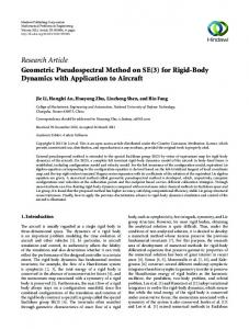
Mathematical Problems in Engineering Step 7. Since solving the NLP from the geometric pseudospectral method results in controls at only the interior points, it is necessary to obtain the endpoint controls after the NLP is solved. The method for endpoint control computation is to employ the Pontryagin minimum principle using the endpoint values of the state and costate. Remark 11. Since Steps 3∼7 are more or less the same as those of [25], the repetitious details need not be given here. 4.3. Simulation Example. In this section, we take controlling an underactuated 3D pendulum as an example to examine the performance of the previous method. The 3D pendulum (illustrated in Figure 3) is, simply, a rigid body, supported at a fixed pivot point, which has three rotational degrees of freedom; it is acted on by a uniform gravity force and,

𝑅𝑎𝑏

11 perhaps, by control and disturbance forces and moments [26]. The attitude kinematics and dynamics of the pendulum on SO(3) are given by 𝑏 ̂𝑎𝑏 𝑅̇ 𝑎𝑏 (𝑡) = 𝑅𝑎𝑏 (𝑡) ⋅ 𝜔 (𝑡) , 𝑏 𝑏 𝑏 𝑇 𝜔̇ 𝑎𝑏 (𝑡) = 𝐽−1 [𝐽𝜔𝑎𝑏 (𝑡) × 𝜔𝑎𝑏 (𝑡) + 𝑚𝑔𝜌 × 𝑅𝑎𝑏 (𝑡) 𝑒3

+ 𝐵𝑢 (𝑡)] , where the attitude configuration 𝑅𝑎𝑏 (𝑡) is a generalized coordinate of the rotation angular configuration of the bodyfixed frame {𝑂 − 𝑋󸀠 𝑌󸀠 𝑍󸀠 } relative to the inertial frame {𝑂 − 𝑋𝑌𝑍}, satisfying

cos 𝜃 cos 𝜓 − cos 𝜙 sin 𝜓 + sin 𝜙 sin 𝜃 cos 𝜓 sin 𝜙 sin 𝜓 + cos 𝜙 sin 𝜃 cos 𝜓 [ ] [ ] = [ cos 𝜃 sin 𝜓 cos 𝜙 cos 𝜓 + sin 𝜙 cos 𝜃 sin 𝜓 − sin 𝜙 cos 𝜓 + cos 𝜙 sin 𝜃 sin 𝜓] , [ ] sin 𝜙 cos 𝜃 cos 𝜙 cos 𝜃 [ − sin 𝜃 ]

where 𝜙, 𝜃, 𝜓 denote the Euler angles and the angular velocity 𝑏 vector 𝜔𝑎𝑏 (𝑡) in the body-fixed frame could be represented as 𝑇 [𝑝, 𝑞, 𝑟] , in which 𝑝, 𝑞, 𝑟 denote the angular velocity component, respectively, about 𝑋-, 𝑌-, and 𝑍-body axes. Thus, 𝑏 ̂𝑎𝑏 (𝑡) is equal to [0, −𝑟, 𝑞; 𝑟, 0, −𝑝; −𝑞, 𝑝, 0]. The conservative 𝜔 ∗ (𝑡)𝜕𝑅𝑎𝑏 (𝑡) 𝑉(𝑅𝑎𝑏 (𝑡)) could be easily obtained as 𝑚𝑔𝜌 × force 𝑅𝑎𝑏 𝑇 𝑅𝑎𝑏 (𝑡)𝑒3 , where 𝑚 is the mass of the pendulum and 𝜌 is body-fixed vector from the pivot to the center of mass of the pendulum. 𝑒3 = [0, 0, 1]𝑇 denotes the direction vector of gravity in the inertial coordinate frame. The nonconservative force 𝑇ext (𝑡) satisfies 𝐵𝑢(𝑡) with 𝐵 being the constant conjugate vector and the control vector 𝑢(𝑡) could be represented as [𝑢1 , 𝑢2 ]𝑇 , in which 𝑢1 , 𝑢2 denote the control components about 𝑋- and 𝑌-body axes, respectively. The detailed properties of the 3D pendulum are presented in Table 2. Consider the OAC problem of the 3D pendulum on SO(3), which is to control the pendulum from the initial fixed angle (𝜙0 , 𝜃0 , 𝜓0 ) and the initial fixed angular velocity (𝑝0 , 𝑞0 , 𝑟0 ) to the terminal fixed angle (𝜙𝑓 , 𝜃𝑓 , 𝜓𝑓 ) and the terminal fixed angular velocity (𝑝𝑓 , 𝑞𝑓 , 𝑟𝑓 ) with the minimum moment of the external force. The simulation parameters of the OAC problem are presented in Table 3. The proposed optimal control method (LG-GPC) is also compared with the prior works in [7, 9–11], which are also based on geometrically exact computations (Lie group variational integrator) on SO(3). There are two major categories of methods for solving the discrete first-order optimal necessary conditions derived from the optimal control problem: the nonlinear root-finding method (NRF) and the shooting method. In terms of the former, Bloch et al. [9] and Hussein et al. [10] propose a geometric structure-preserving optimal control method on SO(3), which applies a standard Newton

(63)

(64)

iterative approach to solve the discrete first-order necessary optimality conditions. However, this method does not consider the moment of the conservative force and therefore could not be compared with our method immediately. To this end, we resort to a more general discrete geometric optimal control method on Lie groups proposed in [11], which consider both the moment of conservative force and that of external nonconservative force. In this method, for the 3D pendulum, the dimension of discrete decision variables is 3(2𝑁 + 1) with the discretization number 𝑁 being 15 and the maximum iterative number being 2𝑒4 . Termination tolerances on the constraint violation, the function value, and argument are 1𝑒−6 , 1𝑒−4 , and 1𝑒−6 , respectively. In terms of the latter, Lee et al. [7] use a line search with the backtracking algorithm, referred to as “Newton-Armijo iteration (NAI),” to solve the discrete first-order necessary optimality conditions, where the time stepsize is ℎ = 0.001 s and the number of integration steps is 𝑁 = 1000. Figure 4 gives the optimal states and controls obtained from the LG-GPC method when compared with LG-PC and NRF. As seen from Figure 4, the results obtained from LGGPC and LG-PC satisfy the boundary condition of states and control, except those of NRF, because the first two could consider constraints of states and control explicitly, the latter has no choice but to introduce a dummy factor. Table 4 illustrates the optimal costs J and operation time 𝑡 of LGGPC, LG-PC, NRF, and NAI. It is concluded from the optimal costs that the methods based on LGVI are superior to LGGPC and LG-PC, since the former belong to indirect method that is higher in accuracy. However, the last two have not only larger convergence radius, but also higher convergence rate. With the numerical advantage of the geometric collocation discretization, LG-GPC has the least operation time.

2 0

0.2

0.4

0.6

0.8

1 𝜃 (rad)

2 0

0

0.2

0.4

0.6

0.8

1

2 0

2 0 −2

0

0.2

0.4

0.6

0.8

1

0

0.2

0.4

0.6

0.8

1

0

0.2

0.4

0.6

0.8

1

1

𝜓 (rad)

𝜃 (rad)

0

𝜓 (rad)

𝜙 (rad)

Mathematical Problems in Engineering

𝜙 (rad)

12

0

0.2

0.4

0.6

0.8

1

0 −1 2 0 −2

t (s)

t (s)

LG-GPC LG-PC

NRF (b) Angular configuration versus time

2 0 −2

p (rad/s)

p (rad/s)

(a) Angular configuration versus time

0.4

0.6

0.8

1

2 0 −2 0

0.2

0.4

0.6

0.8

20 0 −20

1

2 0 −2

r (rad/s)

r (rad/s)

0.2

q (rad/s)

q (rad/s)

0

20 0 −20

0

0.2

0.4

0.6

0.8

1

0

0

×10 5 0 −5 0

0.2

0.4

0.6

0.8

1

0.2

0.4

0.6

0.8

1

0.2

0.4

0.6

0.8

1

0.6

0.8

1

0.6

0.8

1

−7

t (s)

t (s) NRF

LG-GPC LG-PC

(d) Angular velocity versus time

(c) Angular velocity versus time

30 u1 (Nm)

u1 (Nm)

5

0

−5

0

0.2

0.4

0.6

0.8

0 0

0.2

0.4

0

0.2

0.4

30 u2 (Nm)

u2 (Nm)

10

−10

1

5

0

−5

20

0

0.2

0.4

0.6

0.8

1

20 10 0 −10

t (s)

t (s) NRF

LG-GPC LG-PC (e) Control versus time

(f) Control versus time

Figure 4: The optimal state and control of the pendulum obtained by LG-GPC, LG-PC, and NRF.

Mathematical Problems in Engineering

13

Acknowledgment

Table 2: Properties of a 3D rigid pendulum [7]. Physical quantity Mass

Moment of inertia

Symbol

Value

𝑚

1 kg

𝐽

0.156 0 [ [ [ 0 0.156 [ [ 0

𝜌

Vector of pivot Conjugate vector

𝐵

Weighting matrix

𝑃

This work was supported by the National Natural Science Foundation of China (61403410). 0

] ] kg⋅m2 0] ]

0 0.3] [0, 0, 0.75]𝑇 m 1 0 0 [ ] 0 1 0 [ ] 𝐼2×2

𝑇

Table 3: The simulation parameters of the OAC problem. Decision variable 𝜙 (rad) 𝜃 (rad) 𝜓 (rad) 𝑝 (rad/s) 𝑞 (rad/s) 𝑟 (rad/s) 𝑢1 (N⋅m) 𝑢2 (N⋅m)

Initial value 0 0 0 0 0 0 — —

Terminal value 𝜋 0 𝜋/2 0 0 0 — —

Boundary condition [−𝜋, 𝜋] [−𝜋, 𝜋] [−𝜋, 𝜋] [−𝜋, 𝜋] [−𝜋, 𝜋] [−𝜋, 𝜋] [−5, 5] [−5, 5]

Initial guess 0 0 0 0 0 0 0 0

Table 4: Optimized performance index and operation time. J 𝑡

LG-GPC 11.3466 4.3838

LG-PC 10.9628 4.8782

NRF 2.1044 154.7895

NAI 1.52 —

5. Conclusions This paper shows how to apply the pseudo-spectral collocation method to a constrained OAC problem for a rigid body on SO(3). First, we establish a left-invariant rigid-body attitude dynamical model in a body-fixed frame on SO(3). Then, we propose a geometric collocation method which has a comprehensive advantage in accuracy, computational efficiency, and the Lie group structural conservativeness. Preservation of key motion invariance leads to robust dynamics approximation. Finally, the proposed method is applied to a constrained OAC problem. For future work, we will further compare the method with more typical numerical methods in the Euclidean space and on the Lie group, to test the efficiency of our method. Moreover, we will extend the proposed method to a broader category of left-invariant rigid-body dynamics systems in engineering.

Conflict of Interests The authors declare that there is no conflict of interests regarding the publication of this paper.

References [1] A. V. Rao, “A survey of numerical methods for optimal control,” in Proceedings of the AAS/AIAA Astrodynamics Specialist Conference, AAS Paper 09-334, AAS/AIAA, Pittsburgh, Pa, USA, August 2009. [2] F. Lewis and V. Syrmos, Optimal Control, John Wiley & Sons, 1995. [3] L. S. Pontryagin, V. Boltyanskii, R. Gamkrelidze, and E. Mischenko, The Mathematical Theory of Optimal Processes, Interscience Publishers, New York, NY, USA, 1962. [4] H. B. Keller, Numerical Solution of Two Point Boundary Value Problems, SIAM, 1976. [5] J. Stoer and R. Bulirsch, Introduction to Numerical Analysis, vol. 12 of Texts in Applied Mathematics, Springer, New York, NY, USA, 2002. [6] F. Bullo and R. Murray, “Proportional derivative (PD) control on the Euclidean group,” in Proceedings of the European Control Conference (ECC ’95), Rome, Italy, September 1995. [7] T. Lee, M. Leok, and N. H. McClamroch, “Optimal attitude control of a rigid body using geometrically exact computations on SO(3),” Journal of Dynamical and Control Systems, vol. 14, no. 4, pp. 465–487, 2008. [8] T. Lee, Computational Geometric Mechanics and Control of Rigid Bodies, ProQuest, Ann Arbor, Mich, USA, 2008. [9] A. M. Bloch, I. I. Hussein, M. Leok, and A. K. Sanyal, “Geometric structure-preserving optimal control of a rigid body,” Journal of Dynamical and Control Systems, vol. 15, no. 3, pp. 307–330, 2009. [10] I. I. Hussein, M. Leok, A. K. Sanyal, and A. M. Bloch, “A discrete variational integrator for optimal control problems on SO(3),” in Proceedings of the 45th IEEE Conference on Decision & Control, pp. 6636–6641, IEEE, San Diego, Calif, USA, December 2006. [11] M. B. Kobilarov and J. E. Marsden, “Discrete geometric optimal control on lie groups,” IEEE Transactions on Robotics, vol. 27, no. 4, pp. 641–655, 2011. [12] R. Moulla, L. Lef`evre, and B. Maschke, “Geometric pseudospectral method for spatial integration of dynamical systems,” Mathematical and Computer Modelling of Dynamical Systems, vol. 17, no. 1, pp. 85–104, 2011. [13] K. Engø, “On the construction of geometric integrators in the RKMK class,” Tech. Rep. 158, Department of Computer Science, University of Bergen, Bergen, Norway, 1998. [14] R. M. Murray, Z. Li, and S. S. Sastry, A Mathematical Introduction to Robotic Manipulation, CRC Press, 1994. [15] D. A. Benson, A gauss pseudospectral transcription for optimal control [Ph.D. thesis], Department of Aeronautics and Astronautics, Massachusetts Institute of Technology, Cambridge, Mass, USA, 2004. [16] H. Munthe-Kaas, “Runge-kutta methods on Lie group,” BIT, vol. 35, pp. 572–587, 1995. [17] J. S. Hesthaven, S. Gottlieb, and D. Gottlieb, Spectral Methods for Time-Dependent Problems, Cambridge University Press, 2007. [18] J. T. Betts, “Survey of numerical methods for trajectory optimization,” Journal of Guidance, Control, and Dynamics, vol. 21, no. 2, pp. 193–207, 1998.

14 [19] T. Lee, N. H. McClamroch, and M. Leok, “A lie group variational integrator for the attitude dynamics of a rigid body with applications to the 3D pendulum,” in Proceedings of the IEEE Conference on Control Applications (CCA ’05), pp. 962–967, IEEE, Toronto, Canada, August 2005. [20] A. Iserles, H. Z. Munthe-Kaas, S. P. Nørsett, and A. Zanna, “Liegroup methods,” Acta Numerica, vol. 9, pp. 215–365, 2000. [21] A. Iserles and S. P. Nørsett, “On the solution of linear differential equations in Lie groups,” Philosophical Transactions of the Royal Society A, vol. 357, no. 1754, pp. 983–1020, 1999. [22] L. N. Trefethen, Spectral Methods in Matlab, SIAM, Philadelphia, Pa, USA, 2000. [23] J. R. Dormand and P. J. Prince, “A family of embedded RungeKutta formulae,” Journal of Computational and Applied Mathematics, vol. 6, no. 1, pp. 19–26, 1980. [24] E. Hairer, C. Lubich, and G. Wanner, Geometric Numerical Integration: Structure-Preserving Algorithms for Ordinary Differential Equations, vol. 31 of Springer Series in Computational Mathematics, Springer, Berlin, Germany, 2002. [25] A. V. Rao, D. A. Benson, C. L. Darby et al., “Algorithm 902: GPOPS, a MATLAB software for solving multiple-phase optimal control problems using the gauss pseudospectral method,” ACM Transactions on Mathematical Software, vol. 37, no. 2, article 22, 2010. [26] J. Shen, A. K. Sanyal, N. A. Chaturvedi, D. Bernstein, and N. H. McClamroch, “Dynamics and control of a 3D pendulum,” in Proceedings of the 43rd IEEE Conference on Decision and Control (CDC ’04), pp. 323–328, Paradise Island, Bahamas, December 2004.

Mathematical Problems in Engineering

Advances in

Operations Research Hindawi Publishing Corporation http://www.hindawi.com

Volume 2014

Advances in

Decision Sciences Hindawi Publishing Corporation http://www.hindawi.com

Volume 2014

Journal of

Applied Mathematics

Algebra

Hindawi Publishing Corporation http://www.hindawi.com

Hindawi Publishing Corporation http://www.hindawi.com

Volume 2014

Journal of

Probability and Statistics Volume 2014

The Scientific World Journal Hindawi Publishing Corporation http://www.hindawi.com

Hindawi Publishing Corporation http://www.hindawi.com

Volume 2014

International Journal of

Differential Equations Hindawi Publishing Corporation http://www.hindawi.com

Volume 2014

Volume 2014

Submit your manuscripts at http://www.hindawi.com International Journal of

Advances in

Combinatorics Hindawi Publishing Corporation http://www.hindawi.com

Mathematical Physics Hindawi Publishing Corporation http://www.hindawi.com

Volume 2014

Journal of

Complex Analysis Hindawi Publishing Corporation http://www.hindawi.com

Volume 2014

International Journal of Mathematics and Mathematical Sciences

Mathematical Problems in Engineering

Journal of

Mathematics Hindawi Publishing Corporation http://www.hindawi.com

Volume 2014

Hindawi Publishing Corporation http://www.hindawi.com

Volume 2014

Volume 2014

Hindawi Publishing Corporation http://www.hindawi.com

Volume 2014

Discrete Mathematics

Journal of

Volume 2014

Hindawi Publishing Corporation http://www.hindawi.com

Discrete Dynamics in Nature and Society

Journal of

Function Spaces Hindawi Publishing Corporation http://www.hindawi.com

Abstract and Applied Analysis

Volume 2014

Hindawi Publishing Corporation http://www.hindawi.com

Volume 2014

Hindawi Publishing Corporation http://www.hindawi.com

Volume 2014

International Journal of

Journal of

Stochastic Analysis

Optimization

Hindawi Publishing Corporation http://www.hindawi.com

Hindawi Publishing Corporation http://www.hindawi.com

Volume 2014

Volume 2014