Mar 12, 2014 - the optimization task is limited to a time horizon with an initial .... tions and CPU time. ... eled under JModelica.org using a Python script. Then.
Modified Multiple Shooting Combined with Collocation Method in JModelica.org with Symbolic Calculations Evgeny Lazutkin, Abebe Geletu, Siegbert Hopfgarten, Pu Li Simulation and Optimal Processes Group, Institute for Automation and Systems Engineering, Technische Universität Ilmenau, P.O.Box 10 05 65, 98684 Ilmenau, Germany. (evgeny.lazutkin, abebe.geletu, siegbert.hopfgarten, pu.li)@tu-ilmenau.de
Abstract This paper presents an efficient and a novel implementation of a combined multiple shooting and collocation (CMSC) algorithm for the solution of nonlinear optimal control problems. The implemented algorithm is a modification of the approach proposed in [17, 18]. The new implementation is done under the JModelica.org framework along with CasADi and Ipopt. The framework uses a symbolic pre-calculation of functions and derivatives. Besides the integration of various components of JModelica.org, Ipopt, and CasADi, the implementation facilitates simpler modeling of optimal control problems along with a choice of options for various linear algebra algorithms. The paper gives a description of the algorithm and elaborates the components of the framework. Numerical experimentations show that the new implementation is efficient in comparison with the published results of other authors. Keywords: Nonlinear Optimal Control; Symbolic Automatic Differentiation; Nonlinear Programming; Multiple Shooting; Collocation
1
Introduction
Optimization methods nowadays play pivotal roles in engineering and industrial applications. Most engineering applications are dynamic by nature. Frequently, such dynamic processes have model equations involving large-scale nonlinear differential equations. Hence, the solution of large-scale optimal control problems is difficult to achieve by solving the equations of the optimality conditions. Therefore, the modern approach follows the "first discretize, then optimize" strategy. In this way, the optimal control problem will be transformed into a nonlinear programming problem (NLP). This facilitates the implementation of efficient and state-of-the-art NLP solvers to determine highly accurate approximate optimal solutions to the DOI 10.3384/ECP14096999
continuous optimal control problem. The direct discretization of optimal control problems through the multiple shooting method was first proposed in [9]. On the other hand, the direct discretization of optimal control problems through collocation methods has been widely used for state constrained optimal control problems (e.g., [7, 10, 13]). The multiple shooting discretization results in blockstructured matrices and facilitates easy parallelization of computations. However, the accuracy of the multiple shooting method can be highly augmented if it is combined with the collocation method. Therefore, recently, discretization of optimal control problems through a CMSC method is found to have enormous potentials for the solution of complex large-scale optimal control problems [17, 18]. In order to facilitate the industrial application of complex optimization algorithms, model-based optimization of dynamic systems is recently gaining greater momentum [1, 12]. The aim of this work is to implement the CMSC algorithm in the JModelica.org framework. We first divide the time horizon [t0 ,t f ] into subintervals (finite elements). Subsequently, we use multiple shooting and collocation methods to discretize the optimal control problem and to transform it into an NLP. In our implementation, we use precalculated derivatives, i.e., Jacobian matrix in symbolic form by means of CasADi [3, 4]. The nonlinear optimization problem is solved by using Ipopt (Interior point optimization solver, [19]). The total optimization tool-chain is provided in the JModelica.org framework [2]. The rest of the paper is organized as follows. Section 2 provides a general form of the considered optimal control problem. Section 3 presents the combined multiple shooting and collocation algorithm. Section 4 describes the implementation of the algorithm under the JModelica.org framework coupled with CasADi and Ipopt and section 5 presents case studies. The
Proceedings of the 10th International ModelicaConference March 10-12, 2014, Lund, Sweden
999
Modified Multiple Shooting Combined with Collocation Method in JModelica.org with Symbolic Calculations
comparative analysis in section 6 shows the high efficiency and viability of our implementation as compared to other implementations. The paper concludes in section 7 with a summary and future research work.
2
Problem definition
0, . . . , N − 1. Then, on each shooting interval [ti ,ti+1 ], collocation nodes ti = ti0 < ti1 < . . . ,tiNc = ti+1 are defined, so that each state variable xk (t) is approximated by the polynomial xˆk (t) =
Nc
∑ xi j
(k)
li j (t),
(7)
j=0
We consider the following general form of a nonlinear where li j (t) are the Lagrange polynomials optimal control problem (NOCP): � � � Z tf Nc � t − tis min J = E (x(t f )) + (1) L(x(t), u(t),t)dt li j (t) = ∏ , j = 1, . . . , Nc , i = 1, . . . , N, u(t) t0 ti j − tis s=0 subject to: x(t) ˙ = f (x(t), u(t),t), x(t0 ) = x0 , (2) s 6= j g(x(t), u(t),t) = 0, (3) (8) xmin ≤ x(t) ≤ xmax , (4) and the variables x(k) , j = 1, . . . , Nc , represent the state ij umin ≤ u(t) ≤ umax , (5) values corresponding to the state variable xk (t), k = t0 ≤ t ≤ t f , (6) 1, . . . , n, at the collocation points on [ti ,ti+1 ] with the (k) property that xk (ti j ) = xˆk (ti j ) = xi j . Hence, the comwhere x(t)> = (x1 (t), . . . , xn (t)) and u(t)> = bined multiple shooting and collocation scheme trans(u1 (t), . . . , um (t)) are the state and control vec- forms the NOCP into an NLP with the additional contors, respectively. The functions f , h, and g are straints conveniently defined in appropriate function spaces. The dynamics of the process is described by (2) hki+1 = xˆk (t(i+1)0 ), i = 0, . . . , N − 1; k = 1, . . . , n (9) and we have algebraic equality constraints (3). In practical engineering or industrial application, state to be imposed along with the discretized constraints and control variables are usually bounded. Hence, (4) (2)-(5). The equations (9) guarantees the continuity of imposes lower and upper bounds on the states, while the state trajectories at the end point of each shooting �> (5) defines bounds on the controls. The optimization interval. In the following hxi+1 = h1i+1 , . . . , hni+1 � variables (typically the controls) and state variables and xˆi+1 (hx , vi ,ti+1 ) = xˆ1 (t(i+1)0 ), . . . , xˆn (t(i+1)0 ) > i must satisfy the model equations, the state and control are used for the sake of brevity. The expression constraints and the boundary conditions. Furthermore, xˆi+1 (hx , vi ,ti+1 ) indicates that the state variables are i the optimization task is limited to a time horizon with dependent on the initial state hx , the controls vi and i an initial time t0 and a fixed final time t f . In this paper, the end time point t(i+1)0 = ti+1 on the interval [ti ,ti+1 ]. time-optimal control problems will not be considered. The resulting nonlinear optimization problem can be The optimal control problem (1) - (6) is an infinite- written as ( ) dimensional problem. Since real-world applications N−1 x x min E (hN ) + ∑ L(hi , xi , vi ) (10) have very complicated structure including nonlinearity hx0 ,...,hxN ,v0 ,...,vN−1 i=0 and high dimensionality, indirect methods, like methx x subject to: hi+1 − xˆi+1 (hi , vi ,ti+1 ) = 0, ods based on the Pontryagin’s principle, are not suitable. Therefore, here the NOCP will be directly disi = 0, . . . , N − 1, (11) x cretized by using a combined multiple shooting and G(hi , xi , vi ) = 0, i = 0, . . . , N − 1, (12) collocation (CMSC) method and thereby it will be hx0 − x0 = 0, (13) transformed to a finite-dimensional optimization probx xmin ≤ hi ≤ xmax , (14) lem. umin ≤ vi ≤ umax , (15)
3
An improved multiple shooting with collocation framework
In problem (10) - (15) on the i-th shooting subinterval, hxi represents parameterized initial conditions for the vector of state variables, xˆi is the state on the collocaFor the multiple shooting and collocation discretiza- tion point at the end of interval i, the vector xi consists tion scheme, first the time interval [t0 ,t f ] is di- of all coefficients of the collocation polynomials corvided into appropriate shooting intervals [ti ,ti+1 ], i = responding to the states on the i-th interval and vi are 1000
Proceedings of the 10th International ModelicaConference March 10-12, 2014, Lund, Sweden
DOI 10.3384/ECP14096999
Session 6C: Optimization Applications and Methods
parameterized control variables. The discretization of the states uses the Radau collocation method. Using the function G, equation (12) represents the discretized form of the equations (2, 3). The control variables are usually parameterized as piecewise constant functions. E.g., in each subinterval [ti ,ti+1 ], i = 0, . . . , N − 1, the control variables are assumed to take constant values and the state trajectories will be approximated by the collocation method. The unique feature of CMSC lies in the fact that it utilizes the advantages of both multiple shooting and collocation methods. Detailed discussions on multiple shooting and collocation methods are found in [8, 9, 16]. In the objective (10) the variable x does not appear exclusively as an optimization variable. Hence, after appropriate aggregation of variables, at each step of the optimization algorithm, we can solve for x in terms of (h, v), so that we have x(h, v). In this way the equality constraints (12) can be eliminated by reducing the number of optimization variables. However, in this work, constraints on the coefficients of the collocation polynomials are not considered inside the collocation intervals, but only at the end-points of the intervals. Therefore, the problem (10) - (15) can be equivalently written as min F(h, x(h, v), v) h,v
subject to : H(h, v) = 0 xmin ≤ h ≤ xmax
umin ≤ v ≤ umax ,
Algorithm 1 : A general CMSC 1: Input: Time horizon, number of subintervals, number of state and control variables, lower and upper bounds for the control and state variables, model equations, objective function, initial guesses, optimizer options. 2: Initialization of the NOCP 3: Define continuity and path constraints 4: Initialize the n-point collocation for each subinterval 5: Compute states at collocation points and sensitivities 6: Compute objective function and gradient 7: Compute constraint function values and Jacobian 8: Solve the equations of the Karush-Kuhn-Tucker (KKT) optimality conditions 9: if KKT condition not satisfied then 10: GOTO 3 11: else 12: STOP. 13: end if 14: Output: optimal state and control trajectories, optimal objective function value, number of itera(16) tions and CPU time. (17) (18) (19)
where H in equation (17) provides a compact representation of the equations (11) - (13). Consequently, to solve the nonlinear optimization problem (16) - (19) we use the state-of-the-art optimization solver Ipopt [19]. At each iteration of Ipopt, the nonlinear model equations are solved by using a local Newton algorithm along with a linear algebra solver for the determination of the Newton-steps to determine state variables for given values of h and v. Future investigations will consider the implementation of a globalized Newton method with appropriate linear algebra solvers. All function values and gradients, required in the optimization framework, are pre-calculated and made available in symbolic form. Symbolic derivatives are calculated by using CasADi and stored in matrices or vectors to facilitate faster accessability. For this, it is needed to compute the sensitivities ∂∂Fv , ∂∂Fh , ∂∂Hv , and ∂H ∂ h in symbolic representations. Further details are found in [17, 18]. The computational framework is summarized DOI 10.3384/ECP14096999
graphically in Fig. 1 and Algorithm 1 provides a description in general terms. More detailed discussions on the CMSC method are found in [17, 18].
Figure 1: : Combined multiple shooting and collocation (CMSC) framework Algorithm 1 is general for CMSC from the work of [17, 18]. This work implements a modified and improved version of Algorithm 1. Hence, Algorithm 2 provides a modified CMSC.
Proceedings of the 10th International ModelicaConference March 10-12, 2014, Lund, Sweden
1001
Modified Multiple Shooting Combined with Collocation Method in JModelica.org with Symbolic Calculations
Algorithm 2 : A modified CMSC 1: Input: Time horizon, number of subintervals, number of state and control variables, lower and upper bounds for the control and state variables, model equations, objective function, initial guesses, optimizer options, number of collocation points in subintervals, user-defined options, e.g., choice of a linear algebra algorithms, etc. 2: Calculate in symbolic form the Jacobian of the system and all directional derivatives. 3: Corresponding to the number of subintervals, states/controls, and collocation points, construct derivative matrices 4: Initialize and construct symbolic representations of the objective function and corresponding gradient. 5: Initialize and construct symbolic representation of the constraint functions and corresponding Jacobian. 6: Give an initial guess for the optimization variables 7: Set options for Ipopt to provide Hessian approximation, tolerance of the solution, and other user specified options. 8: Call the Ipopt solver 9: Call plotting routine and save the results.
invokes Ipopt to solve the NLP by using the precalculations. All problem definitions and our custom implementations are done using the Python programming language.
Figure 2: : Software framework In the next subsections, we give a brief review on the software components.
4.1
JModelica.org
JModelica.org [2] is a Modelica-based open source software platform for modeling and solving optimal control problems and implementation of userdeveloped algorithms. JModelica.org was first developed at the Department of Automatic Control, Lund University. Currently, it enjoys active support from the The improvements provided in Algorithm 2 are: industry (Modelon AB) as well as academic and re• the symbolic pre-calculation to obtain represen- search institutions. Since JModelica.org is extensible tations for the values of the objective function, through user-designed algorithms, we have decided to constraints, and corresponding sensitivities (Ja- implement our algorithm under this framework. Among the salient features of JModelica.org are: cobians and derivatives), • facilitate the use of several linear algebra algorithms to give the user a choice of options and improve the efficiency of computations, • implementation on JModelica.org platform for a wider public accessibility.
Section 4 discusses the software implementation of Algorithm 2.
4
• easy and smoother integrability of custom numerical libraries, • support for object-oriented modeling based on Modelica, • wider public access owing to simpler user interfaces.
Framework and software compo4.2 CasADi nents
In the framework shown in Fig. 2, the NOCP is modeled under JModelica.org using a Python script. Then the problem is discretized using our CMSC with the help of CasADi to obtain an NLP. Subsequently, CasADi is again invoked to generate symbolic expressions for the derivatives. Finally, JModelica.org 1002
• support for mixed-language programming mode,
CasADi is an open source software library for symbolic automatic differentiation of functions [5]. CasADi uses computer algebra techniques to implement the forward and adjoint automatic differentiation techniques and facilitate the pre-computation of gradients and Jacobian of objective functions and constraints, respectively.
Proceedings of the 10th International ModelicaConference March 10-12, 2014, Lund, Sweden
DOI 10.3384/ECP14096999
Session 6C: Optimization Applications and Methods
One of the major features of CasADi is its high integrability to widely available open source numerical libraries and optimization solvers. CasADi is written using C++ programming language. However, it can be interfaced to numerical solvers based on various programming language implementations, e.g., C, C++, Python, FORTRAN, etc. The recent integration of CasADi to the JModelica.org platform [4] is one proof for its high integrability and applicability for the solution of complex optimal control problems. Therefore, in our implementation, we have exploited the potential of CasADi for symbolic pre-computation of derivatives in order to improve the efficiency of computations.
4.3
5.1
A nonlinear batch-reactor
The system has two state variables x1 (t) and x2 (t) (corresponding to concentrations of two species) and one control variable u(t) (reaction temperature). The objective of this benchmark problem is to achieve a maximum product output of x2 (t f ). The NOCP is formulated as follows: max x2 (t f )
(23)
u(t)
subject to :
� � u2 (t) x˙1 (t) = − u(t) + · x1 (t), (24) 2 x˙2 (t) = u(t) · x1 (t), (25)
x1 (t0 ) = 1,
Ipopt
(26)
x2 (t0 ) = 0, (27) � � Ipopt is a software implementation of an interior point x1 (t) 0≤ ≤ 1, (28) algorithm coupled with a filter line-search algorithm x2 (t) [19]. Ipopt is a state-of-the-art solver for large-scale 0 ≤ u(t) ≤ 5, (29) NLP problems. Consequently, it facilitates the effi0 ≤ t ≤ 1. (30) cient solution of large-scale optimal control problems using the "first discretize, then optimize" approach. The objective function in equation (23) describes the In general, Ipopt can be used to solve NLP problems amount of output of the second species at the fiof the form nal time. This example has been also studied in [6, 14, 17, 18]. minn f (x) (20) x∈R
x1
subject to :
1.0 0.8 gmin ≤ g(x) ≤ gmax , (21) 0.6 xmin ≤ x ≤ xmax , (22) 0.4 0.2 0.00.0 n where f (x) : R → R is the objective function, and Rn
Rm
g(x) : → is the constraint function. The vectors xmin and xmax are the bounds on the variables x, and the vectors gmin and gmax denote the lower and upper bounds on the constrained function g(x). Furthermore, equality constraints can also be stated in the above formulation by setting the corresponding components of gmin and gmax to the same value. The functions f (x) and g(x) can be nonlinear and non-convex. Theoretically, f (x) and g(x) are required to be twice continuously differentiable. However, Ipopt is capable of working with first order information, so that Hessian matrices can be approximated numerically.
5
Case studies
0.2
0.4
0.6 0.5 0.4 0.3 0.2 0.1 0.00.0
0.2
0.4
5 4 3 2 1 00.0
0.2
0.4
x2
u
Time
0.6
0.8
1.0
0.6
0.8
1.0
0.6
0.8
1.0
Figure 3: : Optimal solution of the NOCP (23) - (30)
The results shown in the Fig. 3 is obtained by using To investigate the performance of the modified Algorithm 2 with 160 subintervals. In the next secmethod, the following two case studies are considered. tion we will present a comparative analysis of results DOI 10.3384/ECP14096999
Proceedings of the 10th International ModelicaConference March 10-12, 2014, Lund, Sweden
1003
Modified Multiple Shooting Combined with Collocation Method in JModelica.org with Symbolic Calculations
obtained from our Algorithm 2 and similar solution collocation on each subinterval. This leads to an NLP with 507 variables and 357 constraints. The results of methods of other authors. our implementation are depicted in Figs. 4 - 6.
5.2
A satellite control problem
A nonlinear optimal control problem of a rigid satellite initially undergoing a tumbling motion is considered. The problem data are given as follows [17]: • I1 = 106 , I2 = 833333, I3 = 916677 represent principal moments of inertia, respectively • T1s = 550, T2s = 50, T3s = 550 are time constants • Initial states: x1 (0) = 0, x2 (0) = 0, x3 (0) = 0, x4 (0) = 1, x5 (0) = 0.01, x6 (0) = 0.005, x7 (0) = 0.001 • Time horizon: [t0 ,t f ] = [0, 100] • Fixed terminal state: xt>f = (0.70106, 0.0923, 0.56098, 0.43047, 0, 0, 0)
x1
0.5 0.4
0.20
0.3
0.15
0.2
0.10
0.1
0.05
0.00
20
40
0.10
x3
60
80
100 0.000
20
40
80
1.00 0.98 0.96 0.94 0.92 0.90 0.88 0.86 0.84 100 0.820
20
40
0.08 0.06 0.04 0.02 0.000
20
40
Time
x2
0.25
60
x4
Time
60
80
100
60
80
100
Figure 4: : Optimal states x1 - x4
The aim of the optimal control is to determine the x5 x7 0.0030 torques that bring the satellite to rest in the specified 0.0105 time t f = 100, while minimizing the performance in- 0.0104 0.0103 dex. The NOCP is defined as follows [17]: 0.0025 0.0102 � � Z 1 tf 2 2 min kx(t f ) − x f k + kuk dt (31) 0.0101 2 t0 u(t) 0.01000 20 40 60 80 100 0.0020 1 x6 subject to: x˙1 = (x5 x4 − x6 x3 + x7 x2 ) (32) 0.00505 2 0.00500 1 x˙2 = (x5 x3 + x6 x4 − x7 x1 ) (33) 0.00495 0.0015 2 0.00490 1 x˙3 = (−x5 x2 + x6 x1 − x7 x4 ) (34) 0.00485 2 0.00480 1 0.004750 20 40 60 80 100 0.00100 20 40 60 80 100 x˙4 = − (x5 x1 + x6 x2 + x7 x3 ) (35) Time Time 2 (I2 − I3 ) x6 x7 + T1s u1 x˙5 = (36) Figure 5: : Optimal states x5 - x7 I1 (I3 − I1 ) x7 x5 + T2s u2 x˙6 = (37) It takes 291 milliseconds of CPU time for the comI2 putation and the obtained optimal value of the objec(I1 − I2 ) x5 x6 + T3s u3 x˙7 = . (38) tive function is 0.463968. In contrast, the optimal I3 value of the objective function in [17] is 0.468287 obHere x> (t) = (x1 (t), . . . , x7 (t)) is the state vector and tained in 531 milliseconds of CPU time. u> (t) = (u1 (t), u2 (t), u3 (t)) is the control vector of the torques acting for the respective body-principle axes. 6 Comparative analysis The model equations (32) - (35) are the kinematic equations associated to the orientation and (36) - (38) In this section we use the problem (23) - (30) for the are the dynamic equations associated to the motion of purpose of comparison. Tables 1 - 4 present results the satellite. The state variables x1 (t) - x4 (t) are the obtained from similar, but different optimization methEuler parameters and x5 (t) - x7 (t) are the angular rates. ods. Note, that these results have been obtained using To solve this problem using Algorithm 2, we divide different computational platforms. Nevertheless, some the time horizon into 50 subintervals and use a 3-point ideas can be gained by observing the results obtained. 1004
Proceedings of the 10th International ModelicaConference March 10-12, 2014, Lund, Sweden
DOI 10.3384/ECP14096999
Session 6C: Optimization Applications and Methods
0.025 0.020 0.015 0.010 0.005 0.0000 0.00030 0.00025 0.00020 0.00015 0.00010 0.00005 0.000000 0.030 0.025 0.020 0.015 0.010 0.005 0.0000
u1
Table 3: Comparative results from discretization (5 subintervals) Objective function
20
40
20
40
u2
u3
60
80
60
80
100
Modified CMSC CMSC by [17] Collocation algorithm by [15] Multiple shooting by [14]
100
Number of constraints
0.56817 0.56817 0.57302
Number of optimization variables 17 18 101
0.56838
18
10
12 12 86
Table 4: Comparative results from discretization (160 subintervals) 20
40
Time
60
80
Objective function
100 Modified CMSC CMSC by [17] Collocation algorithm by [15] Multiple shooting by [14]
Figure 6: : Optimal controls u1 (t), u2 (t), u3 (t)
Number of constraints
0.57354 0.57354 0.57354
Number of optimization variables 482 483 3046
0.57354
483
320
322 322 2566
However, our modified CMSC algorithm is comparable to the collocation algorithm suggested in [15], As shown in Table 4, our Algorithm 2 shows a since the implementation in [15] and of our modified higher performance in terms of CPU time as compared CMSC are both done on the same type of computer to all presented algorithms, still obtaining the the same with 3.2 GHz CPU frequency. objective function value as reported by other authors. Table 1: CPU time (in milliseconds) Number of subintervals 5 10 20 40 80 160 320
Modified CMSC 4 6 8 12 24 40 81
CMSC [17] 188 290 350 480 547 735 NaN
Collocation [15] 4 8 12 20 48 102 268
Multiple Shooting [14] Unc., Sp. Con., Co. 4 3 6 5 9 9 12 17 24 57 58 341 159 2717
In Tables 1 and 2 • Unc.: uncondensed SQP, • Con.: condensed SQP, • Sp.: Block structured QP solver using MA57, • Co.: Matrix condensing and dense QP solver qpOASES [11].
Number of subintervals 5 10 20 40 80 160 320
Table 2: Number of iterations
Modified CMSC 14 16 19 22 27 18 14
CMSC [17] 16 21 21 25 23 23 27
Collocation [15] 17 24 21 20 23 23 27
Multiple Shooting [14] Unc., Sp. Con., Co. 7 7 9 9 9 9 10 10 10 11 12 12 12 14
As shown in Tables 1 and 2, the modified CMSC method performs more efficient, both in terms of CPU time and number of iterations, as compared to pure simultaneous (collocation) method. This facilitates the future use of Algorithm 2 for the model predictive control scheme on longer prediction horizons. Considering Table 3, for the discretization using 5 subintervals, the collocation scheme of [15] provides lower function values as compared to Algorithm 2, but the CPU time of the modified CMSC method is better than the one reported in [17]. DOI 10.3384/ECP14096999
7
Conclusion and future work
This paper presents the first prototype of a modified combined multiple shooting and collocation method. The major difference from the original version of the CMSC approach in [17, 18] consists in using precalculated derivatives and their symbolic representation. That is, in every iteration of the optimization algorithm, sensitivities are automatically available without further calculations. The optimizer is provided with symbolic derivatives which are to be evaluated at the given iterate. This leads to accurate results with speedup of the overall computation time. This preliminary investigation shows that the implemented algorithm has a competitive performance compared to other similar investigations. There is also a potential for parallel implementation of the proposed algorithm, whereby constraints to be considered on the coefficients of the collocation polynomials inside the shooting intervals. Furthermore, the modified CMSC method will be implemented to work directly with Modelica models along with a choice of local and global nonlinear equation solvers. Hence, the proposed framework will be refined to make it highly transparent, so that end-users can solve various types of applied optimal control problems. In addition, the algorithm will be extended to handle nonlinear model predictive control (NMPC) problems.
Proceedings of the 10th International ModelicaConference March 10-12, 2014, Lund, Sweden
1005
Modified Multiple Shooting Combined with Collocation Method in JModelica.org with Symbolic Calculations
8
Acknowledgements
[9] Bock, H. G., Plitt, K. J. A Multiple Shooting Algorithm for Direct Solution of Optimal Control Problems, Prepr. 9th IFAC World Congress, Budapest, 1984, pp. 242-247.
This work has been supported by Model Driven Physical Systems Operation project (MODRIO) by ITEA2, No. 11004, and by the German BMBF (BMBF [10] Cuthrell, J. E., Biegler, L. T.: Simultaneous optiFörderkennzeichen: 01IS12022H). s mization and solution methods for batch reactor control profiles. Comput. Chem. Eng. 13(1989), pp. 49-62. References [11] [1] Åkesson, J.: Optimica—An Extension of Modelica Supporting Dynamic Optimization. 6th International Modelica Conference, March 3 - 4, 2008, Bielefeld, Germany, pp. 57-66. [12]
Ferreau, H. J.: Model predictive control algorithms for applications with millisecond timescales. PhD Thesis, KU Leuven, 2011. Franke, R.: Formulation of dynamic optimization problems using Modelica and their efficient solution. 2nd International Modelica Conference, March 18 - 19, DLR, Oberpfaffenhofen, Germany, pp. 315 - 323.
[2] Åkesson, J., Årzén, K.-E., Gåfvert, M., Bergdahl, T., Tummescheit, H.: Modeling and optimization with Optimica and JModelica.orgLanguages and tools for solving large-scale dynamic optimization problems. Computers and [13] Hong, W., Wang, S., Li, P., Wozny, G., Biegler, Chemical Engineering, 34(2010)11, pp. 1737L. T.: A quasi-sequential approach to large-scale 1749. dynamic optimization problems. AIChE Journal, 52(2006)1, pp. 255-268. [3] Andersson, J., et. al.: Dynamic optimization with CasADi. In Proceedings of the 51st IEEE Con- [14] Kirches, C., Wirsching, L., Bock, H. G., Schlöder, J. P.: Efficient Direct Multiple Shootference on Decision and Control, Maui (USA), ing for Nonlinear Model Predictive Control on 2012. Long Horizons. J. Process Control, 22(2012), [4] J. Andersson, J., Casella, F., Diehl, M.: Integrapp. 540-550. tion of CasADi and JModelica.org. 8th Interna[15] Magnusson, F.: Collocation Methods in JModeltional Modelica Conference, Dresden, 2011. ica.org. Master Thesis, Lund University, FebruDOI:10.3384/ecp1106321 ary 2012. [5] Andersson, J., Åkesson, J., Diehl, M.: CasADi: A Symbolic Package for Automatic Differentia- [16] Russel, R. D., Shampine, L. F.: A Collocation Method for Boundary Value Problems, Numerition and Optimal Control. Lecture Notes in Comcal Mathematic, 19(1971), pp. 1-28, Springer. putational Science and Engineering, Vol. 87, Springer, 2012, pp. 297-307. [17] Tamimi, J.: Development of the Efficient Algorithms for Model Predictive Control of Fast Sys[6] Bachmann, B., Ochel, L., Ruge, V., Gebremedtems. PhD Thesis, Technische Universität Ilmehin, M., Fritzson, P., Nezhadali, V., Eriksson, nau, VDI Verlag, 2011. L., Sivertsson, M.: Parallel Multiple-Shooting and Collocation Optimization with OpenModel[18] Tamimi, J., Li, P.: A Combined approach to nonica. Proceedings of the 9th International Modellinear model predictive control of fast systems. ica Conference, Munich, pp. 659-668, 2012. J. Process Control, 20(2010)9, pp. 1092-1102. [7] Bartl, M., Li, P., Biegler, L. T.: Improvement [19] Wächter, A., Biegler, L.T.: On the Implemenof state profile accuracy in nonlinear dynamic tation of a Primal-Dual Interior Point Filter optimization with the quasi-sequential approach. Line Search Algorithm for Large-Scale NonlinAIChE Journal, 57(2011)8, pp. 2185-2197. ear Programming, Mathematical Programming, Ser. A, 106(2006)1, pp. 25-57. [8] Biegler, L. T. Nonlinear Programming: Concepts, Algorithms, and Applications to Chemical Processes. SIAM, 2010. 1006
Proceedings of the 10th International ModelicaConference March 10-12, 2014, Lund, Sweden
DOI 10.3384/ECP14096999