GEOMETRY-BASED STATISTICAL MODEL FOR RADIO ...

Progress In Electromagnetics Research B, Vol. 17, 187–212, 2009

GEOMETRY-BASED STATISTICAL MODEL FOR RADIO PROPAGATION IN RECTANGULAR OFFICE BUILDINGS Y. Chen School of Engineering University of Greenwich Chatham Maritime, Kent, ME4 4TB, UK Z. Zhang School of Computer, Electronic and Information Guangxi University Nanning 530004, China L. Hu College of Communication and Information Engineering Nanjing University of Posts and Telecommunications Nanjing 210003, China P. Rapajic School of Engineering University of Greenwich Chatham Maritime, Kent, ME4 4TB, UK Abstract—We present a new approach to the modeling of angle and time of arrival statistics for radio propagation in typical office buildings, in which the majority of interior scattering objects are either parallel or perpendicular to the exterior walls. We first describe the reradiating elements in office buildings as randomly distributed arrays of thin strips. The amount of clutter and the amount of transmission/reflection loss are then accounted for through several key parameters of the site-specific features of indoor environment, such as the layout and materials of the building under consideration. Subsequently, the important channel parameters including power azimuthal spectrum (PAS) and power delay spectrum (PDS) are Corresponding author: Y. Chen ([email protected]).

188

Chen et al.

derived. An appealing observation is that when the path angles from multiple channel trials are measured and collectively analyzed, deterministic angle clustering becomes evident. This phenomenon agrees well with the existing ray-tracing (RT) results reported by Jo et al. in buildings of this type and cannot be explained by other geometric channel models (GCMs). Furthermore, the proposed model predicts an asymmetric cluster PAS for a single-channel-trial scenario, which yields an excellent fit to the experimental data presented by Poon and Ho. Finally, we have also investigated the behaviors of the superimposed PAS and PDS under various channel conditions.

1. INTRODUCTION In recent years indoor wireless communication has become progressively more popular in the context of both voice and data communication. Various short-range radio solutions such as orthogonal frequency division multiplexing (OFDM) and ultra-wideband (UWB) techniques have been proposed for high data rate transmission in wireless personal area networks (WPANs) and baseband multiple access schemes. One imperative challenge in this area is thus the theoretical and experimental investigation of radio channels as well as the establishment of efficient models [1, 2]. There is a vast amount of literature on propagation models for indoor cluttered environments. One methodology is to characterize a “sufficiently general” channel by the fewest number of parameters, which is useful when the system designer is interested in the average behavior of the statistical ensemble of channels. This school of thought includes the stochastic ray propagation approaches [3–5], the integralgeometry-based models [6], the transport-theory-based methods [7, 8], the geometric channel models (GCMs) [2, 9–13], etc. The other method is to derive the channel properties for each particular site, which is desired when an accurate assessment of the particular site is required. Under the rubric of “sufficiently site-specific” modeling, a main approach is the ray-tracing (RT) technique (see e.g., [14– 18, 33, 34]). It assumes that the locations and reflection properties of all the important objects inhibiting propagation are accurately known. Then all the possible paths connecting the transmitter (Tx) and the receiver (Rx) are found through the specified complicated environment. Fast RT techniques have been intensively pursued in recent years to expedite the computation time [16, 17]. This paper focuses on a “sufficiently general” channel model for statistically predicting the indoor radio propagation in typical office

Progress In Electromagnetics Research B, Vol. 17, 2009

189

buildings, where the majority of the exterior and interior walls are either perpendicular or parallel to each other (a building type referred to as “normal” in [18] and also the most common layout for indoor office environments). The conventional GCMs assume that the reflectors are discrete point scatterers [2, 9–13]. Equivalently, the orientations of the reflecting surfaces are direction-nonselective, which may not hold for a normal building. As a result, these models may lead to a systematic prediction error of the channel properties for this type of buildings. For example, the measured power azimuthal spectrum (PAS) in an indoor environment exhibits an asymmetric shape in angle [19], which is in contrast to the symmetric PAS patterns suggested by other GCMs. The asymmetry in angle-of-arrival (AOA) could also be observed in a more recent indoor UWB channel measurement [20]. Moreover, RT results have shown that clustering in AOA is apparent when the paths of multiple channel trials (i.e., with a large number of random Tx and Rx positions) are superimposed [18]. This is contrary to the results predicted using other GCMs, for which a non-clustered profile is always expected. These discrepancies warrant further investigations of GCMs, which should comply with the less random directions of reflecting planes in a normal building. The main contribution of this paper is thus to introduce a new model for more appropriate characterization of radio propagation within a rectangular building. The scattering elements are modeled as randomly distributed arrays of thin strips. These strips have two primary orientations: Parallel or perpendicular to the exterior wall of the building. The Gaussian probability density function (pdf) is employed to model the actual angular variation in the proximity of these two main orientations. This direction-selective arrangement, on one hand, alleviates the problem of the unrealistic premise of fully random reflector orientations. On the other hand, it preserves a certain degree of surface irregularity that is inherent in any natural propagation environments. The amount of clutter and the amount of transmission/reflection loss are then calculated through several key parameters of the site-specific features of indoor environment, which are: 1) The complex permittivity of the building materials; 2) the average length of the strips; 3) the orientation randomness of the reflecting surfaces; 4) the number of the strips per m2 ; 5) the distance of the direct path between Tx and Rx; and 6) the angle of the direct path referenced to the building wall. Subsequently, we derive the important channel parameters including PAS and power delay spectrum (PDS), where both the single- and multiple-reflection scenarios are accounted for. However, it is generally sufficient to consider only the former case because of the equivalence of multiple and single scattering processes

190

Chen et al.

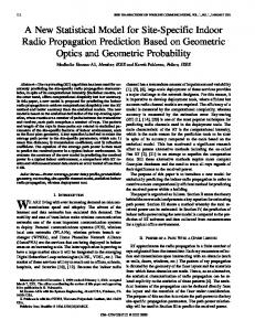
as discussed in [12]. The theoretical single-channel-trial PAS and multiple-channel-trial PAS correctly replicate the asymmetric AOA profile observed in [19] and the angle clustering reported in [18], respectively. As discussed in [21] and demonstrated through the RT data in [18], typical WPANs involve vertically polarized antennas with omnidirectional azimuthal radiation patterns and nulls at high elevation. Also, the reflection coefficients are very small when the incident radio wave reflects on the floor or the ceiling [18], thereby leading to predominantly azimuthal signal propagation. Therefore, the current work considers only two-dimensional (2-D) propagation in line with other existing indoor channel models [8, 9, 16, 18, 21, 22]). The remainder of the paper is organized as follows. Section 2 outlines the model preliminaries and derives the PAS and PDS. Starting with a single-reflection, multiple-transmission channel, the analysis is then extended to a more general multiple-reflection scenario. Subsequently, the numerical results of the field properties in indoor environments are presented in Section 3 and compared to the measured data in [19] and the RT solutions in [18]. Finally, we conclude in Section 4. 2. MODEL PRELIMINARIES AND DERIVATIONS OF CHANNEL PARAMETERS 2.1. Model Preliminaries In indoor radio channels, the signals arriving at the Rx consist of a number of multipath components originated from the Tx. Each ray is the result of the interaction of the transmitted waves with the obstacles such as walls, partitions, doors, etc.. Each time there is an obstacle-intersection the ray loses a certain amount of power while the propagation loss in between intersections will maintain the free-space rate. In this paper, we assume that transmission and reflection are two main propagation modes since other mechanisms such as diffraction and diffuse scattering are not significant in indoor environments as mentioned in [16] and [23]. This simplification has also been used in both deterministic and stochastic models in [4, 16, 18, 21] for instance. It is however possible to incorporate other propagation modes in the current model by applying a phenomenological approach following the methodology in [12]. Consider a rectangular service area filled with randomly distributed thin strips, which is relevant to a typical office building as illustrated in Fig. 1. Each strip, representing textured walls, cubicle partitions, interior doors or windows, is described by its reflection

Progress In Electromagnetics Research B, Vol. 17, 2009

Figure 1. Geometry of the proposed model. referenced to the horizontal exterior wall.

191

All the angles are

and transmission coefficients. To a first approximation, the strips are supposed to be either perpendicular or parallel to each other. It is further assumed that the external building dimension is much larger than the Tx-Rx ranges such that the boundary condition has negligible effect on the spatio-temporal channel characteristics. Let us first introduce a set of model parameters related to the propagation environment, which play a key role in the model analyzed (see also Fig. 1): • ε: The complex permittivity of building materials; ε = εr − j ωεσ 0 where εr is the relative dielectric constant, σ is the conductivity, and ε0 is the free space dielectric constant; • L: Average length of the scattering strips; • ζ: The density of the strips (in m−2 ); • D: The distance of separation between Tx and Rx; • ψ0 : The angle of the direct path between Tx and Rx referenced to an exterior wall, which is chosen to be the horizontal wall in the following discussions.

192

Chen et al.

Without loss of generality, we assume that the Tx is located at the origin of the polar coordinate. The location of each strip S is defined by the coordinates of the strip center (r, ψ), where r is the distance between Tx and S and ψ is the angle-of-departure (AOD) at the Tx relative to the horizontal exterior wall. Different from the point-scatterer representation in the existing GCMs [9–13] where the radio-wave source direction and the viewing direction are forced to converge at the scatterer, the reflection point is not uniquely defined for finite width strips. In general, the strip length is much smaller than the propagation distance from the Tx (or Rx) to S (i.e., plane wave assumption), the source and viewing directions will thus be approximately computed with reference to the strip center (r, ψ). For a lossy strip that obstructs the ray-path from Tx to S, the reflection coefficient can be calculated through the following expression by assuming a vertical polarization mode. ¯ ¯  ¯ sin ψ−√ε−cos2 ψ ¯  ¯, ¯ √  Rk,Tx→S = ¯   sin ψ+ ε−cos2 ψ ¯   when the strip to¯ the exterior wall ¯ is parallel (1) ¯ cos ψ−√ε−sin2 ψ ¯  ¯  ¯ √ R⊥,Tx→S = ¯ ,   cos ψ+ ε−sin2 ψ ¯   when the strip is perpendicular to the exterior wall The subscripts “k” and “⊥” in (1) indicate the orientations of the strips. If we seek average information about the behavior of the wave in a random medium and suppose that both the two directions are equally probable, the mean transmission loss `T,T x→S can be obtained as " r # ³ ´³ ´ m `T,T x→S = χ

2 1 − Rk,T x→S

2 1 − R⊥,T x→S

(2)

where χ is a coefficient that accounts for the penetration loss. m describes the total number of successive blocks for the ray-path from Tx to S. Apparently, an object intersection will occur when the center of a horizontal strip falls in the shaded Area I or the center of a vertical strip falls in the shaded Area II as illustrated in Fig. 1. Thus, m can be approximated as 1 m ≈ ζ (rL sin ψ + rL cos ψ) 2

(3)

where the first term accounts for the shaded Area I and the second term for the shaded Area II.

Progress In Electromagnetics Research B, Vol. 17, 2009

193

The reflection coefficient for strips intersecting the S-Rx path is expressed in a similar manner with (1) by replacing ψ with ψ 0 where · ¸ r sin(ψ − ψ0 ) ψ 0 = sin−1 − ψ0 (4) r0 as shown in Fig. 1. r0 is the distance between the strip center and the receiving antenna. Applying the law of cosines to the triangle shown in Fig. 1 gives p r0 = r2 + D2 − 2rD cos(ψ − ψ0 ) (5) Subsequently, we obtain the following result for the transmission loss from S to Rx " r # ³ ´³ ´ n 2 2 `T,S→Rx = χ 1 − Rk,S→Rx 1 − R⊥,S→Rx (6) where n describes the total number of successive blocks for the path from S to Rx, and is given by ¢ 1 ¡ n ≈ ζ r0 L sin ψ 0 + r0 L cos ψ 0 (7) 2 It is worth emphasizing here that when there are strictly only two strip orientations (parallel or perpendicular to the building walls), ψ and ψ 0 should also satisfy the following relationship ψ = ψ 0 = π2 − ψ21 such that the law of reflection is faithfully abided by, where ψ1 is illustrated in Fig. 1. In such a condition, the effective reflectors may only be present at certain locations, thereby resulting in a discrete scatterer distribution or channel impulse response. On one hand, this simplification may not accommodate the complex materials and geometries within a typical office environment where “non-parallel” and “non-perpendicular” reflectors may exist. On the other hand, a discrete channel impulse response will add complexity to the statistical analysis of field properties by introducing discontinuity in the integrand (see e.g., Eqs. (20) and (21)). Consequently, it would be desirable to devise a “smoothed” scatterer distribution, which shall preserve the predominantly regular structure of a normal building and meanwhile accommodate a well-behaved statistical representation and secondary scattering effects caused by less-structured reflectors. We will present more details on the scatterer distribution in Section 2.3. 2.2. Signal Strength We first consider the situation that each ray undergoes single reflection and multiple transmissions. In a later section, the modeling

194

Chen et al.

methodology will be extended to the scenario of multiple reflections. To simplify the analysis, a flat frequency response isotropic antenna is considered at both the Tx and Rx [24]. We further assume a perfectly W flat wideband waveform occupying the spectrum fc − W 2 to fc + 2 with power spectral density PWT , where fc is the center frequency and W is the bandwidth. The average received power at the output of the receiving antenna for the ray-path Tx-S-Rx is given by PR (r, ψ) = PF S × `T,T x→S × `T,S→Rx × `R

(8)

In (8), PF S denotes the signal free space path-loss and is written as [24] PF S =

PT c2 1 ³ ´2 2 2 0 W [4π(r + r )] fc 1 − W

(9)

2fc

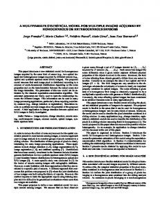
where c is the speed of light in the free space. Note also that PF S ∝ (r + r0 )−2 for any operating frequency and bandwidth. The overall transmission loss is computed by substituting (2) and (6) into (8). The reflection loss `R at S can be calculated in a similar form with (1) by simply changing ψ into π2 − ψ21 as can be seen from Fig. 1. 2.3. Scatterer Distribution Let the x-y coordinate system be defined such that the Tx is at the origin and the Rx lies on the x axis, as depicted in Fig. 2. In traditional

Figure 2. Angular displacement θ(x, y) between OR (x, y) and Ok (or O⊥ ).

Progress In Electromagnetics Research B, Vol. 17, 2009

195

RT simulations [14–18], the reflecting elements are perfectly planar with finer details of the surfaces being ignored. Subsequently, as mentioned in Section 2.1, in the ideal case of only two strip orientations Ok and O⊥ existing in the indoor environment, the distribution function of scattering elements with coordinates (x, y) has nonzero value only at certain x and y. Here, (x, y) refers to the coordinate of the strip center. In other words, suppose that OR (x, y) is the required strip direction at (x, y) such that the law of specular reflection can be complied with as pictured in Fig. 2. ©The pdfªof scatterer distribution, fx,y (x, y) 6= 0 if and only if OR ∈ Ok , O⊥ . Nevertheless, in reallife environments, more irregularly shaped scatterers such as furniture, door frames, and window casings will likely lead to “non-parallel” or “non-perpendicular” structures. Even if these effects are secondary, surface ruggedness of the walls and partitions will give rise to nonspecular reflections. In order to facilitate such non-ideal scenarios, we assume that fx,y (x, y) is continuous in the x-y space and is dependent on the angular displacement θ(x, y) between Ok (or O⊥ ) and OR (x, y) as shown in Fig. 2. There are a variety of angular distribution functions discussed in the computer graphics literature [25, 26], which attempt to characterize the distribution of the angle between the direction of the a posteriori mean surface (i.e., Ok or O⊥ ) and the predicted direction of the local reflecting surface defined as the bisector of the wave-source direction and the viewing direction (i.e., OR ). The Beckmann distribution for rough surfaces has been discussed in [25, 26], which is given by ½ ¾ 1 tan2 θ fθ (θ) ∝ exp − 2 (10) cos4 θ ΛB where ΛB is a parameter controling the angular shape of the distribution. One of the problems with the Beckmann distribution is that the shape is critically dependent on the width parameter ΛB [25, 26]. When ΛB is small, the pdf profile is highly collimated around an angular spike at θ = 0◦ . When ΛB is large then there are two angular side lobes [25, 26]. Here we are mainly interested in modeling the angular shape of the spike, where the pdf fθ (θ) should decrease monotonically as the angular displacement increases. To simplify the control of the pdf, we have followed the similar methodology in [25, 26] and used a small angle approximation to the Beckmann distribution, which yields a Gaussian pdf ½ ¾ sin2 θ fθ (θ) ∝ exp − (11) 2Λ2 The angle spreading factor Λ is controlled by the orientation

196

Chen et al.

randomness of the objects in the indoor environment. It is worth emphasizing that the Gaussian pdf underpinning the models in (11) and [25, 26] has a single parameter and maintains the same shape for all parameter settings. Because a smaller value of fθ (θ) signifies a lower probability of existence of the predicted reflecting surface, it is conjectured that the scatterer distribution fx,y (x, y)∝fθ (θ(x, y)). By inspecting Fig. 2, θ can be expressed as ( 0 if the reference orientation is Ok θk = ψ−ψ 2 , (12) ψ−ψ 0 π θ⊥ = 2 − 2 , if the reference orientation is O⊥ If the two directions are equally probable, the pdf of the scatterer

(a)

(b)

Figure 3. Scatterer distributions with (a) Λ = 0.1 and (b) Λ = 0.4. The locations of Tx and Rx are marked with “×” and “◦”, respectively.

Progress In Electromagnetics Research B, Vol. 17, 2009

197

distribution can be obtained as ( ( £ ¤) ½ ¾) sin2 θk (x, y) 1 1 sin2 [θ⊥ (x, y)] fx,y (x, y) = κ exp − + exp − (13) 2 2Λ2 2 2Λ2 RR where κ is a normalization constant to ensure that fx,y (x, y)dxdy = 1. Fig. 3 illustrates the scatterer distribution within a 40 m × 40 m service region for two continuous channels with different spreading factors. The Tx and Rx are located at (−5 m, 0 m) and (5 m, 0 m), respectively. Two important observations can be made from Fig. 3. First, as we increase the value of Λ the channel is “smoothed” and the scatterers are more homogeneously distributed in the service region, which corresponds to the scenario when the surface orientation becomes more irregular. Second, multiple scattering clusters, each representing a group of multipath components showing similar AOA, AOD, and delay, are naturally formed through (13). This phenomenon agrees well with the clustered propagation paths observed in the indoor experiment [19, 20, 22, 27]. © It isªworth noting that by relaxing the requirement that OR ∈ Ok , O⊥ , the analysis in Section 2.1 for the derivation of `T,T x→S and `T,S→Rx is only an approximation, where the transmission loss caused by “non-parallel” or “non-perpendicular” scatterers is neglected. Nevertheless, this simplification could be justified by considering that the majority of OR are highly concentrated around Ok or O⊥ in a normal building as suggested in (13). Subsequently, the joint pdf fr,ψ (r, ψ) is found by applying the Jacobian transformation as fr,ψ (r, ψ) = |r|fx,y (r cos(ψ − ψ0 ), r sin(ψ − ψ0 ))

(14)

The next step is to find a relationship between the total path propagation delay τ and the azimuth ψ, which is given by p r + r2 + D2 − 2rD cos(ψ − ψ0 ) r + r0 τ= = (15) c c The relationship between r and the delay τ can be found from (15) as r = h(τ, ψ) =

D2 − τ 2 c2 2 [D cos(ψ − ψ0 ) − τ c]

(16)

The joint delay-azimuth pdf is given by ¯ fr,ψ (r, ψ) ¯¯ fτ,ψ (τ, ψ) = |J(r, ψ)| ¯r=h(τ,ψ)

(17)

198

Chen et al.

where J(r, ψ) is the Jacobian transformation ¯ ¯−1 ¯ ∂r ¯ 2 (D cos(ψ − ψ0 ) − τ c)2 J(r, ψ) = ¯¯ ¯¯ = 2 ∂τ D c + τ 2 c3 − 2τ c2 D cos(ψ − ψ0 )

(18)

Substituting (13), (14), (16), and (18) into (17) yields ¡ 2 ¢¡ ¢ D − τ 2 c2 D2 c + τ 2 c3 − 2τ c2 D cos(ψ − ψ0 ) fτ,ψ (τ, ψ) = 4 (D cos (ψ − ψ0 ) − τ c)3 ( ( £ ¤) ½ ¾) sin2 θk (x, y) 1 sin2 [θ⊥ (x, y)] 1 ×κ exp − + exp − (19) 2 2Λ2 2 2Λ2 Equation (19) gives the joint delay-azimuth pdf observed at the Tx where the azimuth angle is measured relative to a wall of the building. 2.4. PAS and PDS Following from the definition in [28], the PAS at the Tx is easily derived as fp (ψ) = Σψ Pψ (ψ) Z ∞ = Σψ PR (τ, ψ)fτ,ψ (τ, ψ)dτ D

Z c∞ = Σψ

D c

PR (r, ψ)|r=h(τ,ψ) ·fτ,ψ (τ, ψ)dτ

(20)

where Σψ is a normalization factor to ensure that fp (ψ) is a pdf and Pψ (ψ) is the mean power of outgoing waves with AOD ψ. Substituting (8), (16), and (19) into (20) yields the final result for the PAS. In a similar manner, the PDS can be evaluated as fp (τ ) = Στ Pτ (τ ) Z 2π = Στ PR (τ, ψ)fτ,ψ (τ, ψ)dψ 0 Z 2π = Στ PR (r, ψ)|r=h(τ,ψ) ·fτ,ψ (τ, ψ)dψ

(21)

0

where Στ is a normalization constant to ensure that fp (τ ) is a pdf and Pτ (τ ) is the average power of signal with time-of-arrival (TOA) τ .

Progress In Electromagnetics Research B, Vol. 17, 2009

199

Figure 4. Pictorial illustration of the multiple-reflection process. 2.5. Extending the Analysis to Multiple-reflection Scenarios We will now extend the preceding analysis to a more general situation with multiple-reflection process. Fig. 4 shows the geometry and notation used to derive the PAS and PDS of the scattering models. For simplicity, we consider a double-reflection process where S1 and ~1 and S ~2 , respectively. Other S2 are reflectors with position vectors S model parameters are defined as follows (see also Fig. 4): • • • • • •

r1 : The distance of separation between Tx and S1 ; r10 : The distance of separation between S1 and Rx; r2 : The distance of separation between S1 and S2 ; r20 : The distance of separation between S2 and Rx; D: The distance of separation between Tx and Rx; ψ0 : The angle of the direct path between Tx and Rx referenced to an exterior wall; • ψ1 : The angle of the Tx-S1 path referenced to an exterior wall; • ψ2 : The angle of the S1 -S2 path referenced to an exterior wall; • τ2 : The path delay for signal traveling from S1 to Rx; • τ : The total propagation delay for signal traveling from Tx to Rx via S1 and S2 . ³ ´ ~1 The distribution of S1 is characterized by fS~1 S = fr1 ,ψ1 (r1 , ψ1 ), which is derived in a similar manner with (13) and (14)

200

Chen et al.

by noting that only the paths close to the S1 -to-Rx are predominant. Therefore, the relevant angular displacement θ (see also (12)) that determines fr1 ,ψ1 (r1 , ψ1 ) is the angle between Ok (or O⊥ ) and the ³ ´ ~1 defined by the Tx-S1 and S1 -Rx paths (cf. Fig. 2). actual OR S Essentially, we have simplified the discussion by assuming that the distribution of S1 is independent of the location of S2 . Subsequently, the scatterer distribution of S2 conditioned on S1 is characterized by ³ ´ ~2 |S ~1 = fτ ,ψ |r ,ψ (τ2 , ψ2 |r1 , ψ1 ) fS~2 |S~1 S (22) 2 2 1 1 which can be derived in a similar way with (19), given (r1 , ψ1 ). Following from Section 2.2, the mean power received at the Rx for the ray-path Tx-S1 -S2 -Rx is given by PR (r1 , ψ1 , τ2 , ψ2 ) = PF S × `T,T x→S1 × `T,S1 →S2 ×`T,S2 →Rx × `R,T x→S1 →S2 × `R,S1 →S2 →Rx (23) where PF S denotes the free space path-loss and is proportional to (r1 + r2 +r20 )−2 . `T,T x→S1 , `T,S1 →S2 and `T,S2 →Rx represent, respectively, the transmission loss associated with the Tx-S1 , S1 -S2 , and S2 -Rx path trajectories. `R,T x→S1 →S2 and `R,S1 →S2 →Rx are the reflection loss due to reradiation from S1 and S2 , respectively. All the terms in (23) can be calculated by following the same procedures in Sections 2.1 and 2.2. Finally, the average power of outgoing wave with AOD ψ1 is given by Z Z Z (2) Pψ1 (ψ1 ) = PR (r1 , ψ1 , τ2 , ψ2 )fr1 ,ψ1 ,τ2 ,ψ2 (r1 , ψ1 , τ2 , ψ2 )dψ2 dτ2 dr1 r1 τ2 ψ2 Z Z Z = PR (r1 , ψ1 , τ2 , ψ2 )fτ2 ,ψ2 |r1 ,ψ1 (τ2 , ψ2 |r1 , ψ1 ) r1

τ2

ψ2

fr1 ,ψ1 (r1 , ψ1 )dψ2 dτ2 dr1

(24)

where the superscript (2) indicates a double-reflection propagation process. The overall PAS is calculated using h i (1) (2) fp (ψ1 ) = Σψ1 Pψ1 (ψ1 ) + Pψ1 (ψ1 ) (25) (1)

where Pψ1 (ψ1 ) refers to the mean power of departing wave with AOD ψ1 when it undergoes a single reflection. Σψ1 is a normalization factor to ensure that fp (ψ1 ) is a pdf.

Progress In Electromagnetics Research B, Vol. 17, 2009

201

Next, the average power of signal with TOA τ when it undergoes a double-reradiation is given by Z Z Z £ Pτ(2) (τ ) = PR (r1 , ψ1 , τ2 , ψ2 ) r1 ψ1 ψ2 ¯ ¤¯ fr1 ,ψ1 ,τ2 ,ψ2 (r1 , ψ1 , τ2 , ψ2 ) ¯¯ dψ2 dψ1 dr1 Z Z =

τ2 =τ −

Z

r1 c

£ PR (r1 , ψ1 , τ2 , ψ2 )fτ2 ,ψ2 |r1 ,ψ1 (τ2 , ψ2 |r1 , ψ1 ) r1 ψ1 ψ2 ¯ ¤¯ fr1 ,ψ1 (r1 , ψ1 ) ¯¯ dψ2 dψ1 dr1 (26) r1 τ2 =τ −

c

The overall PDS is obtained as i h fp (τ ) = Στ Pτ(1) (τ ) + Pτ(2) (τ )

(27)

(1)

In (27), Pτ (τ ) refers to the mean power of signal with TOA τ when it undergoes a single reflection, and Στ is a normalization constant. With a similar approach, the analysis can be easily extended to propagation process with higher-order reflections. Nevertheless, the above derivations involve multifold integrals, which are computationally intensive and inconvenient for numerical evaluation. To simplify the analysis, we assume that the multiplereflection process from Tx to Rx can be approximated using an equivalent virtual path that involves a single specular reflection at S1 , which yields the same AOA at the Rx [12]. Apparently, multiple-reflection broadens the channel impulse response for radiowave propagation from S1 to Rx from a delta function to a graduallydecaying function with a finite temporal support. Furthermore, indoor channel measurements suggest that the correlation of the delay spread with the distance is insignificant. Effectively, they may be considered to be independent [29, 30]. Consequently, the empirical observation prompts the following conjecture: The virtual path has an extended propagation distance r1 + r10 + ∆r, where ∆r is a constant (see Fig. 4). Accordingly, the total path propagation delay is derived as µ ¶ q r1 +r10 +∆r 1 2 2 τ= = r1 + D +r1 −2r1 Dcos(ψ1 −ψ0 )+∆r (28) c c Squaring both sides of (28) and solving for r1 yields r1 = h1 (τ, ψ1 ) =

D2 − (τ c − ∆r)2 2 [D cos(ψ − ψ0 ) − (τ c − ∆r)]

(29)

202

Chen et al.

Following from the same derivations in (17)–(19), the joint delayazimuth pdf becomes

=

fτ,ψ1 (τ, ψ1 ) ¤£ £ 2 ¤ D −(τ c−∆r)2 D2 c+(τ c−∆r)2 c−2(τ c−∆r)cDcos(ψ1 −ψ0) ( ×κ

4 [D cos(ψ1 − ψ0 ) − (τ c − ∆r)]3 £ ¤) ¾) ½ sin2 θk (x, y) 1 sin2 [θ⊥ (x, y)] 1 exp − (30) + exp − 2 2Λ2 2 2Λ2 (

Finally, the PAS and PDS are obtained by substituting (30) into (20) and (21). Note that both the transmission loss from S1 to Rx and the free space path-loss have to take into account the additional loss introduced by ∆r. 3. NUMERICAL EXAMPLES In this section, the theoretical single-channel-trial and multiplechannel-trial PAS will be compared against the measured angle power profile in [19] and the RT solutions in [18], respectively. Moreover, the influence of the model parameters on the behaviors of PAS and PDS will be studied as well. 3.1. Angle Statistics in a Single Channel Trial: Comparison with the Empirical Data We first explore the behaviors of path-angle profiles from a single channel trial. The conductivity of each scattering strip is 0.02 S/m and the relative permittivity is 6, which fall in the range of the constitutive parameters of concrete within 3–24 GHz [31]. The penetration loss is assumed to be 15 dB for concrete walls [32]. The above parameters generally concur with the measurement environment in [19]. The following values are selected to best fit the measured PAS in [19]. The density of the strips is ζ = 18 m−2 , the average length of the strip is L = 6 m, the spreading factor in (13) is Λ = 0.1, the Tx-to-Rx distance is D = 10 m, and the building-referenced direct-path angle is ψ0 = 40◦ . Two critical observations can be made from Fig. 5. First, multiple clusters that are resolvable in the angular domain are observed. This phenomenon is caused by the scatterer distribution formulated in (13) (see also Fig. 3), which shows good agreement with the observed clustered propagation paths in the indoor environment [19, 22, 27]. Second, Cluster 1 is nonsymmetric while Clusters 2 and 3 are nearly symmetric. The asymmetry in the former case is different from

Progress In Electromagnetics Research B, Vol. 17, 2009

203

the symmetric, single-lobed Laplacian distribution and PAS patterns suggested by other geometric models [2, 9–13]. This lop-sidedness is due to the less random orientations of reflecting planes in a normal building, which has some confirmation from the measured non-line-ofsight (NLOS) PAS in [19]. In [19], a total of 5 NLOS data sets were collected in a town house and another 6 were recorded in a typical office environment. The frequency of measurement was from 2 to 8 GHz with resolution of 3.75 MHz. Each data set mimicked a measurement over a virtual array comprised of 20 elements. The channel was assumed to be static over the measuring interval. Averaging over all the measurements gave the average PAS, which offset the effect of asymmetry PAS shape for a specific realization of the multipaths. The experimental data in [19] are compared to the theoretical data of Cluster-1 angle power spectrum in Fig. 5, which demonstrates interesting resemblance between these two sets of data. Specifically, substantial side lobes along the angular axis and deep nulls in between the lobes can be found for both the two sets of data. On the other hand, this empirical observation in [19] is in contrast to the outdoor NLOS experimental results in [28], collected in a macrocellular urban channel. These measurements were conducted at 1.8 GHz using an 8element uniform linear array at the base station with half-wavelength element spacing. The PAS has been estimated by using the SAGE

Figure 5. PAS for a single channel trial. Also shown is the comparison between the theoretical Cluster-1 PAS and the measured PAS in [19]. The empirical data in [19] have been normalized such that the overall power is the same as the power of Cluster 1. Encircled deep nulls in between the two side lobes are found for both the two sets of data.

204

Chen et al.

Figure 6. PAS for multiple-reflection scenarios with different ∆τ . algorithm. As illustrated in Fig. 4 of [28], the incident power is highly concentrated around the azimuth towards the mobile station, and has a nearly symmetric profile. We may thus infer that in a normal building, the proposed model could yield a better characterization of such irregularity as compared to other GCMs. Nevertheless, more experimental data are required to provide further justification for the above statements. Figure 6 depicts the influence of multiple reflections on the angle statistics. The model parameters are the same as the previous example except that a new variable ∆τ (∆τ = ∆r c , cf. Eqs. (28)–(30)) is introduced to approximate the multiple-bounce effect. Note that ∆τ is determined by the delay spread of the underlying multipath delay profile. It can be seen from Fig. 6 that multiple-reflection does not change the PAS remarkably for a wide range of ∆τ . One possible explanation is that the additional loss caused by ∆r for each multipath component is usually much smaller than the path loss in a singlereflection channel. Furthermore, the integration of the transmitted rays in the delay domain to obtain the PAS is an averaging/smoothing operation that effectively diminishes the multiple-reflection effect. In the subsequent discussions, we will focus on the single-reflection propagation process. 3.2. Angle Statistics in Multiple Channel Trials: Comparison with the RT Data To further establish the validity of the model, the theoretical PAS of multiple channel trials are collectively analyzed and the superimposed results are compared to the RT data reported in [18], which comprises 500 independent channel trials. Each trial is determined as follows.

Progress In Electromagnetics Research B, Vol. 17, 2009

205

First, the Tx location is selected at random within a boundary corresponding to the external wall of the building under investigation. The Rx location is then selected at random from the largest arc defined by the Tx-to-Rx distance. The profiles of path-angles from all 500 trials are summed to generate the overall profile. The RT program has been executed with two lattice building structures and with two real building databases. The two different lattice-building structures are distinguished by the number and size of their rooms. The sparselattice model has a larger interior-wall dimension and a smaller number of rooms as compared to the dense-lattice model. Furthermore, these two artificially-devised building structures also replicate the two real buildings, the Residential Laboratory (ResLab) on the Georgia Tech campus and the Georgia Centers for Advanced Telecommunications

(a)

(b)

Figure 7. Comparison between the theoretical results and the RT data collected in normal buildings [18]: (a) Sparse lattice and reslab, (b) dense lattice and GCATT.

206

Chen et al.

Technology (GCATT), respectively. The following numerical values are applied to derive the theoretical angular profiles. The conductivity is 0.003 S/m and the relative permittivity of reflecting surfaces is 4.5 following [18]. To resemble the sparse-lattice structure and the ResLab Building, the average length of the strip is set to be 3.92 m and the 2 −2 . On the other hand, the length and density of the strips is 3.92 2 m 2 −2 , respectively, density of the strips are set to be 7.84 m and 7.84 2 m for the dense-lattice model and the GCATT Building. In both cases, the Tx-to-Rx distance is 10 m, the spreading factor is 0.4 and the partition loss is 3.4 dB for light walls based on the COST231 multi-wall model [31]. A different value of penetration loss is used here because the interior of the real building databases in [18] is assumed to be plasterboard and wood walls. The combined profile using the proposed model is obtained as follows. With a fixed Tx, 180 Rx locations are evenly distributed on the circumference of the arc defined by the Txto-Rx distance. Subsequently, the PAS and PDS from all 180 trials are summed to give the collective profile. Figure 7 shows the comparison for the theoretical PAS obtained from (20) with the simulated data in [18]. It can be seen from Fig. 7 that deterministic angle clustering is clearly visible for both the theoretical and simulated results. The angles of the PAS nulls are 0, 90, 180, 270, and 360 degrees, and the mean angles of the clusters are 45, 135, 225, and 315 degrees regardless of the type of lattice or real building. Local minima in the signal power distribution at 0, 90, 180, 270, and 360 degrees are attributed to the transmission/reflection coefficients at these angles. Furthermore, the theoretical PAS predicts a comparable signal strength difference between peak and bottom with the RT solutions as can be seen from Fig. 7. It is worth emphasizing that if the conventional symmetric, single-lobed functions (e.g., Laplacian, Gaussian, or pdfs generated by other GCMs) are used to describe the angular power distribution in a single trial, the combined PAS would be a non-clustered, uniform distribution over the entire angular range. Therefore, the proposed model may be superior to the existing channel models when considering the signal propagation in a normal building. 3.3. Behaviors of PAS and PDS for Various Channel Model Parameters In this section, we explore the behaviors of PAS and PDS for various channel model parameters. Likewise the paths of multiple channel trials are superimposed and collectively analyzed. The series of examples are composed of four parts. First, we examine the influence

Progress In Electromagnetics Research B, Vol. 17, 2009

207

(a)

(b)

Figure 8. a) PAS and (b) PDS for Case Study 1. Angles are referenced to the exterior building wall. of the spreading factor, which is determined by the orientation randomness of the reflection plane (Case Study 1). In the second part, we consider the effect of different strip lengths on the channel properties (Case Study 2). In the third part, the density of the strips is used as the basis for the investigation (Case Study 3). Finally, we look into the influence of the Tx-to-Rx distance on the channel properties. Table 1 summarizes the parameters that are used in the four study cases. The obtained PAS and PDS for Case Study 1 are depicted in Fig. 8. Similar patterns have been found for all the other cases. Two shape parameters, namely the peak-to-null ratio γ and the decaying rate ν dB/ns, are used to characterize the PAS and PDS (see also Figs. 8(a)–(b)). Note that larger γ and |ν| also indicate smaller cluster angular spread and delay spread, respectively. The corresponding numerical results are listed in Table 1. It can be found that γ increases

208

Chen et al.

Table 1. Model parameters and numerical results for the four study cases. Case Study 1

Case Study 2

Case Study 3

Case Study 4

εr σ (S/m) fc (GHz) L (m) Λ ζ (m−2 ) D (m)

4.5 0.003 2.4 4 [0.1 0.2 0.4] 1/16 10

4.5 0.003 2.4 [4 10 20] 0.1 1/16 10

4.5 0.003 2.4 4 0.1 [1/32 1/16 1/8] 10

4.5 0.003 2.4 4 0.1 1/16 [6 10 20]

γ

9.614 (Λ = 0.1) 3.585 (Λ = 0.2) 2.180 (Λ = 0.4)

9.614 (L = 4) 15.958 (L = 10) 24.515 (L = 20)

6.277 (ζ = 1/32) 9.614 (ζ = 1/16) 14.095 (ζ = 1/8)

7.086 (D = 6) 9.614 (D = 10) 14.095 (D = 20)

v (dB/ns)

−0.36 (Λ = 0.1) −0.36 (Λ = 0.2) −0.36 (Λ = 0.4)

−0.36 (L = 4) −0.77 (L = 10) −1.44 (L = 20)

−0.21 (ζ = 1/32) −0.36 (ζ = 1/16) −0.63 (ζ = 1/8)

−0.42 (D = 6) −0.36 (D = 10) −0.32 (D = 20)

for a smaller Λ, larger L, larger ζ, and larger D. On the other hand, |ν| increases for a larger L, larger ζ, and smaller D. However, it seems that the spreading factor has very marginal influence on |ν|. In all cases, the PDS can be approximated by an exponential decaying function, which has been commonly observed in numerous measurement campaigns (see e.g., [19, 22, 27, 28]). Finally, as a practical concern, large values of γ suggest that antennas with nonadaptive directional beams that point toward the peaks of the clusters may enhance the performance of WPANs in a normal building. 4. CONCLUSIONS We have proposed a geometrically-based statistical model for radio propagation in rectangular office buildings, where the orientations of the reflecting planes are structured. The important channel parameters including PAS and PDS have been derived. The theoretical single-

Progress In Electromagnetics Research B, Vol. 17, 2009

209

trial PAS and multiple-trial PAS correctly replicate the asymmetric angular profile observed in [19] and the angle clustering reported in [18], respectively. Both these phenomena cannot be devised using the conventional statistical and geometric models. The PDS profiles exhibit an exponential distribution, which agrees well with the empirical observations made in the existing literature [19, 22, 27, 28]. The results would provide an insight into the design and evaluation of WPANs in buildings of this type. The following open issues should be addressed in future to facilitate a realistic implementation of the proposed analytical framework: (i) Ascertaining the range of applicability of the current model by using more empirical data; and (ii) optimizing model parameters for different rectangular buildings through comprehensive measurement campaigns. REFERENCES 1. Molisch, A., D. Cassioli, C.-C. Chong, S. Emami, A. Fort, B. Kannan, J. Karedal, J. Kunisch, H. G. Schantz, K. Siwiak, and M. Z. Win, “A comprehensive standardized model for ultrawideband propagation channel,” IEEE Trans. Antennas Propagat., Vol. 54, 3151–3166, Nov. 2006. 2. Molisch, A., H. Asplund, R. Heddergott, M. Steinbauer, and T. Zwick, “The COST259 directional channel model — Part I: Overview and methodology,” IEEE Trans. Wirel. Commun., Vol. 5, 3421–3433, Dec. 2006. 3. Franceschetti, M., “Stochastic rays pulse propagation,” IEEE Trans. Antennas Propagat., Vol. 52, 2742–2752, Oct. 2004. 4. Martini, A., M. Franceschetti, and A. Massa, “Stochastic ray propagation in stratified random lattices,” IEEE Antennas Wirel. Propagat. Lett., Vol. 6, 232–235, 2007. 5. Hu, L. Q., H. Yu, and Y. Chen, “Path loss models based on stochastic rays,” IET Micro. Antennas Propag., Vol. 1, No. 3, 602–608, 2007. 6. Hansen, J. and M. Reitzner, “Efficient indoor radio channel modeling based on integral geometry,” IEEE Trans. Antennas Propagat., Vol. 52, 2456–2463, Sep. 2004. 7. Ullmo, D. and H. U. Baranger, “Wireless propagation in buildings: A statistical scattering approach,” IEEE Trans. Veh. Technol., Vol. 47, No. 9, 947–955, 1999. 8. Janaswamy, R., “An indoor pathloss model at 60 GHz based on transport theory,” IEEE Antennas Wirel. Propagat. Lett., Vol. 5, 58–60, 2006.

210

Chen et al.

9. Janaswamy, R., “Angle and time of arrival statistics for the Gaussian scatter density model,” IEEE Trans. Wirel. Commun., Vol. 1, 488–497, Jul. 2002. 10. Petrus, P., J. H. Reed, and T. S. Rappaport, “Geometrical-based statistical macrocell channel model for mobile environments,” IEEE Trans. Commun., Vol. 50, 495–502, Mar. 2002. 11. Chen, Y. and V. K. Dubey, “Accuracy of geometric channelmodeling methods,” IEEE Trans. Veh. Technol., Vol. 53, 82–93, Jan. 2004. 12. Molisch, A. F., “A generic model for MIMO wireless propagation channels in macro- and microcells,” IEEE Trans. Signal Processing, Vol. 52, 61–71, Jan. 2004. 13. Hamalainen, J., S. Savolainen, R. Wichman, K. Ruotsalainen, and J. Ylitalo, “On the solution of scatter density in geometry based channel models,” IEEE Trans. Wirel. Commun., Vol. 6, No. 3, 1054–1062, Mar. 2007. 14. Iskander, M. F. and Z. Yun, “Propagation prediction models for wireless communication systems,” IEEE Trans. Microw. Theory Tech., Vol. 50, 662–673, Mar. 2002. 15. Seidel, S. Y. and T. S. Rappaport, “Site-specific propagation prediction for wireless in-building personal communication system design,” IEEE Trans. Veh. Technol., Vol. 43, 879–891, Nov. 1994. 16. Hassan-Ali, M. and K. Pahlavan, “A new statistical model for site-specific indoor radio propagation prediction based on geometric optics and geometric probability,” IEEE Trans. Wireless Commun., Vol. 1, 112–124, Jan. 2002. 17. Fortune, S., D. Gay, B. Kernighan, O. Landron, R. Valenzuela, and M. Wright, “WISE design of indoor wireless systems: Practical computation and optimization,” IEEE Comput. Sci. Eng., Vol. 2, 58–69, Spring, 1995. 18. Jo, J. H., M. A. Ingram, and N. Jayant, “Deterministic angle clustering in rectangular buildings based on ray-tracing,” IEEE Trans. Commun., Vol. 53, 1047–1052, Jun. 2005. 19. Poon, A. and M. Ho, “Indoor multiple-antenna channel characterization from 2 to 8 GHz,” Proc. IEEE ICC, Anchorage, AK , 3519–3523, May 2003. 20. Zhang, Y., A. K. Brown, W. Q. Malik, and D. J. Edwards, “High resolution 3-D angle of arrival determination for indoor UWB multipath propagation,” IEEE Trans. Wirel. Commun., Vol. 7, 3047–3055, Aug. 2008. 21. Malik, W. Q., C. J. Stevens, and D. J. Edwards, “Spatio-

Progress In Electromagnetics Research B, Vol. 17, 2009

22.

23. 24. 25. 26. 27. 28.

29.

30. 31. 32. 33.

211

temporal ultrawideband indoor propagation modelling by reduced complexity geometric optics,” IET Commun., Vol. 1, No. 4, 751– 759, 2007. Spencer, Q. H., B. Jeffs, M. A. Jensen, and A. L. Swindlehurst, “Modeling the statistical time and angle of arrival characteristics of an indoor multipath channel,” IEEE J. Select. Areas Commun., Vol. 18, No. 3, 347–360, 2000. Bertoni, H., W. Honcharenko, L. R. Maciel, and H. Xia, “UHF propagation prediction for wireless personal communications,” Proc. IEEE , Vol. 82, 1333–1359, Sep. 1994. Ghavami, M., L. B. Michael, and R. Kohno, Ultra Wideband Signals and Systems in Communication Engineering, John Wiley and Sons, 2004. Healey, G. H. and T. O. Binford, “Local shape from specularity,” Computer Vision, Graphics, and Image Processing, Vol. 42, No. 1, 62–86, 1988. Ragheb, H. and E. R. Hancock, “A probabilistic framework for specular shape-from-shading,” Pattern Recognition, Vol. 36, 407– 427, 2003. Cramer, R. J.-M., R. A. Scholtz, and M. Z. Win, “Evaluation of an ultra-wide-band propagation channel,” IEEE Trans. Antenna Propagat., Vol. 50, No. 5, 561–570, 2002. Pedersen, K., P. Mogensen, and B. Fleury, “A stochastic model of the temporal and azimuthal dispersion seen at the base station in outdoor propagation environments,” IEEE Trans. Veh. Technol., Vol. 49, 437–447, Mar. 2000. Cassioli, D., M. Z. Win, and A. F. Molisch, “The ultrawide bandwidth indoor channel: From statistical model to simulations,” IEEE J. Select. Areas Commun., Vol. 20, 1247–1257, Aug. 2002. McDonnell, J. T. E., T. P. Spiller, and T. A. Wilkinson, “RMS delay spread in indoor LOS environments at 5.2 GHz,” IEE Electronics Letters, Vol. 34, 1149–1150, May 1998. Saunders, S. R. and A. Arag´on-Zavala, Antennas and Propagation for Wireless Communication Systems, 2nd edition, John Wiley and Sons, Chichester, West Sussex, England, 2007. Rappaport, T., Wireless Communications: Principles and Practice, 2nd edition, Prentice Hall PTR, 2001. Sedaghat Alvar, N., A. Ghorbani, and H. R. Amindavar, “A novel hybrid approach to ray tracing acceleration based on preprocessing & bounding volumes,” Progress In Electromagnetics

212

Chen et al.

Research, PIER 82, 19–32, 2008. 34. Cocheril, Y. and R. Vauzelle, “A new ray-tracing based wave propagation model including rough surfaces scattering,” Progress In Electromagnetics Research, PIER 75, 357–381, 2007.