This article has been accepted for publication in a future issue of this journal, but has not been fully edited. Content may change prior to final publication. Citation information: DOI 10.1109/ACCESS.2018.2807698, IEEE Access
1
Glioma Segmentation Using a Novel Unified Algorithm in Multimodal MRI Images Qingneng Li, Zhifan Gao*, Member, IEEE, Qiuyu Wang, Jun Xia, Heye Zhang, Member, IEEE, Huailing Zhang, Huafeng Liu and Shuo Li
Abstract—To achieve the better segmentation performance, we propose a unified algorithm for automatic glioma segmentation. In this paper, we firstly use spatial fuzzy c-mean clustering to estimate region-of-interest in multimodal MRI images, and then extract some seed points from there for region growing based on a new notion “affinity”. In the end, we design a two-step strategy to refine the glioma border with region merging and improved distance regularization level set method. In BRATS 2015 training database, we evaluate the accuracy and robustness of our method with performance scores, including Dice, Positive Predictive Value (PPV), Sensitivity, Hausdorff distance (HD) and Euclidean distance (ED). The high metric values (Dice=0.86, PPV=0.90 and Sensitivity=0.84) and small distance errors (HD=14.39mm and ED=3.31mm) indicate a remarkable accuracy. Also, we observe the ranking is No.1 in Dice and PPV by comparison with the state-of-the-art methods. In addition, the robustness is also at a high level due to the refinement structure. And Spearman’s rank coefficient test verities a significant correlation between the high grade gliomas and low grade gliomas. Overall, the proposed method is effective in segmenting gliomas in multimodal images and Flair images, and has the potential in routine examinations of gliomas in daily clinical practice. Index Terms—Distance regularized level set evolution, region growing based on affinity, spatial fuzzy c-mean clustering, unified algorithm.
I. INTRODUCTION
G
LIOMAS are
the most common and malignant brain tumors with the short life expectancy [1]. Only 5% patients
This work was supported by the Project funded by China Postdoctoral Science Foundation (2017M620394). (Corresponding author: Zhifan Gao ) Qingneng Li is with Sino-Dutch Biomedical and Information Engineering School, Northeastern University, Shenyang 110819, China, and also with Shenzhen Institutes of Advanced Technology, Chinese Academy of Sciences, Shenzhen 518055, China (e-mail:
[email protected]) Zhifan Gao and Heye Zhang are with Shenzhen Institutes of Advanced Technology, Chinese Academy of Sciences, Shenzhen 518055, China (e-mail: {zf.gao, hy.zhang}@siat.ac.cn) Qiuyu Wang and Jun Xia are with Department of Radiology, Shenzhen Second People's Hospital, Shenzhen 518035, China (e-mail:
[email protected],
[email protected]) Huailing Zhang is with Information Engineering School, Guangzhou Medical University, Guangzhou 524023,China (e-mail:
[email protected]) Huafeng Liu is with the State Key Laboratory of Modern Optical Instrumentation, Department of Optical Engineering, Zhejiang University, Hangzhou 310027, China (e-mail:
[email protected]). Shuo Li is with University of Western Ontario, London, N6A 3K7, Canada (e-mail:
[email protected])
suffering glioblastoma (GBM) survive more than five years after diagnosis [1], [2]. It is the severity and popularity that make glioma segmentation become one of the crucial procedures in surgery and treatment. Up to now, glioma segmentation in clinical tumor images is mostly performed manually. However, manual delineation is time-consuming and depends on the individual operator [3]. Thus, a semi-automatic or automatic glioma segmentation method is demanded greatly to assist the glioma diagnosis [3],[4]. Nevertheless, glioma segmentation is given many difficulties by isointense (the same signal intensity as that of brain tissues), hypointense (darker than brain tissues) property of gliomas, and fuzziness of tumor margins [5]. Furthermore, structures of tumor are varied in different patients in terms of size, extension, and localization. It prohibits the strong priors from being applied in shape and location that are important to segment many other anatomical structures [6]. Finally, artifacts and noise in MRI images also increase the difficulty in segmentation of gliomas [3] Many imaging techniques have been applied to examine tumor-induced tissue changes. For instance, multimodal MRI images have been used frequently by radiologists in segmenting brain tumor images because multimodal MRI images can provide various data, and reveal different parts on tumors [3]. Although segmentation of gliomas from the brain makes a little progress, it is still a challenging task. A. Related Work Many glioma segmentation algorithms have been developed based on different kinds of pathology properties. We can mainly categorize these glioma segmentation methods into two groups: probability-based methods and non-probability-based methods. In probability-based methods, discriminative methods directly learn the relationship between specific (local) image features and segmentation labels without any domain knowledge [6], such as support vector machines [7] or decision trees [8]. Nevertheless, they depend explicitly on intensity features, restricting their segmentation in the same imaging protocol used for the training data. Apart from being time consuming, a great deal of training data is desired for discriminative model to find the relationship. Generative methods as the other probability-based methods build the probability models based on pixel labels and intensities. After specifying a full probabilistic model, these methods compute the class conditional likelihood and prior probability functions of the labels in order to simulate or generate all variables [9], e.g. Markov Random Fields (MRF)
2169-3536 (c) 2018 IEEE. Translations and content mining are permitted for academic research only. Personal use is also permitted, but republication/redistribution requires IEEE permission. See http://www.ieee.org/publications_standards/publications/rights/index.html for more information.
This article has been accepted for publication in a future issue of this journal, but has not been fully edited. Content may change prior to final publication. Citation information: DOI 10.1109/ACCESS.2018.2807698, IEEE Access
2 [10]. However, generative methods demand strong prior knowledge to calculate their probability function, for indicating their downsides in segmenting gliomas. By contrast, non-probability-based methods have a big advantage that they can complete the segmentation works quite fast. Moreover, these methods have a capacity to segment gliomas automatically and have fewer requirements for the dataset. For example, fuzzy c-means (FCM) algorithm was presented for automatic glioma segmentation, exacting highly similar point as a same class, but it only considered intensity similarity in lack of extra constraints [11]. Besides, many versions of seeded region growing algorithms were also put forwards in various medical image segmentations [12-14]. Afterwards, active contour models, like snake [15] and level set method [16-19] began to be widely used. However, both region growing methods and active contour models required to initialize seed points or contours. Often their segmentations were not exact when the initializations were inappropriate. It was the poor constraint conditions and manual interventions that limited their success on the larger number of data set, indicating that a more sophisticated method was being desired urgently. B. Our Contributions In this study, we develop a unified algorithm (refer as to UAGS) to detect the glioma border in brain MRI images. It comprises three components: the spatial fuzzy c-mean (SFCM) algorithm, a new region growing method, and an improved distance regularized level set evolution (DRLSE) method. The main contributions of UAGS include: 1) Estimate region-of-interest with less pseudo lesions We estimate region-of-interest (ROI) using the SFCM algorithm. Here, a good ROI should be covered by the whole tumor without any non-tumor regions. However, the estimation may produce pseudo glioma regions (PGR) if based on mono-modal (i.e. one of four MRI sequences) images, since some brain tissues with the same intensity as gliomas might be misclassified as lesions, e.g., the cerebrospinal fluid (CSF). In fact, both Flair and T2 images highlight the whole tumor (See Figure 1). Therefore, we can use the multimodal images simultaneously for SFCM clustering, and then make an intersection with their results to remove parts of PGR. Furthermore, we train support vector machine (SVM) to automatically select the appropriate clustering result. In addition, the clustering results are also considered to generate a synthetic image that reinforces the glioma region and excludes the CSF for the following work. 2) Detect the entire glioma regions We intend to detect the entire glioma regions, even if there is more than one tumor settlement after diffusing. Thereby, we extract centroids of isolated regions and some points surrounding them as initial seeds, rather than high intensity pixels over a threshold. Furthermore, each of initial seeds, rather than their combination should start to grow iteratively with loose region growing criteria to ensure the entire glioma detection. Moreover, we propose a new region growing mechanism with the notion “affinity” capturing the idea of
Fig. 1. Manual annotation provided by the BRATS 2015 database. The tumor structures of edema (yellow), non-enhancing core (red), necrotic core (green) and enhancing core (cyan) can be respectively gained from Flair, T2 and T1c images from left to right. The whole tumor is shown at right.
nearness in location and similarity between their gray scale values [20]. In mathematics, affinity measurement can effectively capture the similarity between any two pixels [21]. 3) Refine the final glioma border Actually, many PGR may be produced in the process of the region growing if the wrong seed points are selected. To prevent this trouble, we design a two-step strategy as post processing to refine the final glioma regions with other constraint conditions or regularization. Firstly, for the large mass in there, we can make use of some criteria, like the Minimum Description Length (MDL) criteria to merge the isolated object regions such as to remove the PGR resulting from the bad seeds’ growth [22]. Secondly, we utilize improved DRLSE method to smooth the glioma border and eliminate small spots as well as slim piecewise curves II. METHODOLOGY Our UAGS method firstly uses SFCM clustering [18] with the SVM selection to estimate the ROI. Next, it starts region growth based on the notion “affinity” (RGBA) to detect the glioma region [20]. This new region growing method extracts seed points in terms of the location information of ROI rather than its intensity features. Then a two-step strategy is designed to refine the glioma regions because many PGR are introduced after region growing. Region merging based on MDL criteria is given priority to separate those non-tumor regions [22]. Finally, the glioma borders are smoothed with improved DRLSE method [16]. The flowchart of our method is illustrated in Figure 2. A. Region of interest estimation We should estimate ROI using the multimodal images (i.e. T2 and Flair images) simultaneously. The classical FCM algorithm is considered for brain tumor segmentation as physiological tissues are usually not homogeneous. Its objective function is defined as: 2
𝑠𝑠 (1) 𝐽 = ∑𝑘𝑖=1 ∑𝑁 𝑗=1 𝜇𝜇𝑖𝑗 �𝑥𝑗 − 𝑐𝑐𝑖 � where 𝑥 is one of total 𝑁 image pixels, 𝑘𝑘 equals the number of clusters, and ‖∙‖ denotes the Euclidean norm. The membership function 𝜇𝜇 and the centroids of cluster 𝑐𝑐 can be updated iteratively as follows:
𝜇𝜇𝑖𝑗 =
2
�𝑥 −𝑠𝑠 � 1−𝑚 ∑𝑘𝑛=1 � 𝑗 𝑖 � �𝑥 −𝑠𝑠 � 𝑗
𝑛
(2)
2169-3536 (c) 2018 IEEE. Translations and content mining are permitted for academic research only. Personal use is also permitted, but republication/redistribution requires IEEE permission. See http://www.ieee.org/publications_standards/publications/rights/index.html for more information.
This article has been accepted for publication in a future issue of this journal, but has not been fully edited. Content may change prior to final publication. Citation information: DOI 10.1109/ACCESS.2018.2807698, IEEE Access
3 𝑝
𝑞
𝑝
𝑞
′ = 𝜇𝜇𝑖𝑗 ℎ𝑖𝑗 �∑𝑘𝑛=1 𝜇𝜇𝑛𝑗 ℎ𝑛𝑗 (4) 𝜇𝜇𝑖𝑗 where 𝑝𝑝 and 𝑞𝑞 are two exponents controlling the respective base function. The variable ℎ𝑖𝑗 represents the spatial information and formulates as: ℎ𝑖𝑗 = ∑𝑛∈𝑁𝑗 𝜇𝜇𝑛𝑗 (5)
where 𝑁𝑗 is a local window centered on the image pixel 𝑗 and 𝑛𝑛 is the element of the window. The membership function 𝜇𝜇 and the centroid 𝑐𝑐 are updated as usual. According to (4) and (5), we apply this SFCM clustering algorithm in both Flair and T2 images. To automatically select the appropriate clustering result, SVM supervision should be taken into account. We extract some texture features and intensity features from patient image for training. Ultimately, we make an intersection with the selected clustering results of Flair and T2 images as the ROI
Fig. 2. The flowchart of our method. ROI: Region-of-interest; SFCM: Spatial fuzzy C-means algorithm; MDL: Minimum description length; DRLSE: distance regularization level set evolution.
𝑐𝑐𝑖 =
𝑚 ∑𝑁 𝑗=1 𝜇𝑖𝑗 𝑥𝑗 𝑚 ∑𝑁 𝑗=1 𝜇𝑖𝑗
(3)
where 𝑚 > 1 is fuzzy partition matrix exponent for controlling the degree of fuzzy overlap. Although the standard FCM algorithm is justifiable for fast medical image segmentation, it cannot exclude the image noise and artifacts in the lack of spatial information [18]. Often people utilize morphological operations as simple spatial restrictions at the post-processing stage [17]. Chuang et.al [23] incorporated spatial information into fuzzy membership function directly. The new membership function is modified as:
B. Glioma detection The region growing method is an iterative image segmentation method with three elementary parts: seed points selection, definition of similarity, and criteria for convergence to terminate the iterative process [14]. The initial region begins as the exact location of the seeds. Then, the regions are grown from these seeds to adjacent points depending on a region membership criterion (e.g. grayscale intensity). Keep examining whether the adjacent points of seeds should be classified into the seed points until the criterion is not met any more. In our region growing method, these three issues can be addressed automatically in different multimodal images. Unlike previous studies[14],[24], our method selects seed points based on the location information of the ROI rather than its intensity features. It is easy to select the centroids of isolated regions as seed points, but they may lie outside of the ROI when it resembles a ring or other similar shapes. Therefore, the pixels surrounding the centroids should be added into seed points. As regards target image, we generate a synthetic image using the multimodal images to complete the following region growth (See Figure 3). The similarity definition is used to determine whether the unlabeled pixels are added to the detection region. This definition refers to the difference of image intensity between the neighboring pixels. The similarity condition is formulated as follows: |𝐼(𝑥, 𝑦) − 𝑠| < 𝑇𝑇𝑘 (𝑥, 𝑦) ∈ 𝑁𝑅𝑘 (6) The unlabeled pixel (𝑥, 𝑦) in the eight-adjacent 𝑁𝑅𝑘 can be added to 𝑅𝑅𝑘+1 region [25], if the difference between the gray-scale value 𝐼(𝑥, 𝑦) and the mean value 𝑠 of detected region 𝑅𝑅𝑘 is less than the given threshold 𝑇𝑇𝑘 in the 𝑘𝑘th iteration. We introduce a notion “affinity” that defines how strongly the connectedness of pixels is in an image in order to replace the intensity difference as the similarity condition. The affinity can reflect the local relation between two parts depending on not only the closeness of their intensity but also the distance between them [20]. In other words, the affinity consists of the intensity information and the spatial information between two different pixels, revealing the underlying capacity for better performance. The affinity 𝜇𝜇𝑎𝑎 with distance condition 𝜇𝜇𝑤 between pixels 𝑐𝑐 and 𝑑𝑑 is defined as:
2169-3536 (c) 2018 IEEE. Translations and content mining are permitted for academic research only. Personal use is also permitted, but republication/redistribution requires IEEE permission. See http://www.ieee.org/publications_standards/publications/rights/index.html for more information.
This article has been accepted for publication in a future issue of this journal, but has not been fully edited. Content may change prior to final publication. Citation information: DOI 10.1109/ACCESS.2018.2807698, IEEE Access
4 𝜇𝜇𝑎𝑎 (𝑐𝑐, 𝑑𝑑) =
and 𝜇𝜇𝑤 (𝑐𝑐, 𝑑𝑑) = �
0 1
𝜇𝑤 (𝑠𝑠,𝑑)
1+𝑤2 |𝑠𝑠(𝑠𝑠)−𝑠𝑠(𝑑)|
2
𝑛 1+𝑤1 ��∑𝑚 𝑖=1 ∑𝑗=1�𝑠𝑠𝑖 −𝑑𝑗 � �
, 𝑚𝑖𝑛𝑛(|𝑐𝑐 − 𝑑𝑑|) ≥ 𝑛𝑛
, 𝑐𝑐𝑡𝑡ℎ𝑐𝑐𝑟𝑤𝑤𝑖𝑠𝑐𝑐
(7)
(8)
where |∙| is Euclidean distance, 𝑐𝑐(𝑐𝑐) and 𝑐𝑐(𝑑𝑑) include intensity information which can be any statistical measures like mean or variance. Two positive constants 𝑤𝑤1 and 𝑤𝑤2 give weight to the similarity on intensity and nearness on location, respectively. According to (8), the piecewise function is zero if the minimal distance between pixels 𝑐𝑐 and 𝑑𝑑 exceeds the tolerance level 𝑛𝑛, which means 𝑐𝑐 and 𝑑𝑑 is for apart; otherwise they are adjacent that means 𝜇𝜇𝑤 lies between zero and one. As formulated in (7), the closer the pixels are and the more similar their intensity results, the higher affinity between them. Here, we choose the difference of gray-scale intensity as intensity function, and let the tolerance of distance 𝑛𝑛 be 𝑛𝑛 = 1. In addition, threshold of affinity should be allocated in advance, which determines the initialization of 𝑤𝑤1 and 𝑤𝑤2 . In fact, it satisfies our visual judgment when the threshold is assigned as a constant 0.5. In spite of the improvement in region growing criteria, the iteration may break off unexpectedly when all seeds are viewed as a combination for region growth. It is because some bad seeds (with high brightness or darkness) can enlarge the intensity difference in (6). To overcome the problem, each of seeds should start to grow independently. Instead of region competition [26], all regions after growing are considered into the detection regions. C. Refinement of the glioma borders Although we prohibit the bad seeds from terminating the iteration, they also can detect PGR and add them into the result. So it is very necessary to remove PGR with other criteria as the post-processing. Here, we design a two-step strategy to refine the final glioma borders. In the first step, a fast algorithm that is region merging based on MDL criteria is used to extract non-tumor regions from the detection regions in RGBA. Apart from merging two neighboring regions, the fast algorithm is used to determine whether two isolated regions merge or not. The criterion condition is formulated as: 𝛿𝑡𝑣 = (𝑙𝑡𝑣 𝑙𝑐𝑐𝑔 3 + 𝑙𝑐𝑐𝑔∗ 𝑙𝑡𝑣 ) +
+
1 2 1 2
[𝑛𝑛𝑡 𝑙𝑐𝑐𝑔|𝑆𝑡 | + 𝑛𝑛𝑣 𝑙𝑐𝑐𝑔|𝑆𝑣 | − (𝑛𝑛𝑡 + 𝑛𝑛𝑣 ) 𝑙𝑐𝑐𝑔|𝑆𝑡𝑣 |] (9) �𝐾𝛽𝑡 𝑙𝑐𝑐𝑔 𝑛𝑛𝑡 + 𝐾𝛽𝑣 𝑙𝑐𝑐𝑔 𝑛𝑛𝑣 − 𝐾𝛽𝑡𝑣 𝑙𝑐𝑐𝑔(𝑛𝑛𝑡 + 𝑛𝑛𝑣 )�
where 𝑙tv is the length of boundaries of combined region 𝑅𝑅𝑡 ∪ 𝑅𝑅𝑣 , 𝑛𝑛𝑡 is the number of pixels in region 𝑅𝑅𝑡 , |𝑆𝑣 | is determinant of the sample covariance matrix of region 𝑅𝑅𝑣 , and 𝐾𝛽 is the number of free parameters 𝛽. According to Rissanen's universal prior for integers [27], log ∗ (𝑥) = log 𝑥 + log log 𝑥 + log log log 𝑥 ⋯ up to all positive terms. Moreover, the parameters 𝛽 can be acquired from polynomial regression with the two-dimensional pixel coordinates (independent variable) and the intensity level of image (dependent variable)
Fig. 3. Images are shown from left to right: Flair image, T2 image, the initial synthetic image incorporating Flair with T2 images, and the improved synthetic image that can remove the cerebrospinal fluid (CSF) region.
[22]. So 𝐾𝛽 is defined by: 𝐾𝛽𝑖 = 𝑑𝑑[(𝑑𝑑 + 1) + (𝑘𝑘𝑖 + 1)(𝑘𝑘𝑖 + 2)]⁄2 (10) where 𝑑𝑑 is the number of color band (e.g. 𝑑𝑑 = 1 in gray-scale image) and 𝑘𝑘𝑖 is maximal polynomial degree for two-dimensional images 𝑖. The fast algorithm points out that the polynomial regression aims to find a merger with minimal description length (i.e. codelength). In other words, if 𝛿𝑡𝑣 is negative, the merging is carried out. Nevertheless the region merging is not sensitive for small pieces of segmentation which have a big impact on the segmentation performance but little on codelength. In the second step, DRLSE method is used to remove the small pieces and smooth the glioma borders with. In DRLSE method, we consider distance regularization term as internal energy function and use the edge-based information as the external energy𝜀𝜀𝑒𝑥𝑡 (𝜙) [16],[18]. The general energy function 𝜀𝜀(𝜙) of DRLSE can be defined by: 𝜀𝜀(𝜙) = 𝜇𝜇𝑅𝑅𝑝 (𝜙) + 𝜀𝜀𝑒𝑥𝑡 (𝜙) (11) = 𝜇𝜇𝑅𝑅𝑝 (𝜙) + 𝜆𝜆𝐿𝑔 (𝜙) + 𝛼𝛼𝐴𝑔 (𝜙) where 𝜙 is the contour of level set evolution, 𝜇𝜇(> 0), 𝜆𝜆(> 0)and 𝛼𝛼(∈ ℝ) are the coefficients of the level set regularization term 𝑅𝑅𝑝 (𝜙), the edge term 𝐿𝑔 (𝜙) and the area term 𝐴𝑔 (𝜙), respectively. The three terms are formulated as: 𝑅𝑅𝑝 (𝜙) ≜ ∮ 𝑝𝑝(|𝛻𝜙|)𝑑𝑑𝑠 𝐿𝑔 (𝜙) ≜ ∮ 𝑔𝛿(𝜙)|𝛻𝜙|𝑑𝑑𝑠 (12) 𝐴𝑔 (𝜙) ≜ ∮ 𝑔𝐻(−𝜙) 𝑑𝑑𝑠 where |𝛻𝜙| is the gradient of 𝜙, 𝑑𝑑𝑠 is the infinitesimal in curve integral, and 𝑝𝑝 is the potential (or energy density) function. The edge indicator function 𝑔 contains the gradient information of an image filtered by a Gaussian kernel 𝐺. As for the Dirac delta function 𝛿, it is the derivative of the Heaviside function 𝐻. The functions 𝑔 and 𝛿 are defined as: 1 𝑔 = |1+𝛻(𝐺∗𝐼)|2 (13) and
𝛿(𝑥) =
𝜋𝑥
�1+𝑠𝑠𝑜𝑠𝑠 𝜀 � , � 2𝜀
|𝑥| ≤ 𝜀𝜀
(14) 0 , |𝑥| > 𝜀𝜀 The level set evolution stops with the final contour of segmentation, when this energy function gets the minimal value. Then, we use the gradient descent flow for energy minimization. The standard gradient flow equation is formulated as 𝜕𝜙⁄𝜕𝑡𝑡 = − 𝜕𝐹 ⁄𝜕𝜙 , where 𝜕𝐹 ⁄𝜕𝜙 is the Gâteaux derivative of the functional 𝐹(𝜙), and 𝜙(𝑠, 𝑡𝑡) is a time-dependent function [16]. For the distance regularization term 𝑅𝑅𝑝 (𝜙) , its Gâteaux derivative satisfies the diffusion function: 𝜕𝑅𝑝 𝜕𝜙
= −𝑑𝑑𝑖𝑣(𝑑𝑑𝑝𝑝(|∇𝜙|)∇𝜙)
(15)
2169-3536 (c) 2018 IEEE. Translations and content mining are permitted for academic research only. Personal use is also permitted, but republication/redistribution requires IEEE permission. See http://www.ieee.org/publications_standards/publications/rights/index.html for more information.
This article has been accepted for publication in a future issue of this journal, but has not been fully edited. Content may change prior to final publication. Citation information: DOI 10.1109/ACCESS.2018.2807698, IEEE Access
5 TABLE I PARAMETERS OF THE PROPOSED METHOD. Stage
Parameters
Value 1
SFCM
𝑝𝑝
uncertain
RGBA
𝑤𝑤1 𝑇𝑇𝑎𝑎
0.5
𝜀𝜀
1.5
𝑞𝑞
𝑇𝑇𝐽𝐽
Region merging
DRLSE
1 0.02
𝑤𝑤2
uncertain
𝑑𝑑
1
𝑛𝑛 𝑘𝑘 𝑐𝑐
∆𝑡𝑡 𝜇𝜇 𝜆𝜆
𝛼𝛼
1
2 3 14 0.24/∆𝑡𝑡
uncertain 1 − 2𝑅𝑅𝑠𝑠𝑠𝑠𝑠𝑠𝑠𝑠
Regulate a fixed size of window: 5 × 5
where 𝑑𝑑𝑖𝑣(∙) is the divergence operator and 𝑑𝑑𝑝𝑝 represents the diffusivity, defined by 𝑑𝑑𝑝𝑝(𝑠) = 𝑝𝑝́ (𝑠)⁄𝑠. The kernel function of DRLSE method is developed as: 𝜕𝜙 𝜕𝑡
performance with SFCM clustering of Flair images, instead of T2 images. Thus, we initialize 𝛼𝛼 with the SFCM segmentation 𝑅𝑅𝑠𝑠𝑠𝑠𝑠𝑠𝑠𝑠 ∈ [−1,1] as the following: 𝛼𝛼 = 1 − 2𝑅𝑅𝑠𝑠𝑠𝑠𝑠𝑠𝑠𝑠 (18) Prior to the iterative evolution, we set the segmented border obtained from the RGBA to be the initial contour of DRLSE. We use the signed distance function (SDF) to define the initial level set contour [28]. To ensure the object boundary is identical to the zero level set evolution 𝜙0 , the RGBA segmentation is considered into the following formulation: 𝜙0 = 𝐷𝑠𝑠 − 𝐷𝑏 + 2�𝑅𝑅𝑟𝑔𝑏𝑎𝑎 − 0.5� (19) Where 𝐷𝑠𝑠 is the Euclidean distance field from foreground points to background is points, and 𝐷𝑏 is the Euclidean distance field from background points to foreground points. Overall, all the parameters in UAGS are presented in Table I. we intend to discuss their initialization in the following work.
∇𝜙
= 𝜇𝜇𝑑𝑑𝑖𝑣�𝑑𝑑𝑝𝑝(|∇𝜙|∇𝜙)� + 𝜆𝜆𝛿(𝜙)𝑑𝑑𝑖𝑣 �𝑔 |∇𝜙|� + αgδ(𝜙)(16)
Concerning the potential functions 𝑝𝑝(𝑠) , it should be a minimum to prevent the level set contour from fading away when 𝑠 = 1 . A commonly-used potential functions are “single-well” function 𝑝𝑝1 (𝑠) = (𝑠 − 1)2 ⁄2 [19]. Although this formula looks simple and straightforward, there is a big side effect. Since the diffusivity 𝑑𝑑𝑝𝑝1 (|∇𝜙|) equals1 − 1⁄|∇𝜙| , it goes to negative infinity as |∇𝜙| methods 0. The negative diffusivity drastically increases |∇𝜙| and cause oscillation in 𝜙, which finally appears as periodic “peaks” and “valleys”. Although these peaks and valleys appear near the zero level set, they may slightly distort the zero level contour [16]. To avoid this problem, we adopt the following potential function to improve the diffusion equation (15): 1−𝑠𝑠𝑜𝑠𝑠 2𝜋𝑠𝑠 , s≤1 (2𝜋)2 𝑝𝑝2 (s) = � (𝑠𝑠−1)2 (17) , s>1 2 In addition to the distance regularization term forcing the diffusion of initial contour, the area term 𝐴𝑔 also gives external force to drive the motion of the contour if its coefficient 𝛼𝛼 is nonzero. When the moving contour methods the object boundary, the motion slows down, because 𝑔 is a small value in the vicinity. 𝛼𝛼 undertakes an essential role in the level set evolution that its sign determines the advancing direction of the level set function: positive for shrinkage and negative for expansion [18]. If 𝛼𝛼 is a global constant, the level set evolution might lead to the border leakage or elimination because of the sustained expansion or shrink. Li et al. [18] found that it is particularly useful to use the SFCM segmentation as a quantitative index to generate the signed matrix 𝛼𝛼 for level set regularization. We further found it could gain better
III. EXPERIMENT A. Database The evaluation of our method is performed on a public database (BRATS 2015) [6]. In BRATS 2015 database, the training set comprises 220 and 54 patient cases of High Grade Gliomas (HGG) and Low Grade Gliomas (LGG), respectively. For every patient in BRATS, there are four MRI sequences available: T1, T1c, T2 and FLAIR. Also, a manual segmentation as the ground truth is provided by an experienced expert, identified four types of intra-tumor classes: necrosis, edema, non-enhancing, and enhancing tumor [4], as illustrated in Figure 1. The MRI sequence images of each case are already aligned with the T1c and skull stripped. Moreover, every case contains three-dimensional data of individual and is stored as MHA format where the same pixel space (1 millimeter per pixel) is stated in x, y, and z dimension. We read these MHA files in MATLAB 2015a, and always select central slices of 3D data from every patient case to segment any of the MRI sequence, if no particular statement. However, a few patient images have little contribution on estimating our method, because their central slices cannot always expose the explicit tumor region and SVM may select the improper clustering results. Therefore, a confusion matrix is made to clarify the precision of supervising and the number of truly available cases in Table II. Only 210 cases detected as true positives are available to make use in the following work, including 172 HGG cases and 38 LGG cases. Exactly, it covers 148 cases detected as the true positives both in Flair images and in T2 images, including 120 in HGG and 28 in LGG. Besides, 54 cases of the remaining can be applied to evaluate our UAGS TABLE Ⅱ CONFUSION MATRIX ON SVM SUPERVISION. IF THE AREA OF GLIOMAS IN A 2 TARGET IMAGE IS MORE THAN 200MM , THIS CASE CAN BE VIEWED AS A POSITIVE EVENT. OTHERWISE, IT IS A NEGATIVE EVENT, NOT USED IN THE FOLLOWING WORK. THE DATA IS SHOWN WITH HGG\LGG case Truth positive Truth negative Total Detection positive 172\38 15\5 187\43 Detection negative 17\6 16\5 33\11 Total 189\44 31\10 220\54 .
2169-3536 (c) 2018 IEEE. Translations and content mining are permitted for academic research only. Personal use is also permitted, but republication/redistribution requires IEEE permission. See http://www.ieee.org/publications_standards/publications/rights/index.html for more information.
This article has been accepted for publication in a future issue of this journal, but has not been fully edited. Content may change prior to final publication. Citation information: DOI 10.1109/ACCESS.2018.2807698, IEEE Access
6 TABLE Ⅲ THE RESULT OF PERFORMANCE SCORES. PPV: POSITIVE PREDICTIVE VALUE; HGG: HIGH GRADE GLIOMAS; LGG: LOW GRADE GLIOMAS; HD: HAUSDORFF DISTANCE; ED: EUCLIDEAN DISTANCE; 𝑝𝑝 VALUE AND 𝑐𝑐𝑐𝑐𝑐𝑐𝑐𝑐 ARE DERIVED FROM SPEARMAN’S RANK CORRELATION COEFFICIENT TEST BETWEEN HGG AND LGG. AND * DENOTES P VALUE