The short-term joint probability of wave heights and periods is of major importance in many coastal and offshore engineering problems. The existing results ...
GOASTAL ENGINEERING Coastal Engineering 22 (1994) 217-235
ELSEVIER
Numerical results of the joint probability of heights and periods of sea waves Constantine D. Memos, Kyriakos Tzanis Department of Civil Engineering, National Technical University of Athens, Greece
(Received 31 December 1992; accepted after revision 24 June 1993)
Abstract The short-term joint probability of wave heights and periods is of major importance in many coastal and offshore engineering problems. The existing results cover sufficiently only the limiting case of narrow band spectra, a gross approximation to real life data. This paper presents numerical evaluation of the joint probability based on the theoretical framework discussed in a companion paper. The obtained results are valid mainly for wide band spectra and compare well with the available data. The improved behaviour of the present model over past theories is demonstrated, especially in the range of high spectral width parameter.
I. Introduction It is generally accepted that the surface elevation at a fixed point of a wind-driven sea follows a Gaussian distribution at least in deep water. Apparently the short-term characteristics of the wave heights and periods as defined by a conventional method, e.g. zero-upcrossing, are somehow correlated in such a random sea. It has been realized that many coastal engineering problems are heavily dependent on the wave period as well as on the wave height. Thus knowledge of the short-term joint probability of wave heights and periods is of central importance in analysing more accurately a wide range of wave related problems. Theoretical aspects of this joint probability have been investigated in the past by various researchers, who extended results of Rice's ( 1944, 1945) pioneering work. Longuet-Higgins (1975, 1983), Cavani6 et al. (1976), obtained theoretical approximations valid for narrow band spectra, while Lindgren (1972), Lindgren and Rychlik (1982), provided open form relationships that are based on definitions of wave height and period of limited use to engineering practice. A statistical model proposed by Kimura (1981) provides results deviating considerably from observations at wave heigths above the modal. In a companion paper to the present one, Memos (1994) reviewed the existing results and proposed theo0378-3839/94/$07.00 © 1994Elsevier Science B.V. All rights reserved SSDI0378-3839 (93) E0026-F
C.D. Memos, K. TzanLs/ Coastal Engineering 22 (1994) 217 235
218
retical approximations valid for broad band spectra, known to be a better representation of real sea states than those assuming narrow band spectra. Based on this theoretical framework numerical procedures were developed and results were obtained for the joint probability density of wave heights and periods in a broad band sea. These are given in the present paper. Wave data have been analysed by various researchers, as regards the joint probability under consideration, e.g. by Chakrabarti and Cooley (1977), who used data taken in the North Atlantic, Goda (1978), who examined data from the Sea of Japan, and the group of CNEXO (Cavani6 et al.), who carried out analysis of North Sea storm records. Also Srokosz and Challenor (1987) have used data from waverider measurements off the Isles of Scilly, and Shum and Melville (1984) made comparisons against measurements obtained close to the eye of hurricane Camille in the Gulf of Mexico and in a mild sea state in the Pacific Ocean 250 miles west of San Diego, California.
2. Theoretical results The theory, on which the numerical procedure presented in the following is based, has been exposed in the above-mentioned companion paper (Memos, 1994). The elevation x(t) of the sea surface is assumed to follow a stationary Gaussian process. The set of equations solving formally the problem of estimating the probability density function of wave heights and periods runs as follows.
U(O,TI ~ ~2) = lim U,(0; t, . . . . . t,, I ~ , ~2)
(1)
U.(O; t, . . . . . t. I~,. 6) ",el
0
(I
0
. . . . .
. . . . .
(2)
tl
l?
U(1, T i l l , ~2) = lim Un(1; t, . . . . . t n l ~ , ~2)
(3)
U,,(1; tl . . . . . t. I~,, ~2) = ~
(4)
n~e
up(l; tl . . . . . t. I~,, ~2)
p= I Up( l ; l I . . . . .
tn I ~ 1 , ~ 2 ) =
2f... f(f.., fp(x o,-~,.-~o ~,.---.,--~ p n -- p 1
P,(TlCt, ~2)
I . . . . . XI. . . . . . xn) dXp+l.o.dxn)dXl..odx p
a2
E[No] 0T 2 [ U ( I , TIC1, ~:2) + 2 U ( 0 , TiC:t, ~:2)]
(5)
(6)
C.D. Memos, K. Tzanis/ CoastalEngineering22 (1994)217-235
X1
X2
X3
219
Xn
I
;213
]~1
~ 1
In/n+l
dr
Fig. 1. Definitionof wavecharacteristics.
Q(T,H)=
f
O2pl(TI~I'~2)~:,~:z g,=~+ d~z
g < 0 , Igl o
l
.
.._l J?,,.'.+, ./.:i N2I i l • ",~:i, ,~,,•,,,' • I'
•
ok+/•Y•
•'
I
:
I ',..~i....'~-
s~eeuon @ -
C (columns)
I
+i
,
~2~ I ~21. The deviation between the two is not substantial, as can be observed in the following Fig. 6. It can be deduced from the above that the geometrically constructed wavelets produce quite acceptable waveheight distributions, which, incidentally, show little variability with (r when plotted in the non-dimensional form of Fig. 5. Moreover, the densities for ~ >/I ~2 I, represented by a single curve in Fig. 7, fall closely to real life data (Bretschneider, 1959) as well as to an approximate expression proposed by Tayfun ( 1981 ) and contained in the same figure.
o~
0 2 =1
1.4" "'-"''",
1.2-
" ...........
02=4
-
0 2 =9
-
. ~
0 2 =16
1.0- /t' __ ~\ 0.8-~~5
Rayleigh
0.60.4
\
0.2,
0
1.0
2.0
,.\ 3.0
4.0
Fig. 5. Probability density functions calculated through routine C A L C U L as compared with the Rayleigh distribution; ~1 = I ~2i-
C.D. Memos, K. Tzanis / Coastal Engineering 22 (1994) 217-235
1.4.
~
225
Rayleigh
1.2. 1.0" 0.8' 0.6' 0.4 0.2' 015
110
115 2'.0 2'.5
3.0
H/2o
Fig. 6. Probability densities for symmetric and non-symmetricwave heights. A
x
'4'--
......
calculated Tayfun (1981)
1.0
0.5
"1
2
3 H~22/4
Fig. 7. Comparisonof calculated wave height density ( ~:,>t [¢2[ ) with histogram of observed crest-to-troughwave excursions and with a function by Tayfun ( 1981). It is noted that the slenderer shape of the marginal distribution of wave heights does not necessarily lead to smaller spectral width parameter. This is also supported by the fact that our analysis does not assume a narrow band spectrum. As shown previously, the distribution of wave heights derives from the solution of Eq. 14 and this probability can be seen as the appearance frequency of every individual waveform produced by our model. These wavelets are digitized in the form of sets o f discrete values of the surface elevation {x i} = (x l,x2.... ~xn). Since both the frequency of the wavelets and their geometrical form reduced to a constant
226
C.D. Memos, K. Tzanis / Coastal Engineering 22 (1994) 217-235
xI
x3
./]. i.~+1 i+2
....
v
Fig. 8. C r o s s i n g points of a w a v e f o r m at various levels,
wavelength are known, the number of crossing points at any level can be easily determined. Indeed it is known (see e.g. Rice, 1944, and Blake and Lindsey, 1973) that in a normal process the slope v = d x / d t is statistically independent from the elevation x and also that it follows a normal distribution. These statements provide the possibility to proceed to the next stage of the numerical evaluation leading to the determination of the joint probability of wave heights and periods. At each crossing point, e.g. 1,2,3 (Fig. 8), of every waveform with horizontal levels spaced at dr/, we select the value of v through a generator of random numbers that have a specified normal distribution (0,(r,,). Clearly g,. = m2, where m2 the second moment of the corresponding variance spectrum. Now, the period structure can derive from the local Gaussian distribution for the slope by a suitable adjustment of the time scale in each waveform in such a way that this normal distribution be valid without imposing any other external constraint. This is effected as follows. Denoting the number of all crossing points by v we can calculate a mean slope L~,,,= - ~
Iv, I
(16)
1
and consequently the elapsed time between two adjacent crossing points can be expressed as l,
dt = dr~Iv m = t~dr/l~ I L,i l I
Then the period, which is defined as the time elapsed between two successive zero-upcrossing points, is obtained L'
T = v d t = v2dr//y] I v, I
(17)
1
The determination of T as above, will provide the same distribution of the dimensionless variable T/Tm, Tm reference value, as the relevant real record, when both the number of
C,D. Memos, K. Tzanis / Coastal Engineering 22 (1994) 217-235
227
waves as well as v are sufficiently large. The following chart depicts the flow Of the overall numerical procedure and the associated codes. The part referring to the calculation of wave heights has already been mentioned previously and the associated results are shown in Fig. 5.
PHASE1: PRG ["START" ~ P U T
Sx Sx:
PttASE2: PRG "HEIGHTS"~LCULATE
il PItASE3: PRG
,-.-- 3a- INPUT
STANDARD DEVIATION OF SURFACEELEVATION
Pi Pi: FREQUENCYOFAPPEARANCEOFINDIVIDUAL MODELWAVEFORM Sv Sv:
STANDARDDEVIATIONOFSLOPES
CALCULATEPERIODS: Ti I i+l .......Pi FOREVERYINDIVIDUAL MODELWAVEFORM CALCULATEJOINTPROBABILITY
For every waveform produced by code GEN (see Fig. 4) and represented by the set of values {xi} = (Xl . . . . . xD, expression 14 is evaluated in phase (2) of the above flow chart. This provides the individual probabilities P~ of the waveforms, which can also be seen as their frequency of appearance. The wave height associated with every set {xi} is determined as Hi
= Xmax - Xmin,
where Xmio < 0
(18)
In phase (3b) the sofar dimensionless waveforms are being dimensionalized with respect to time through the random generating slope process as explained above. At this point a complete wave record has been constructed by the model, incorporating both frequency of appearence and geometry of every waveform. This is obtained in terms of the function x ( t ) , t = 0 - Ti, where x is the surface elevation and Ti the wave period. The only missing information to reconstruct properly a real wave record is the sequence of the wavelets in the record. However, this does not pose a problem as far as the calculation of the joint probability of wave heights and periods is concerned through Eq. 7. Finally in phase (3c) the joint probability Q ( T , H ) is calculated by simply counting the number of waves at any given point of the plane (H,T). Variables H, T are non-dimensionalized with respect to the mean values Hm and Tm respectively, thus H = Hi/Hm, T = TJTm. 4. Results and discussion The joint probability distribution is obviously dependant on a correlation factor r ( H , T ) , defined as
C.D. Memos, K. Tzanis / Coastal Engineering 22 (1994) 217-235
228
,'lo
l
r(H,T) = - -
~
O'H O'T/'/0
(Hi-Hm)(Ti-T,n)
(19)
i
where o-H, crT denote the standard deviations of wave heights and periods respectively, no the number of waves, Hi, Ti the individual heights and periods, Hm, Tm their mean values. The values of oH, err and r(H,T) were directly calculated through the numerical process. The population of waves that were processed in every case with different r(H,T) value was about 50,000. Fig. 9 shows diagrams of the joint probability for three representative values of r. It has been verified numerically by the results of many runs that r(H,T) is independent of 0% while it varies with ~rx. This was to be expected since any given value of ~rx is associated with a certain distribution of the {xi} set of values, which represent the waveforms of constant period. However, these timeless forms provide a unique distribution of the local maxima [N ÷ ], which leads to a unique value of the spectral width parameter E according
r(H,T)--O,44 .' ..1
5.0-
,
• "
"/ "
.v'/,1"
/ ',
"'-
),;" ',
..:
~::~.- ~..-~..---'/r:"::i"'. ....... I
I
1.0
p(H,T)-O.01 p(H,T)=O.1 p(H,T)=0.2 p(H,T)=0.5 p(H,T)=1.0
.
" \
•"','../ I
........... .......
"'l
. /l I/ ~ ,\~
2.0-
Legend
"'.,
I
2,0
m,-
3.0 T/TIn
(o)
r(H,T)=0.78
r(H,T)=0.69 3.0-
3.0 ¸
..°"%, 2*0"
..~I~,
.:;:~"~
I
'~
.>~>_A~i.' .;~i7/ , /;
,.o+ ... •;," t.~:;, 4->,/,4,:;"......" . |...:;;;;."
•.."'''*'.... 2.0
"%
.~,.~/I
..;>.~//,,,
.."
2.0
(b)
);
.
..:
,.o
.. -1-~ii./W.{~.:.... ~?..-.... I
1.0
.¢;-., .. :'..,7-',.. x
~
3.0 T/TIn
1
1.0
I
2.0
(=)
Fig. 9. Joint probability density contours for three values of r(H,T).
3,0
T/TIn
C.D. Memos, K. Tzanis / Coastal Engineering 22 (1994) 217-235
229
to the formula e = [ 1 - (No / N + ) 2] t/2, where No is the number of zero-up-crossing points. This value of E can be associated to a certain extend with r(H,T), though not quite rigorously. This correlation is depicted in Fig. 10, taken from Goda (1978), where a semi-analytical and a simulation curve have been drawn. Results are provided in the form of contours of probability density Q(H,T) against variables H=Hi/Hm and T = TJTm at the values of 1.0, 0.5, 0.2, 0.1 and 0.01 (Fig. 9). The presented results refer to medium and wide band spectra since r(H,T) was measured in the range 0.40-4).8 (see Fig. 9). It is noted that our model provides a maximum value of r = 0.82, which is in excellent agreement with the maximum r(H,T) as measured in observed data (Goda, 1978). For values of r lower than 0.40 the model requires a slightly different calibration, since the obtained results are based on an increment AH/Hm on the H-axis that becomes too large for low values of r, while the increment AT/Tm on the T-axis remains fixed at AT/Tm = 0.25. It is apparent from the diagrams of Fig. 9 that the contours of Q (H, T) contract to a narrow zone as r(H,T) increases, indicating that the model conforms to the theoretical principle, which dictates that the correlation function of two variables x,y approach a line as the absolute value of r(x,y) approaches unity, while spreads out to the whole plane (X,Y) as r(x,y) approaches zero. Comparison of the results of the present model with observed data show good agreement at least as regards the characteristic features of the iso-probability contours. Fig. 11 shows some of Goda's (1978) observed data. A deviation of our model results (Fig. 9) from real data appears in the region of great wave heights, where the underlying symmetry of the countour lines indicates that no correlation between heights and periods exists. This happens for values of Hi/Hm more than about 1.8 for r = 0.44 while in Goda's data this tendency starts above Hi/Hm = 1.6 for a corresponding range of r--- 0.40-0.59. It should be noted that Goda' s data, against which the results of our model are compared, come from 89 records exhibiting a single spectral peak. Most of the records represent shallow water waves and short-fetched wind waves. This can lead to a slight modification 1.0 X
// / // / / / /
j:51-
0.5
j"
~ - "
Legend
-0.5
I
I
0.2
0.4
- - . - -
Theory
. . . . .
Simulation
I 0.6
t
Fig. 10. Relation between r(H,T) and e.
of CNEXO data
I 0.8
I 1.0
230
C.D, Memos, K. Tzanis / Coastal Engineering 22 (1994) 217-235
r(H,T)=0.40-0.59
2.0-
Legend
2 5 9 3 waves
5,0-
p(H,T)=O.03 p(H,T)=0.1 p(H,T)=0.5 p(H.T)= 1.0
.......
. . . .
/)"\,\, ;'.....~ \',, //' \..',
,,'.///~\, '\',. 1.0-
,~'/" i. It"./
/.' / ' . . / " . - " 1.0
2.0
5.0 T/TIn
(a) =El r(H,T)=O.60+O.69 2 8 4 9 waves
3.0-
~H,T)=0.70+0.79 781
3.0.
t F%
"\.
i'/f, 2.0"
2.0.
//../ :,,-x"\,..\~
,,7 ./ \ , -\~,, , 1.o+ ,,,/, / ),) I ,."/',,o I'1". I ,,;il',ii'..I.~;..'" Pi~.;~:" 7 , /
,'.'/
1.0
waves
2.0
(b)
~o$ •
3.0 T/TIn
/"
\
/!q i
/'/ •
1.0
•
/i
.
2.0
3.0 T/TIn
(c)
Fig. 11. Joint probability density contours of Goda's (1978) data.
of the Gaussian nature of the process and to some bias regarding the representation of all possible waves in the record, facts that could explain some of the deviations between the model results and the observed data. Note also that each one of the graphs of Fig. 9 is based on nearly 50,000 waves while Goda's data represent a much smaller population. Results obtained for the mean heightwise ranked periods show an increase with wave heights, though at a faster rate than the above-mentioned data do. However, with decreasing r the results of the model tend to conform with the data (Fig. 12). It can also be noted here that the variation of the mean period of heightwise ranked waves with r(H,T) is in line with CNEXO theory for larger r. The heightwise ranked standard deviation of periods is shown in Fig. 13. We can see in the graphs of Fig. 13 that our model behaves much better than the existing theories of both Longuet-Higgins and CNEXO for values of r in the range of 0.60 to 0.81, where they fail to predict adequately the variation of ~r(T/Tm) for smaller or larger wave
C.D. Memos, K. Tzanis / Coastal Engineering 22 (1994) 217-235
::K ~J -r.
\
231
I
2.5Godo
2.0'
Model 0.40+0.59 . . . . . . . 0.60+0.690.70+0.8........... 1
( \/ / (' /
.,""~
1.5 1.0
j
S
'
"
Z
t
~''
0.5I I ) I I I I I I I I I 1 I I " I l ~0.5 1.0 1.5 T/q'm Fig. 12. Mean period of heightwise ranked waves.
heights respectively. For r < 0.60 the model behaves similarly to the CNEXO theory, both describing fairly well the tendency of the observed data in terms of tr(T/Tm). The graphs of Fig. 13 are based on data calculated by Goda (1978), who determined the Longuet-Higgins's curves by using the interquartile range of the conditional density of wave periods (Longuet-Higgins, 1975). The modified theory of Longuet-Higgins (1983) produces the same results for the part of the curves shown in Fig. 13. For lower values of wave heights the modified theory provides curves that turn off to the origin instead of going to infinity. These parts are not shown in Fig. 13. However, it can be deduced by observing the graphs that Longuet-Higgins's results of both 1975 and 1983 do not describe satisfactorily the standard deviation of periods in the range of small wave heights. Fig. 14 gives the joint probability density function as presented by Longuet-Higgins (1983). Visual observation of the graphs shows that the present model results seem to fit better than those of Longuet-Higgins to the observed data especially as r(H,T) increases, as expected because of the narrow band assumption involved in his theory (see also Figs. 9 and 11). A major feature that our model represents properly is the contraction of the iso-probability contours along a narrow zone as r increases (Fig. 9), a fact that in Longuet-Higgins's theory is not so obvious (Fig. 14). This contraction can also be detected in the data of Shum and Melville (1984) from the Pacific Ocean. The joint probability density function of wave amplitude and length as defined between two successive positive maxima (Cavani6 et al., 1976) or between two adjacent crest and trough (Lindgren and Rychlik, 1982) shows remarkable similarity to the present results but cannot be directly compared since they refer to different variables. However, a similar remark made previously for Longuet-Higgins' s theory is applicable to the results of CNEXO (Cavani6 et al., 1976) too. In fact there is a tendency of the iso-probability curves in these latter results to expand rather than to contract with increasing spectral width parameter E. If we assume the variation of E with r presented in Fig. 10, which includes also a curve
C.D. Memos, K. Tzanis / Coastal Engineering 22 (1994) 217-235
232
~
J
\
3c
r(H,T)=0.40+0.59
\
3.0-
Legend
2.5-
Longuet Hlgglns CNEXO Goda's data Model results
.... •
2.0-
•
o
1.51.00.5I 0'.I 0'.2 0.3
I 0.4
I 0.5
I 0.6 o'(T/rm)
(a)
z 3.0 2.5-
"/
r(H,T)=O.60+O.69
\"
I
i
"i
3.0
2.5
r(H,T)=0.70+0.81
\ •
\
/
2.01.5-
,.5
1.0-
,,o,
0.5-
0.5,
o.1 o;2 o.~ o., o15 o.s ~(VTm)
(b)
~ .i. 0:1
0.2
/
/
/
I
/
/ I
0.5
I
0.4
I
I
0.50.S
---~ *(T/TIn)
(0)
Fig. 13. Standard deviation of heightwise ranked wave periods.
produced by the same CNEXO theory, then we deduce that with increasing correlation between wave heights and periods the iso-probability curves of the joint distribution expand in contradiction with the theory, Goda's data, and the present model results. This can be attributed to the loose relation between r(H,T) and • not always supported by real evidence. Tayfun in a recent paper (1993) deals with the joint distribution of large wave heights and their associated periods. He proposed modifications on Longuet-Higgins's 1983 theory
233
C.D. Memos, K. Tzanis / Coastal Engineering 22 (1994) 217-235
Legend p(H.r)=0.1 p(H,T)=0.5 p(H,T)=I.0
r(H,'r)=0.40-0.S9
3,0"
/# ~%1,L%
2.0.
if'\
",,, ~'\ I/A '~ ', I" \
1.0-
,i,."lUg. ./ ",, ) I 1.0
I 2.0
5.0 T/TIn
(°)
r(H,T)=0.60+0.69
3.0.
3.01 2.0Jr
2.0.
/ "'",r(H'T)=0"70+0"79 / I .~'~
.../ 1:o
2:o (b)
',
,.o: i'/) "i I ,IL/I --'"'"
1.0"
/(i
',
3.0 T/TIn
LT- ......... I 1.0
I
2.0
I
I~
3.0 T/TIn
(c)
Fig. 14. Joint probabilitydensitycontoursof Longuet-Higgins's(1983) theory. in order to achieve better results in the large wave heights domain as compared with simulated data based on a generalised form of the Pierson-Moskowitz (P-M) spectrum. These modifications are of an empirical nature and derive from external restrictions, as e.g. that the maximum zero-up-crossing period is 2T, T spectral mean period. Comparison of Tayfun's results with the present model shows good agreement as far as the heightwise standard deviation of the periods is concerned, while there seems to be a deviation in the heightwise mean periods. In Tayfun's and in other investigators' works the joint distribution of wave heights and periods displays a symmetry for large wave heights with the ratio mean/modal period reaching a limiting value for extreme wave heights. The present model does not display such a clear symmetry in this domain, except for very small r. This can be attributed to the fact that no external restrictions, as the one previously mentioned, have been posed on the model, resulting to a wide-band representation of both swell and wind waves. In contrast, Tayfun's results are based on a P-M spectrum represen-
234
C.D. Memos, K. Tzanis / Coastal Engineering 22 (1994) 217-235
tative of fully developed wind waves. This is supported by the fact that his results are improved for narrow spectra. The general model presented here can yield specific results applicable, say, to pure wind waves by imposing proper conditions based on the physics of surface waves. This is planned for the near future.
Conclusions Results of the joint distribution of wave heights and periods have been obtained by a numerical procedure incorporating effective theoretical aspects. An important feature of this work is that it reduces the required input to only two spectrum parameters, that is o-x = mo and ~r,.= m2, mi the ith order moment. For the marginal distribution of the wave heights only the o~, parameter is needed, while for the period as well as the joint probability distributions, both parameters are required. Since no restriction, apart from the Gaussian nature of the sea, has been incorporated, it is obvious that this model can be applied to both narrow and wide band spectra. Results show a good agreement with observed data especially in the wide band range, where the existing theories behave poorly in general. A modified calibration of the model is necessary to improve its ability to predict the joint probability of wave heights and periods for the limited case of narrow band seas.
Acknowledgements Most of the present work has been carried out during the second author's postgraduate research at NTUA. The support provided by the Public Power Corporation of Greece is kindly acknowledged.
References Blake, I.F. and Lindsey, W.C., 1973. Level-crossing problems for random processes. 1EEE Trans. Inf. Theory, IT-19, 3: 295-315. Bretschneider, C.L., 1959. Wave variability and wave spectra for wind-generated gravity waves. Tech. Memo. 118, U.S. Beach Erosion Board, Washington, DC, 192 pp. Cavani6, A., Arhan, M. and Ezraty, R., 1976. A statistical relationship between individual heights and periods of storm waves. In: 1st Int. Conf. on Behaviour of Offshore Structures, BOSS '76, Trondheim. The Norwegian Institute of Technology, Trondheim, Vol. 2, pp. 354-360. Chakrabarti, S.K. and Cooley, R.P., 1977. Statistical distribution of periods and heights of ocean waves. J. Geophys. Res., 82: 1363-1368. Goda, Y., 1978. The observed joint distribution of periods and heights of sea waves. In: Proc. 16th Int. Conf. on Coastal Eng., Sydney, pp. 227-246. Kimura, A., 1981. Joint distribution of the wave heights and periods of random sea waves. Coastal Eng. Jpn., 24: 77-92. Lindgren, G., 1972. Wave-length and amplitude in Gaussian noise. Adv. Appl. Probab., 4:81-108. Liudgren, G. and Rychlik, I., 1982. Wave characteristic distributions for Gaussian waves - - wave-length, amplitude and steepness. Ocean Eng., 9(5): 411-432.
C.D. Memos, K. Tzanis / Coastal Engineering 22 (1994) 217-235
235
Longuet-Higgins, M.S., 1975. On the joint distribution of the periods and amplitudes of sea waves. J. Geophys. Res., 80( 18): 2688-2694. Longuet-Higgins, M.S., 1983. On the joint distribution of wave periods and amplitudes in a random wave field. Proc. R. Soc. Lond. A, 389: 241-258. Memos, C.D., 1994. On the theory of the joint probability of heights and periods of sea waves. Coastal Eng., 22: 201-215. Rice, S.O., 1944. The mathematical analysis of random noise. Bell. Syst. Tech. J., 23: 282-332. Rice, S.O., 1945. The mathematical analysis of random noise. Bell. Syst. Tech. J., 24: 46-156. Shum. K.T. and Melville, W.K., 1984. Estimate of the joint statistics of amplitudes and periods of ocean waves using an integral transform technique. J. Geophys. Res., 89 (C4): 6467~i476. Srokosz, M.A. and Challenor, P.G., 1987. Joint distributions of wave height and period: a critical comparison. Ocean Eng., 14(4): 295-311. Tayfun, M.A., 1981. Distribution of crest-to-trough wave heights. J. Waterw., Port, Coastal Ocean Eng., 107 (3) : 149-158. Tayfun, M.A., 1993. Distribution of large wave heights and associated periods. J. Waterw., Port, Coastal Ocean Eng., 119(3): 261-273.