Gradient projection methods for image deblurring and denoising on graphics processors Thomas SERAFINI 1 , Riccardo ZANELLA and Luca ZANNI Department of Mathematics, University of Modena and Reggio Emilia, Italy Abstract. Optimization-based approaches for image deblurring and denoising on Graphics Processing Units (GPU) are considered. In particular, a new GPU implementation of a recent gradient projection method for edge-preserving removal of Poisson noise is presented. The speedups over standard CPU implementations are evaluated on both synthetic data and astronomical and medical imaging problems. Keywords. Image deblurring, image denoising, gradient projection methods, graphics processing units
Introduction Image deblurring and denoising have given rise to interesting optimization problems and stimulated fruitful advances in numerical optimization techniques. Nowadays several domains of applied science, such as medical imaging, microscopy and astronomy, involve large scale deblurring problems whose variational formulations lead to optimization problems with millions of variables that should be solved in a very short time. To face these challenging problems a lot of effort has been put into designing effective algorithms that have largely improved the classical optimization strategies usually applied in image processing. Nevertheless, in many large scale applications also these improved algorithms do not provide the expected reconstruction in a suited time. In these cases, the modern multiprocessor architectures represent an important resource for reducing the reconstruction time. Among these architectures we are considering the Graphics Processing Units (GPUs), that are non-expensive parallel processing devices available on many up-to-date personal computers. Originally developed for 3D graphics applications, GPUs have been employed in many other scientific computing areas, among which signal and image reconstruction [7,9]. Recent applications show that in many cases GPUs provide performance up to those of a medium-sized cluster, at a fraction of its cost. Thus, also the small laboratories, which cannot afford a cluster, can benefit from a substantial reduction of computing time compared to a standard CPU system. Here, we deal with the GPU implementation of an optimization algorithm, called Scaled Gradient Projection (SGP) method, that applies to several imaging problems [3,11]. A GPU version of 1 Corresponding Author: Thomas Serafini, Department of Mathematics, University of Modena and Reggio Emilia, Via Campi 213/B, I-41100 Modena, Italy; E-mail:
[email protected].
Algorithm 1 Scaled Gradient Projection (SGP) Method Choose the starting point x(0) ≥ η, set the parameters β, θ ∈ (0, 1), 0 < αmin < αmax and fix a positive integer M . F OR k = 0, 1, 2, ... DO THE FOLLOWING STEPS : S TEP 1. S TEP 2. S TEP 3. S TEP 4.
Choose the parameter αk ∈ [αmin , αmax ] and the scaling matrix Dk ∈ D; Projection: y (k) = P (x(k) − αk Dk ∇f (x(k) )); Descent direction: ∆x(k) = y (k) − x(k) ; Set λk = 1 and fmax = max f (x(k−j) ); 0≤j≤min(k,M −1)
S TEP 5. Backtracking loop: I F f (x(k) + λk ∆x(k) ) ≤ fmax + βλk ∇f (x(k) )T ∆x(k) THEN go to Step 6; E LSE set λk = θλk and go to Step 5. E NDIF S TEP 6. Set x(k+1) = x(k) + λk ∆x(k) . E ND this method has been recently evaluated in case of deblurring problems [9], while a new parallel implementation for facing denoising problems is presented in this work. 1. A scaled gradient projection method for constrained optimization We briefly recall the SGP algorithm for solving the general problem min f (x) sub. to x ≥ η,
(1)
where η ∈ R is a constant and f : Rn → R is a continuously differentiable function, we need some basic notation. We denote by k · k the 2-norm of vectors and we define the projection operator onto the feasible region of the problem (1) as P (x) = arg min ky − xk. y ≥η
Furthermore, let D be the set of the n × n symmetric positive definite matrices D such that kDk ≤ L and kD−1 k ≤ L, for a given threshold L > 1. The main SGP steps can be described as in Algorithm 1. At each SGP iteration the vector y (k) = P (x(k) − αk Dk ∇f (x(k) )) is defined by combining a scaled steepest descent direction with a projection onto the feasible region; it is possible to prove that the resulting search direction ∆x(k) = y (k) −x(k) T is a descent direction for f (x) in x(k) , that is ∆x(k) ∇f (x(k) ) < 0. The global convergence of the algorithm is obtained by means of the nonmonotone line-search procedure described in the Step 5, that implies f (x(k+1) ) lower than the reference value fmax . We observe that this line-search reduces to the standard monotone Armijo rule when M = 1 (fmax = f (x(k) )). In the following, we describe the choice of the steplength αk and the scaling matrix Dk , while we refer to [3] for a convergence analysis of the method. It is worth to stress that any choice of the steplength αk ∈ [αmin , αmax ] and of the scaling matrix Dk ∈ D are allowed; then, this freedom of choice can be fruitfully
exploited for introducing performance improvements. An effective selection strategy for the steplength parameter is obtained by adapting to the context of the scaling gradient methods the Barzilai-Borwein (BB) rules [1], widely used in standard non-scaled gradient methods. When the scaled direction Dk ∇f (x(k) ) is exploited within a step of the form (x(k) − αk Dk ∇f (x(k) )), the BB steplength rules become T
(1) αk
=
r (k−1) Dk−1 Dk−1 r (k−1) T
r (k−1) Dk−1 z (k−1)
T
,
(2)
αk =
r (k−1) Dk z (k−1) T
z (k−1) Dk Dk z (k−1)
,
where r (k−1) = x(k) − x(k−1) and z (k−1) = ∇f (x(k) ) − ∇f (x(k−1) ). The recent literature on the steplength selection in gradient methods suggests to design steplength updating strategies by alternating the two BB rules. We recall the adaptive alternation strategy used in [3], that has given remarkable convergence rate improvements in many different applications. Given an initial value α0 , the steplengths αk , k = 1, 2, . . . , are defined by the following criterion: IF
(2)
(1)
αk /αk n ≤ τk THEN o (2) αk = min αj , j = max {1, k − Mα } , . . . , k ;
ELSE
(1)
αk = αk ;
τk+1 = τk ∗ 0.9;
τk+1 = τk ∗ 1.1;
ENDIF
where Mα is a prefixed non-negative integer and τ1 ∈ (0, 1). Concerning the choice of the scaling matrix Dk , a suited updating rule generally depends on the special form of the objective function and then we discuss this topic separately for image deblurring and denoising. 2. Optimization-based approaches for image deblurring and denoising 2.1. Image deblurring It is well-known that the maximum likelihood approach to image deblurring in the case of Poisson noise gives an approximation of the image to be reconstructed by solving the following nonnegatively constrained minimization problem [2]: Pn ´ Pn ³Pn j=1 Aij xj +bg min A x + bg − b − b ln , i i i=1 j=1 ij j bi (2) sub. to x ≥ 0 where b ∈ Rn is the observed noisy image, bg > 0 denotes a constant background term and A ∈ Rn×n is the blurring operator. Due to the ill-posedness of this convex problem, a regularized solution can be obtained by early stopping appropriate iterative minimization methods. Among these iterative schemes, the most popular is the Expectation Maximization (EM) method [10] that, under standard assumption on A, can be written as: x(k+1) = Xk AT Yk−1 b = x(k) − Xk ∇J(x(k) ),
x(0) > 0,
(3)
where Xk = diag(x(k) ) and Yk = diag(Ax(k) + bg). The EM method is attractive because of its simplicity, the low computational cost per iteration and the ability to preserve the non-negativity of the iterates; however, it usually exhibits very slow convergence rate that highly limits its practical performance. When SGP is equipped with the scaling
µ · ½ ¾¸¶ 1 (k) Dk = diag min L, max ,x , L it can be viewed as a generalization of EM able to exploit variable steplengths for improving the convergence rate. The computational study reported in [3] shows that the fast convergence allows SGP to largely improve the EM computational time on the standard serial architectures. In Section 4.1 we report some numerical results showing that the same holds when these algorithms are implemented on GPU. 2.2. Image denoising In order to develop a GPU implementation of SGP also for denoising problems, we follow the optimization-based approach recently proposed in [11] for the edge-preserving removal of Poisson noise. This approach consists in the minimization of a functional obtained by penalizing the Kullback-Leibler divergence by means of a special edgepreserving functional (we remark that for removing different kinds of noise, other approaches, simple and suited to parallelization, are also available [5]). Let y ∈ Rn be the detected noisy image and xi be the value associated to the i-th pixel of the image x; we denote by xi+ and xi− the values associated to the pixels that are just below and above the i-th pixel, respectively; similarly, xi+ and xi− denote the values associated to the pixels that are just after and before the i-th pixel, respectively. Then, an estimate of the noise-free image can be obtained by solving the problem ´ ¡ Pn ¡ ¢¢ Pn ³ min F (x) = i=1 xi − yi − yi ln xyii + τ 12 i=1 ψδ ∆2i , (4) sub. to x ≥ η √ where ∆2i = (xi+ − xi )2 + (xi+ − xi )2 and ψδ (t) = 2 t + δ 2 , δ being a small quantity tuning the discontinuities into the image, η > 0 is a small positive constant smaller than the background emission and τ > 0 is a regularization parameter. In the feasible region the objective function of the problem (4) is continuously differentiable, thus the SGP method can be applied. In particular, following the gradient splitting idea presented in [6], a diagonal scaling matrix for SGP can be defined as à " #! (k) 1 xi (Dk )i,i = min L, max , (5) , L 1 + τ Vi (x(k) ) n o (k) where Vi (x(k) ) = 2ψδ0 (∆2i ) + ψδ0 (∆2i− ) + ψδ0 (∆2i− ) xi . In the numerical experiments described in [11], the SGP equipped with the scaling matrix (5) largely outperformed other popular gradient approaches in terms of reconstruction time. Here we propose a GPU implementation of SGP and we evaluate its performance on a simulated test problem and on a denoising problem arising in medical imaging. 3. A GPU implementation of the SGP algorithm Our GPU implementation is developed on NVIDIA graphics adapters using the CUDA (Compute Unified Device Architecture) framework for programming their GPUs [8]. By means of CUDA it is possible to program a GPU using a C-like programming language. A CUDA program contains instructions both for the CPU and the GPU. The CPU controls the instruction flow, the communications with the peripherals and it starts the single computing tasks on the GPU. The GPU performs the raw computation tasks, using
the problem data stored into the graphics memory. The GPU core is highly parallel: it is composed by a number of streaming multiprocessors, which depend on the graphics adapter model. Each streaming multiprocessor is composed by 8 cores, a high speed ram memory block, shared among the 8 cores and a cache. All the streaming multiprocessors can access to a global main memory where, typically, the problem data are stored. For our numerical experiments we used CUDA 2.0 [8] and a NVIDIA GTX 280 graphics card, which has 30 streaming multiprocessors (240 total cores) running at 1296 MHz. The total amount of global memory is 1GB and the connection bus with the cores has a bandwidth of 141.7 GB/sec. The peak computing performance is 933 GFLOPS/sec. The GPU is connected to the CPU with a PCI-Express bus, which grants a 8GB/sec transfer rate. It should be noted that this speed is much slower than the GPU-to-GPU transfer so, for exploiting the GPU performances, it is very important to reduce the CPU-GPU memory communications and keep all the problem data on the GPU memory. Besides, the full GPU-to-GPU bandwidth can be obtained only if a coalesced memory access scheme (see NVIDIA documentation [8]) is used; so, all our GPU computation kernels are implemented using that memory pattern. For the implementation of SGP, two kernel libraries of CUDA are very important: the CUFFT for the FFT computations required by the deblurring application and the CUBLAS for exploiting the main BLAS subroutines. The use of these libraries is highly recommended for maximizing the GPU performances. For the image deblurring problem, the main computational block in the SGP iteration consists in a pair of forward and backward FFTs for computing the image convolutions. We face these task as follows: after computing a 2-D real-to-complex transform, the spectral multiplication between the transformed iterate and PSF is carried out and the 2-D inverse complex-to-real transform is computed. For the image denoising problem, one of the most expensive task is the computation of the regularization term in (4). In the C implementation, the ghost cell technique is used for computing more efficiently the regularizer: according to this technique, the computational domain is extended by adding null cells on the borders. In this way, all the corner and border points can be treated as if they were interior points: this ensures a more regular instruction flow on a standard CPU. On a GPU this approach can add a computational penalty: in fact, working with a regularizer which have a domain size different than the image size, leads to a memory unalignment, and the memory accesses may not be coalesced. Bad memory accesses yield a performance loss much greater than the introduction of conditional instructions into the GPU kernels, for checking if each point is a border or a corner point; then, as usually done on a GPU, we prefer to add more cpu cycles for optimizing memory accesses. Both the deblurring and denoising cases need a division and a logarithm computation for each pixel in the image. These tasks are particularly suited for a GPU implementation: in fact there is no dependency among the pixels and the computation can be distributed on all the scalar processors available on the GPU. Besides, divisions and logarithms require a higher number of clock cycles than a simple floating point operation, thus the GPU memory bandwidth is not a limitation for these operations. Finally, we must discuss a critical part involved by the SGP: the scalar products for updating the steplength. The “reduction" operation necessary to compute a scalar product implies a high number of communications among the processors and there are dependencies that prevent a straight parallelization. In [4], NVIDIA reports an analysis of 7 different strategies for computing a reduction and suggests which is the best one for a high volume of data. In our experiments, the CUBLAS function for scalar product (cublasSdot) generally achieves the best
Original image
Blurred noisy image
Reconstructed image
Figure 1. Image for the deblurring test problem.
performance and then we exploit the kernel libraries provided by NVIDIA also for this task. Apart from the above analysis on the reduction operation, the GPU development of SGP has not required particular coding techniques since the main computational tasks of the algorithm are well suited to the architectural features of a GPU. 4. Computational results We show the practical behaviour of the GPU implementation of SGP on the considered deblurring and denoising problems. We evaluate the speedups provided by the GPU implementations in comparison to a standard CPU implementation of the algorithm written in C. The test platform consists in a personal computer equipped with an AMD Athlon X2 Dual-Core at 3.11GHz, 3GB of RAM and the graphics processing unit NVIDIA GTX 280 described in the previous section; the codes are developed within the Microsoft Visual Studio 2005 environment. Double precision is used in the CPU version of SGP, while the mixed C and CUDA implementation exploits the single precision. The SGP parameter settings are as described in the computational study reported in [3] and [11]; in particular, the monotone version of SGP (M = 1) is used. 4.1. Numerical results for deblurring problems A deblurring test problem is obtained by considering an astronomical image corrupted by Poisson noise: the original image of the nebula NGC5979 sized 256 × 256 is convolved with an ideal PSF, then a constant background term is added and the resulting image is perturbed with Poisson noise. The original image, the blurred noisy image and a reconstruction obtained by solving the problem (2) with SGP are shown in Figure 1. Test problems of larger size are generated by expanding the original images and the PSF by means of a zero-padding technique on their FFTs. For both the SGP and EM methods, we evaluate the relative reconstruction error, defined as kx(k) − xk/kxk, where x is the image to be reconstructed and x(k) is the reconstruction after k iterations; then we report the minimum relative reconstruction error (err.), the number of iterations (it.) and the computational time in seconds (time) required to provide the minimum error. The results in Table 1 show that the GPU implementations allow us to save time over the CPU implementation for more than one order of magnitude. Furthermore, SGP largely outperforms EM also on graphics processors, even if the additional operations required in each SGP iteration (in particular the scalar products involved in the steplength selection) make this algorithm less suited than EM for a parallel implementation on GPU. We
Table 1. Behaviour of EM and SGP on deblurring problems SGP (it. = 29)
EM (it. = 500)
CPU (C-based) GPU (C_CUDA-based) n 2562 5122 10242 20482
CPU (C-based) GPU (C_CUDA-based)
err.
time
err.
time
Speedup
0.070 0.065 0.064 0.064
0.72 2.69 10.66 49.81
0.071 0.065 0.064 0.063
0.05 0.16 0.58 2.69
14.7 16.8 18.4 18.5
time
err.
time
0.070 4.41 0.064 19.91 0.063 97.92 0.063 523.03
err.
0.071 0.064 0.063 0.063
0.19 0.89 3.63 23.05
Speedup 23.2 22.4 27.0 22.7
Table 2. Behaviour of SGP on denoising problems. CPU (C-based) Test problem
n
it.
err.
2562 5122 10242 20482
83 97 60 62
0.025 0.018 0.015 0.012
Dental radiography 5122 28
0.020
Phantom
GPU (C_CUDA-based)
time it. 1.27 5.89 15.13 64.45
err.
time Speedup
79 73 85 87
0.025 0.018 0.014 0.011
0.06 0.16 0.53 1.88
21.2 36.8 28.5 34.3
1.86 25
0.029
0.06
31.0
refer to [3] for more details on the comparison between EM, SGP and other well known deblurring methods; furthermore, other examples of deblurring problems solved by the GPU implementation of SGP can be found in [9]. 4.2. Numerical results for denoising problems Two denoising test problems are considered: the former is generated from the phantom described in [11], consisting in circles of intensities 70, 135 and 200, enclosed by a square frame of intensity 10, all on a background of intensity 5; the latter is derived from a dental radiography (gray levels between 3 and 64). The corresponding images corrupted by Poisson noise are shown in Figure 2, together with the original images and the reconstructions obtained by applying SGP to the problem (4) with η = 10−3 . The reconstructions are obtained by a careful tuning of the parameters τ and δ: the values τ = 0.25, δ = 0.1 for the phantom image and τ = 0.3, δ = 1 for the dental radiography are used. The SGP behaviour on both CPU and GPU is described in Table 2. Here the number of iterations refers to the number of SGP steps required to satisfy the criterion |F (xk ) − F (xk−1 )| ≤ 10−6 |F (xk )|; the differences between the CPU and GPU iterations are due to the different precision and organization of the computations used in the two environments. However, it is important to observe that the relative reconstruction errors are very similar on the two architectures. The speedups are significantly better than in the case of the deblurring problems since now the computation of the denoising objective function and of its gradient are dominated by simple pixel-by-pixel operations (no image convolutions are required) that are well suited for an effective implementation on the graphics hardware. 5. Conclusions GPU implementations of a gradient projection method for image deblurring and denoising have been discussed. For both the imaging problems a time saving of more than one order of magnitude over standard CPU implementations has been observed. In particular, the GPU implementation presented in this work for denoising problems achieves very
Original images
Noisy images
Reconstructed images
Figure 2. Images for the denoising test problems.
promising speedups and confirms that the considered optimization-based approaches are well suited for facing large imaging problems on graphics processors. Work is in progress about the extension of the proposed algorithms and their GPU implementations to related optimization problems in signal and image restoration (compressed sensing, blind deconvolution, multiple image restoration). References [1] J. Barzilai, J. M. Borwein: Two point step size gradient methods, IMA J. Num. Anal. 8, 141–148, 1988. [2] M. Bertero, P. Boccacci: Introduction to Inverse Problems in Imaging. IoP Publishing, Bristol (1998) [3] S. Bonettini, R. Zanella, L. Zanni: A scaled gradient projection method for constrained image deblurring, Inverse Problems 25, 015002, 2009. [4] M. Harris: Optimizing parallel reduction in CUDA. NVidia Tech. Rep. (2007). Available: http://developer.download.nvidia.com/compute/cuda/1_1/Website/projects/reduction/doc/reduction.pdf [5] O. Kao: Modification of the LULU Operators for Preservation of Critical Image Details, International Conference on Imaging Science, Systems and Technology, Las Vegas, 2001. [6] H. Lanteri, M. Roche, C. Aime: Penalized maximum likelihood image restoration with positivity constraints: multiplicative algorithms, Inverse Problems 18, 1397–1419, 2002. [7] S. Lee, S.J. Wright: Implementing algorithms for signal and image reconstruction on graphical processing units. Submitted (2008). Available: http://pages.cs.wisc.edu/ swright/GPUreconstruction/. [8] NVIDIA: NVIDIA CUDA Compute Unified Device Architecture, Programming Guide. Version 2.0 (2008). Available at: http://developer.download.nvidia.com/compute/cuda/2_0/docs/NVIDIA_CUDA_ Programming_Guide_2.0.pdf [9] V. Ruggiero, T. Serafini, R. Zanella, L. Zanni: Iterative regularization algorithms for constrained image deblurring on graphics processors. J. Global Optim., to appear, 2009. Available: http://cdm.unimo.it/home/matematica/zanni.luca/ . [10] L. A. Shepp, Y. Vardi: Maximum likelihood reconstruction for emission tomography, IEEE Trans. Med. Imaging 1, 113–122, 1982. [11] R. Zanella, P. Boccacci, L. Zanni, M. Bertero: Efficient gradient projection methods for edge-preserving removal of Poisson noise. Inverse Problems 25, 045010, 2009.