Graph Embedding Framework for Link Prediction and Vertex Behavior Modeling in Temporal Social Networks Chunsheng Fang1,3
Mojtaba Kohram1
Xiangxiang Meng2,3
Anca Ralescu1
1 Dept of Computer Science, 2 Dept of Mathematical Sciences, 3 Cincinnati Children’s Hospital University of Cincinnati, University of Cincinnati, Medical Center, Ohio, USA, 45221 Ohio, USA, 45221 Cincinnati, Ohio, USA, 45229
[email protected] [email protected] [email protected] [email protected]
ABSTRACT We present a novel framework in which the link prediction problem in temporal social networks is formulated as trajectory prediction in a continuous space. Four major modules constitute this framework: (1) graph embedding: the discrete space of graphs is mapped into a continuous space while preserving distances for a given graph kernel; (2) manifold alignment: graph embeddings corresponding to different time points are aligned to achieve low variance trajectories for a more reliable prediction; (3) trajectory prediction: the temporal graphs form a time series, to which various prediction models (e.g. regression) can be applied; (4) graph reconstruction from the predicted graph embedding which is invariant against scale, translation and rotation. Furthermore, this framework enables an innovative way to analyze temporal graph vertex behaviors and visualization. Extensive preliminary results on real world data sets demonstrate the promises of this proposed approach.
Keywords Link prediction, social network, algorithmic framework, graph embedding.
1. INTRODUCTION With the recent advent of large-scale social networks and biological networks etc, link prediction in temporal networks emerges as a more and more important research problem. Several survey papers have summarized some recent progress in link prediction [1] and link mining [2]. A thorough survey paper [1] summarizes various “static” methods that explore different graph distance metrics on one network snapshot and try to predict the next one. Alternatively, recent research focuses more on formulating the link prediction problem in a “dynamic” way, for example, as a time series regression model to accommodate historical data [2,3]. This is done in a more general framework by modeling the whole graph historical dynamics to provide a more insightful understanding into the link prediction problem. The first important issue in developing such a framework is
to decide exactly what needs to be extracted from network such that (I) it can be effectively tracked, and predicted in time, and (II) to use the predicted structure to (re)construct a network state consistent with the network evolution. For example, various features, such as node degrees of the graph representing the network can be used in conjunction with an iterative regression solver to predict the graph features as the network evolves in time [3]. Alternatively, spectral approaches attempt model graph evolution using polynomial curves [4,5]. These assume eigenvectors as stable during time. Finally, a combined time series ARMA model and low rank approximation approach for estimating the eigenvectors of the Laplacian matrix from each time point has been proposed in [6, 13]. In this paper, we revisited most of the existing link prediction algorithms and the recent attempts in temporal social networks, to answer the following important questions which will lead to our framework: What key components contribute to a successful link prediction model? What are their contributions to a reliable model estimation and prediction? As summarized in [1,9], graph distance metric is essential in encoding the local and global consistency, but simply using it is not sufficient to capture evolutions along time. In order to utilize historical network snapshots under a general framework, a common approach is to convert the discrete graphs into the continuous space while preserving distance constraints among vertices, which can be achieved by graph embedding. Most of the existing continuous link prediction algorithms are actually different derivations of graph embedding. MDS [12] using principal component of the distance matrix; Spectral embedding [10] using eigenvectors of the Laplacian matrix; graph feature tracking [3] using linear embedding defined by a linear mapping. To ensure a reliable model for estimation and prediction the stability graph-valued time series must be guaranteed. In this paper we submit that the stability aspect did not attract sufficient attention in previous literature. By contrast, in the framework proposed here, we point out that reliability of prediction is achieved only when a key graph feature is preserved in the process of graph embedding.
follows. A dynamic graph with horizon T, GT, is a collection of graphs, Gt indexed by time, t=1,2,…, T. In this work we consider that the set of nodes remains constant over time. More precisely we define GT={Gt | Gt=(V, Et), t=1,..,T; Et ⊆ Et+1, t=1,…,T-1}
The link prediction problem is then to predict GT+1, which is actually ET+1 , based on the GT. Figure 1. The framework for link prediction problem in temporal social network
Since the graph embedding results in a nonlinear subspace, we refer to this constraint as manifold alignment. More precisely, each graph embedding can be viewed as a smooth manifold in the higher dimensional space. However, the individual graph geometry such as position, orientation, scale, can be arbitrary, making the link prediction problem difficult. The manifold alignment, i.e. alignment of the manifolds corresponding to different time points, will result in smaller variance and more stationary time series. This in turn will contribute to more accurate estimation and prediction. To address all these above, we propose a general framework as in Figure 1 which formulates this problem as trajectory prediction in a continuous graph manifold space, and decompose it into four essential components: graph embedding, manifold alignment, trajectory prediction, graph reconstruction. Extensive experiments in real-world social networks evaluate the effectiveness of each component, which demonstrate the promise of our framework for link prediction. Furthermore, several functionalities derived from our framework, such as visualization of temporal social networks as trajectories, vertex behavior modeling, are demonstrated.
2. PROPOSED FRAMEWORK 2.1 Problem Formulation Following [6], we start by formally defining the problem as
The proposed framework consists of the following:
2.2 Graph Embedding Graph embedding is the first component of our framework. The goal of the graph embedding component is to embed the graph as a point cloud in some continuous space where its evolution can be tracked using conventional regression techniques. To achieve this goal many of the available methods in Multi-Dimensional Scaling (MDS) can be used. MDS is generally used to achieve a visualization of a dissimilarity matrix in some smooth space. A good review of the available methods and techniques can be found in [12]. MDS methods can be classified into metric and nonmetric methods. In metric MDS the dissimilarity matrix must represent a metric on the embedding space. The MDS algorithm used here will be classical metric MDS where the metric will be the shortest distance between two nodes in the original graph. After this step, each graph snapshot Gt is optimally embedded into real numbers Xt with dimension of M vertices by K MDS dimensions, as (1). 𝑋𝑡 ∈ 𝑅𝑀×𝐾
(1)
2.3 Manifold Alignment Manifold alignment finds the correspondence between two seemingly disparate datasets [8]. It constitutes a critical component is our proposed framework, due to the variability of manifolds along time points. To see the effect of the alignment, as shown in Figure 2, we consider three alignment procedures: (i) Affine transformation alignment
Figure 2. The evolution of graph manifolds along time. Each graph is represented as a manifold embedded in high dimensional space at each time point. The two dots are graph vertices embeddings sampled from the underlying smooth manifolds, whose correspondences are linked by red and blue lines as time series. Note that each manifold only preserves the topology within that time point, but not necessarily corresponds to the neighboring time points. This observation indicates the importance of aligning the manifolds before we model them as time series.
to the previous graph in the sequence, (ii) Affine transformation alignment to the 1st graph, and (iii) Procrustes alignment the 1st graph. Procrustes alignment [8] seeks the isotropic dilation and the rigid translation, reflection and rotation needed to correspond two embeddings X and Y , by optimizing the following objective function: Q optimal = argminQ ‖X − kYQ‖F
(2)
2.6 ALGORITHM
Input: A dynamic graph, {Gt , t = 1,2, ⋯ , T}. Output: Predicted GT+1 . 1.
2.
T
where k= tr(Σ)/tr(Y Y). Σ is the diagonal matrix of SVD of Y T X.
With the Procrustes alignment matrix Q, correspondence between two graph manifolds can be performed with respect to different procedures. We denote the aligned manifold in time point t as : Zt ∈ R
M×K
3.
4.
(3)
2.4 Trajectory Estimation and Prediction Two standard regression models, linear and quadric, are employed for both trajectory estimation and prediction of the embedded vertex manifold coordinates. Each vertex's coordinate time series are centered and then fitted together into a nested random effect regression model, as follows: Zt (m, k) = βmk t + εtmk
Linear:
Quadratic:
3. EXPERIMENT EVALUATION
βmk ~N(0, τ2k ), εtmk ~N(0, σ2k )
(4)
2
Zt (m, k) = βmk t + γmk t + εtmk
βmk ~N(0, τ2k ), γmk ~N(0, ν2k ), εtmk ~N(0, σ2k ) (5)
for snapshots t = 1,2, ⋯ , T, authors m = 1,2, ⋯ , M, and dimensions k = 1,2, ⋯ , K . Akaike Information Criterion (AIC) and Bayesian Information Criterion (BIC) serve as likelihood criteria for models selection. To compare and select alignment methods, we define the learning errors as the Euclidean distance between the ground truth and the learned positions of a vertex. 2
emt = ��∑Kk=1 �Zt (m, k) − Z� t (m, k)� �
(6)
Furthermore, we propose to use a weighted learning error: ew mt =
1
2 �∑K k=1 Zt (m,k) �
1/2
emt
5.
Define a graph distance or kernel; Any PSD graph distance matrix or any Mercer kernel can be adopted. Local and global distance constraints are preserved in this step. Shortest path kernel is adopted in this paper; Graph Embedding. For each graph, apply Multi Dimension Scaling, or other graph embedding algorithms (e.g. using graph spectral) to map the graph into Euclidean space (or other continuous space); Manifold Alignment. Aligned the each Gt in the embedded space with different choices of alignment algorithms as in Section 2; Trajectory Prediction. For each graph vertex in the embedded space, its trajectory during time can be modeled using any time series regression model, e.g. linear model[7], ARMA, etc. After this step, the graph embedding XT+1 is optimally predicted; Graph Reconstruction. The predicted graph GT+1 can be constructed from the pair-wise distances in the embedded space XT+1 .
(7)
which is more robust to the random errors on the boundaries of the whole network and put more penalty to the prediction algorithm that have relatively worse performance inside the center of the whole data clusters.
2.5 Graph Reconstruction Prior to this step, an optimal predicted graph embedding XT+1 for GT+1 has been computed. To reconstruct the graph, we need to ensure that the graph kernel from XT+1 is Positive-Semi Definite (PSD) [9] . In our framework, we circumvent this potential issue by building the graph from pair-wise distance in XT+1 , which is guaranteed to be PSD.
The approach described above was implemented on a data set extracted from the DBLP authorship database 1. This data set is analyzed from 1995 to 2004. An author is included in this set if he/she contributed in at least eight of the ten years. From this set of authors the CORE set is selected to be the largest connected component of the first snapshot (1995). This results in a CORE set of 2,538 authors at 10 different time points.
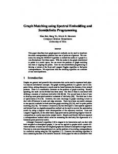
3.1 Validating Manifold Alignment Our framework provides an innovative visualization of temporal social networks as Figure 3 illustrates. Each vertex can be viewed as a trajectory along time axis, while each layer represents the graph embedding in each year. Three important observations can be made from Figure 3: 1. Of all trajectories evolving with time, those without manifold alignment have high temporal variance with large fluctuations; 2. All three alignments have reduced the trajectory variance with different levels; 3. Procrustes alignment performs the best both in magnitude and fluctuation of variance.
1
http://dblp.uni-trier.de/
Figure 3. Trajectories of four different alignments for the real-world DBLP data set with 2,538 core authors: No alignment; Alignment to previous year recursively; Aligned to the 1st year; Procrustes alignment to the 1st year. In all panels, each horizontal layer demonstrates the 2D graph embedding of each year. Each corresponding vertex (author) is linked by line segments going upward. As arrows pointed out in the 1st panel, without alignment, the trajectories have huge variance and fluctuate dramatically. All 3 alignments have reduced the trajectory variance with different levels, among which the Procrustes perform the best.
Figure 4. Gravitational collapse of trajectories to singularity. Left panel: trajectories after manifold alignment for the real-world DBLP data set with 2,538 core authors. Right panel: the conceptual idea of all trajectories converges to singularity (complete graph). Refer to Figure 2 for details. The collapsing phenomenon can be visually inspected, which indicates the diameters of the graphs are shrinking.
3.2 Gravitational collapse of trajectories
3.3 Trajectory Modeling Results
Another interesting phenomenon observed from Figures 3 and 4 (which is not accounted for by previous methods), is that of gravitational collapse of trajectories.
Both linear and quadratic regressions are applied for the estimation and prediction of the author coordinates in year 2004. We fit the model with the first two primary MDS dimensions. For each type of aligned data, the linear fitting has better AIC and BIC scores. Table 1 summarizes the means and the standard deviations of the learning errors for the four types of alignment algorithms. The Procrustes Alignment yields the smallest mean weighed error. It is not surprised that the data without any alignment has errors significantly larger than those from alignment.
In the current formulation of the link prediction problem, the dynamic graph has a fixed vertex set. The edge set increases in time as edges are never deleted (for the DBLP example, this means that if two authors have been linked, they remain linked). It then follows that the diameters of successive graphs (successive network snapshots) are eventually decreasing as the number of shortest paths increases. The graph embedding and the trajectories of each vertex reflect this property. By analogy to the astronomical gravity effect which attracts the mass and eventually every atom will collapse into a singularity, we call this gravitational collapse of trajectories. In the social networks context this corresponds to the convergence of the graphs representing the network to a complete graph.
Figure 5 presents the scatter plots of ground truth coordinates vs. estimated and predicted coordinates for the network in 2004. Prediction has wider variance than estimation, due to the exclusion of the last year data. Alignment plays a significant role in modeling the dynamic graph. The Procrustes alignment method with linear random effect regression performs well in both estimation and prediction, which strongly supports the claim that under this framework, the nature of dynamic social network is sufficiently captured by a simple model.
Table 1. Estimation and Prediction Errors for the four alignments in linear or quadratic nested random effect models. Alignment Method
Regression
Without manifold alignment Affine transform to previous year Affine transform to the 1st year Procrustes alignment
Estimation Error (6)
Estimation Error, Weighted (7)
Prediction Error (6)
Prediction Error, Weighted (7)
AIC
BIC
Linear
192926.1
192942.2
1.7473(1.0435)
1.2271(0.7722)
2.3604(1.4096)
1.6576(1.0432)
Quadratic
209312.2
209328.1
1.1329(0.6530)
0.8544(1.9637)
2.5351(1.4613)
1.9120(4.3943)
Linear
184649.8
184665.8
0.4283(0.2988)
0.3353(0.5095)
0.5785(0.4036)
0.4529(0.6883)
Quadratic
203406.2
203422.0
0.6214(0.4009)
0.5524(2.2990)
1.3905(0.8972)
1.2361(5.1446)
Linear
161244.7
161260.7
0.4043(0.3362)
0.2767(0.6975)
0.5461(0.4541)
0.3738(0.9423)
Quadratic
183140.3
183156.2
0.4938(0.3750)
0.3702(2.0993)
1.1051(0.8392)
0.8283(4.6977)
Linear
162879.5
162895.6
0.4071(0.3324)
0.2716(0.6748)
0.5500(0.4491)
0.3669(0.9116)
Quadratic
184128.5
184144.3
0.5073(0.3750)
0.3677(1.7034)
1.1352(0.8390)
0.8227(3.8117)
Figure 5. The scatter plots of the estimated and predicted coordinates vs. the true coordinates for the DBLP data in 2004. Top: Estimations of the core author coordinates in 2004 using the whole time series. Bottom: Predictions of the core author coordinates in 2004 using whole time series except 2004. Prediction has wider variance than estimation. Alignment plays a significant role in modeling the dynamic graph, especially Procrustes alignment.
3.4 Vertex Behavior Modeling Another functionality enable by this framework is vertex behavior modeling, by clustering the trajectories as shown in Figure 6. Using K-means clustering, we compute 10 clusters which grouped authors with similar temporal behaviors together. Similar trajectories indicate the coevolution patterns of authors. To get more insights into the clustering, Figure 7 takes a closer look into seven authors’ trajectories with highest vertex degrees. Interestingly, five of them have similar trajectories, and they turn out to be all from Israel, compared to the rest two are from different institutes.
3.5 Reconstructing the Predicted Network To reconstruct the predicted network we take the following steps: 4. Predict the graph embedding for the last time point; 5. Collect those pairs of vertices which are not connected by an edge in the graph at the preceding time; 6. Sort the vertices collected at the previous step by their distance: pairs of vertices that are closest in Euclidean space could be potential edges; 7. Prioritize links based on the distances computed above. The reconstruction results are compared against a set of edges created randomly as shown in Table 2. The results of each embedding method with regression methods are reported in terms of how much better they are than a random guess. The percentage of a correct random guess of an edge existence is 0.013%. The consistent superiority of
Figure 7. Trajectory behavior analysis. 7 authors’ trajectories with highest vertex degrees are inspected. Interestingly, YM, NA, DP, MN, MS are all from Israel, and HGM, HER are from different institutes. We observe that these 5 Israeli authors have similar patterns than the rest.
our framework compared random guess suggests that the trend of graph evolution is meaningfully captured. Lastly, the Procrustes alignment method along with a linear regression method proved to be the best performing predictors, which is consistent with Section 3.4.
4. CONCLUSIONS AND FUTURE WORK We have innovatively formulated the problem of link prediction in a network which evolves over time. We
Figure 6. Trajectory behavior clustering for the Procrustes alignment. First row illustrates 10 K-means clusters of temporal trajectory behaviors for DBLP core authors for the 1st MDS dimension. Second row is for the 2nd MDS dimension. The cluster center is superimposed on each plot.
Table 2. Performance of the algorithm with different alignment and regression methods compared to random Without manifold alignment Linear Quadratic Factor of improvement over random
4.49
3.91
Affine transform to previous year Linear Quadratic 4.57
3.93
Affine transform to the 1st year Linear Quadratic 4.78
3.68
Procrustes alignment Linear Quadratic 4.81
3.76
started from the premise that evolution in time of the network requires a dynamic approach, which take into account this evolution (as opposed to approaches based on node similarities in a static, snap shot of the network). This leads us to consider time series approach. However, the challenge for this approach was to extract suitable, useful network characteristics. This was done by embedding the graphs underlying the network (at each time moment) into a continuous space, resulting in a nonlinear subspace or manifold. Essentially for this approach, ensuring reliable prediction and estimation is the step of manifold alignment. Experimental results support this approach both in (i) the need of the alignment, and (ii) estimation and prediction reliability. This proposed framework identifies key components in constructing a good link prediction model, but has not been thoroughly exploited all its potentials. What combinations of these key components will theoretically guarantee a good link prediction result? Is there a theoretical upper or lower bound for link prediction upon this framework? These question remains as future work.
5. ACKNOWLEDGMENTS We appreciate the reviewers’ precious comments.
6. REFERENCES [1] David Liben-Nowell, Jon Kleinber, The link-prediction problem for social networks, Journal of the American Society for Information Science and Technology, Volume 58, Issue 7, pages 1019–1031, May 2007. [2] Lise Getoor, Christopher P. Diehl, Link Mining: A Survey, SIGKDD Explorations, Volume 7, Issue 2
[3] E. Richard, N. Baskiotis, T. Evgeniou, N. Vayatis, Link Discovery using Graph Feature Tracking, NIPS 2010, Vancouver, Canada, December, 2010. [4] Kunegis and Andreas Lommatzsch. 2009. Learning spectral graph transformations for link prediction. In Proceedings of the 26th Annual International Conference on Machine Learning (ICML '09). [5] Kunegis, Damien Fay, and Christian Bauckhage. 2010. Network growth and the spectral evolution model. In Proceedings of the 19th ACM international conference on Information and knowledge management (CIKM '10). [6] Chunsheng Fang, Jason Lu, Anca Ralescu, "Graph Spectra Regression with Low-Rank Approximation for Dynamic Graph Link Prediction", NIPS2010 Workshop on Low-rank Methods for Large-scale Machine Learning, Vancouver, Canada, December, 2010. [7] Nalini Ravishanker, Dipak Dey , A first course in linear model theory, Chapman and Hall/CRC, 2002. [8] Chang Wang and Sridhar Mahadevan. 2008. Manifold alignment using Procrustes analysis. In Proceedings of the 25th international conference on Machine learning (ICML '08). [9] S.V. N. Vishwanathan , et al, Graph Kernels, Journal of Machine Learning Research 2008. [10] Mikhail Belkin, Partha Niyogi , Laplacian Eigenmaps for Dimensionality Reduction and Data Representation, Neural Computation, 2003. [11] J. B. Tenenbaum, V. de Silva and J. C. Langford , A Global Geometric Framework for Nonlinear Dimensionality Reduction, Science, 2000. [12] Young. F. W. and Hamer. R. M. (1994). Theory and Applications of Multidimensional Scaling. Eribaum Associates. Hillsdale, NJ. [13] Chunsheng Fang, Mojtaba Kohram, Anca Ralescu, Towards a Spectral Regression with Low-Rank Approximation Approach for Link Prediction in Dynamic Graphs, IEEE Intelligent Systems Magazine (To appear, July 2011).