MILE: A Multi-Level Framework for Scalable Graph Embedding

MILE: A Multi-Level Framework for Scalable Graph Embedding Jiongqian Liang

The Ohio State University Columbus, Ohio [email protected]

Saket Gurukar

The Ohio State University Columbus, Ohio [email protected]

arXiv:1802.09612v1 [cs.AI] 26 Feb 2018

ABSTRACT Recently there has been a surge of interest in designing graph embedding methods. Few, if any, can scale to a large-sized graph with millions of nodes due to both computational complexity and memory requirements. In this paper, we relax this limitation by introducing the MultI-Level Embedding (MILE) framework – a generic methodology allowing contemporary graph embedding methods to scale to large graphs. MILE repeatedly coarsens the graph into smaller ones using a hybrid matching technique to maintain the backbone structure of the graph. It then applies existing embedding methods on the coarsest graph and refines the embeddings to the original graph through a novel graph convolution neural network that it learns. The proposed MILE framework is agnostic to the underlying graph embedding techniques and can be applied to many existing graph embedding methods without modifying them. We employ our framework on several popular graph embedding techniques and conduct embedding for real-world graphs. Experimental results on five large-scale datasets demonstrate that MILE significantly boosts the speed (order of magnitude) of graph embedding while also often generating embeddings of better quality for the task of node classification. MILE can comfortably scale to a graph with 9 million nodes and 40 million edges, on which existing methods run out of memory or take too long to compute on a modern workstation. ACM Reference Format: Jiongqian Liang, Saket Gurukar, and Srinivasan Parthasarathy. 2018. MILE: A Multi-Level Framework for Scalable Graph Embedding. In Proceedings of ACM conference (Conference’18). ACM, New York, NY, USA, 11 pages. https://doi.org/xxx

1

INTRODUCTION

In recent years, graph embedding has attracted much interest due to its broad applicability for tasks such as vertex classification [20] and full network visualization [24]. However, such methods rarely scale to large datasets (e.g., graphs with over 1 million nodes) since they are computationally expensive and often memory intensive. For example, randomwalk-based embedding techniques, such as DeepWalk [20] and Permission to make digital or hard copies of part or all of this work for personal or classroom use is granted without fee provided that copies are not made or distributed for profit or commercial advantage and that copies bear this notice and the full citation on the first page. Copyrights for third-party components of this work must be honored. For all other uses, contact the owner/author(s). Conference’18, Jan 2018, DC, Washington USA © 2018 Copyright held by the owner/author(s). ACM ISBN 978-x-xxxx-xxxx-x/YY/MM. https://doi.org/xxx

Srinivasan Parthasarathy The Ohio State University Columbus, Ohio [email protected]

Node2Vec [9], require a large amount of CPU time to generate a sufficient number of walks and train the embedding model. As another example, embedding methods based on matrix factorization, including GraRep [3] and NetMF [21], requires constructing an enormous objective matrix (usually much denser than adjacency matrix) on which matrix factorization is performed. Even a medium-size graph with 100K nodes can easily require hundreds of GB of memory using those methods. On the other hand, many graph datasets in the real world tend to be large-scale with millions or even billions of nodes. For instance, Google knowledge graph covers over 570M entities while Facebook friendship graph contains at least 1.39B user dataset with over 1 trillion connections [6]. To the best of our knowledge, none of the existing efforts examines how to scale up graph embedding in a generic way. We make the first attempt to close this gap. We are also interested in the related question of whether the quality of such embeddings can be improved along the way. Specifically, we ask: (1) Can we scale up the existing embedding techniques in an agnostic manner so that they can be directly applied to larger datasets? (2) Can the quality of such embedding methods be strengthened by incorporating the holistic view of the graph? To tackle these problems, we propose a MultI-Level Embedding (MILE) framework for graph embedding. Our approach relies on a three-step process: first, we repeatedly coarsen the original graph into smaller ones by employing a hybrid matching strategy; second, we compute the embeddings on the coarsest graph using an existing embedding mechanism note that graph embedding on the coarsest graph is inexpensive to compute and utilizes far less memory, and moreover intuitively can capture the global structure of the original graph [14, 23]; and third, we propose a novel refinement model based on learning a graph convolution network to refine the embeddings from the coarsest graph to the original graph – learning a graph convolution network allows us to compute a refinement procedure that levers the dependencies inherent to the graph structure and the embedding method of choice. To train this model for embeddings refinement, we design a particular learning task on the coarsest graph, which is efficient to perform. To summarize, we find that: 1) MILE is generalizable. Our MILE framework is agnostic to the underlying graph embedding techniques and treats them as black boxes. We report results on DeepWalk[20], Node2Vec[9], GraRep[3], and NetMF[21]. 2) MILE is scalable. We show that the proposed framework can significantly improve the scalability of the embedding

Conference’18, Jan 2018, DC, Washington USA

Jiongqian Liang, Saket Gurukar, and Srinivasan Parthasarathy

methods (up to 30-fold), by reducing the running time and the memory consumption. 3) MILE generates high-quality embeddings. In many cases, we find that the quality of embeddings improves by levering MILE (in some cases is in excess of 10%). 4) MILE’s ability to learn a data- and embedding- sensitive refinement procedure is key to its effectiveness. Other design choices such as the hybrid coarsening strategy also enable MILE to produce quality embeddings in a scalable fashion.

2

Input graph 𝒢$ Final Embedding ℰ$

𝒢%

𝒢"

Coarsening

Refining

Base Embedding ℰ"

RELATED WORK

Graph Embedding: Many techniques for graph or network embedding have been proposed in recent years. DeepWalk and Node2Vec generate truncated random walks on graphs and apply the Skip Gram by treating the walks as sentences [9, 20]. LINE learns the node embeddings by preserving the firstorder and second-order proximities [24]. Following LINE, SDNE leverages deep neural networks to capture the highly non-linear structure [25]. Other methods construct a particular objective matrix and use matrix factorization techniques to generate embeddings, e.g., GraRep [3] and NetMF [21]. This also led to the proliferation of network embedding methods for information-rich graphs, including heterogeneous information networks [4, 8] and attributed graphs [15, 17, 19, 26]. On the other hand, there are very few efforts, focusing on the scalability of network embedding [1, 13, 27]. Such efforts are specific to a particular embedding strategy and do not offer a generic strategy to scale other embedding techniques. Yet, they still cannot scale to very large graphs. Incidentally, these efforts at scalability are actually orthogonal to our strategy and can potentially be employed along with our efforts to afford even greater speedup. Tangentially related to our work are the recent efforts that develop embedding strategies on multi-layered networks [16, 18]. Distinct from our effort, the networks they studied contain multiple layers in nature with a hierarchical structure. The closest work to this paper is the very recently proposed HARP [5], which proposes a hierarchical paradigm for graph embedding based on iterative learning methods (e.g., DeepWalk and Node2Vec). However, HARP focuses on improving the quality of embeddings by using the learned embeddings from the previous level as the initialized embeddings for the next level, which introduces a huge computational overhead. Moreover, HARP cannot be easily extended to other graph embedding techniques (e.g., GraRep and NetMF) since it needs to modify the embedding methods to preset their initialized embeddings. In this paper, we focus on designing a general purpose framework to scale up embedding methods treating them as black boxes. Multi-level Community Detection: The multi-level approach has been widely studied for efficient community detection [2, 7, 14, 22, 23]. The key idea of these multi-level algorithms is to coarsen the original graph into a much smaller one, which is then partitioned into clusters. The partitions are then recovered from the coarse-grained graph to the original graph in a recursive manner. While our framework shares

ℰ%

Figure 1: An overview of the multi-level embedding framework. some ideas at a conceptual level with such efforts, the objectives are distinct in that we focus on graph embeddings while these methods work on graph partitioning and community discovery.

3

PROBLEM FORMULATION

Let 𝒢 = (𝑉, 𝐸) be the input graph (weighted or unweighted), where 𝑉 and 𝐸 are respectively the node set and edge set. Let 𝐴 be the |𝑉 | × |𝑉 | adjacency matrix of the graph with each entry 𝐴(𝑢, 𝑣) denoting the weight of the edge between node 𝑢 and 𝑣. Without ambiguity, we refer to the graph as 𝒢 and 𝐴 interchangeably in the rest of the paper. We also assume 𝒢 is undirected, though our problem can be easily extended to directed graph. We first define graph embedding: Definition 3.1. Graph Embedding Given a graph 𝒢 = (𝑉, 𝐸) and a pre-defined dimensionality 𝑑 (𝑑 ≪ |𝑉 |), the problem of graph embedding is to learn a 𝑑-dimension vector representation for each node in graph 𝒢 so that graph properties are best preserved. Following this, a graph embedding method is essentially a mapping function 𝑓 : R|𝑉 |×|𝑉 | ↦→ R|𝑉 |×𝑑 , whose input is the adjacency matrix 𝐴 (or 𝒢) and output is a lower dimension matrix. Motivated by the fact that the majority of graph embedding methods cannot scale to large datasets, we seek to speed up existing graph embedding methods without sacrificing quality. We formulate the problem as: Given a graph 𝒢 = (𝑉, 𝐸) and a graph embedding method 𝑓 (·), we aim to realize a strengthened graph embedding method 𝑓^(·) so that it is more scalable than 𝑓 (·) while generating embeddings of comparable or even better quality. We refer to the process of applying 𝑓 (·) on a graph as base embedding, where 𝑓 (·) is called the base embedding method.

4

METHODOLOGY

To address the aforementioned problem, we propose a scalable MultI-Level Embedding (MILE) framework. Our framework is similar to Metis, MLR-MCL, and Graculus [7, 14, 23], which are popular multi-level graph clustering algorithm. Figure 1 shows the overview of our MILE framework, which contains three key phases: graph coarsening, base embedding, and embeddings refining. On the whole, we reduce the size of the graph through repeated coarsening and run graph

MILE: A Multi-Level Framework for Scalable Graph Embedding

D

E

DE

1

2

DE

Conference’18, Jan 2018, DC, Washington USA

A

DE

B

C

D

E

A

BC DE A

2

1

SEM

A 1

1

A

Normalization

A

1

1

1

3∗ 2

3∗ 2 1

B

1

C

B

1

B

C

2∗ 2

NHEM

C

(a) Using SEM and NHEM for graph coarsening

Figure 2: Toy example for illustrating graph

C

A

1 3∗ 2

B

2

D E

2

BC

2

0 2 ' 𝐴" = 𝑀%," 𝐴%𝑀%," = 2 2 2 0

2 0 0

(b) Adjacency matrix and matching matrix

coarsening1 .

(a) shows the process of applying Structural Equivalence Matching (SEM) and Normalized Heavy Edge Matching (NHEM) for graph coarsening. (b) presents the adjacency matrix 𝐴0 of the input graph, the matching matrix 𝑀0,1 corresponding to the SEM and NHEM matchings, and the derivation of the adjacency matrix 𝐴1 of the coarsened graph using Eq. 2. Symbol

Definition

𝒢𝑖 𝑉𝑖 , 𝐸𝑖 𝐴𝑖 , 𝐷𝑖 𝑑 𝑚 𝑓 (·) ℰ𝑖 𝑀𝑖,𝑖+1 ℛ(·) 𝑙

the graph after 𝑖 iterations of coarsening vertex set, edge set of 𝒢𝑖 the adjacency and degree matrix of 𝒢𝑖 dimensionality of the embeddings the total number of coarsening levels the base embedding method applicable on 𝒢𝑖 the embeddings of nodes in 𝒢𝑖 the matching matrix from 𝒢𝑖 to 𝒢𝑖+1 the embeddings refinement model # layers in the graph convolution network

Table 1: Table of notations embedding on the coarsest graph, after which we perform embeddings refinement to recover the embeddings on the original graph. We summarize some important notations in Table 1 and describe our framework in detail below.

4.1

Graph Coarsening

In this phase, the input graph 𝒢 (or 𝒢0 ) is repeatedly coarsened into a series smaller graphs 𝒢1 , 𝒢2 , ..., 𝒢𝑚 such that |𝑉0 | > |𝑉1 | > ... > |𝑉𝑚 |. In order to coarsen a graph from 𝒢𝑖 to 𝒢𝑖+1 , multiple nodes in 𝒢𝑖 are collapsed to form supernodes in 𝒢𝑖+1 , and the edges incident on a super-node are the union of the edges on the original nodes in 𝒢𝑖 [14]. Here the set of nodes forming a super-node is called a matching. The key part of this step is to design a matching approach that can efficiently coarsen the graph while retaining the global structure. In this paper, we propose a hybrid matching technique containing two matching strategies. 4.1.1 Structural Equivalence Matching (SEM). Given two vertices 𝑢 and 𝑣 in an unweighted graph 𝒢, we call they are structurally equivalent if they are incident on the same set of neighborhoods. Theorem 1. If two vertices 𝑢 and 𝑣 in an unweighted graph 𝒢 are structurally equivalent, then their node embeddings derived from 𝒢 will be identical. 1 We follow the strategy in existing work [23] for weighting self-loops (the weight of the self-loop on node 𝐵𝐶 is 2 instead of 1).

This can be proved by reasoning on the fact that the two nodes are non-distinguishable and interchangeable on 𝒢 if they share the same set of the neighborhoods (details of proof omitted due to the limit of space). Base on Theorem 1, we define a structural equivalence matching as a set of nodes that are structurally equivalent to each other. For the example in Figure 2a, nodes 𝐷 and 𝐸 are considered a structural equivalent matching. 4.1.2 Normalized Heavy Edge Matching (NHEM). Heavy edge matching is a popular matching method for graph coarsening [14]. For an unmatched node 𝑢 in 𝒢𝑖 , its heavy edge matching is a pair of vertices (𝑢, 𝑣) such that the weight of the edge between 𝑢 and 𝑣 is the largest. In this paper, we propose to normalize the edge weights when applying heavy edge matching using the formula as follows 𝐴𝑖 (𝑢, 𝑣) 𝑊𝑖 (𝑢, 𝑣) = √︀ . 𝐷𝑖 (𝑢, 𝑢) · 𝐷𝑖 (𝑣, 𝑣)

(1)

In Eq. 1, the weight of an edge is normalized by the degree of the two vertices on which the edge is incident. Intuitively, it penalizes the weights of edges connected with high-degree nodes. For the example in Figure 2a, node 𝐵 is equally likely to be matched with node 𝐴 and node 𝐶 without edge weight normalization. With normalization, node 𝐵 will be matched with 𝐶, which is a better matching since 𝐵 is more structurally similar to 𝐶. As we will show in Sec. 4.3, this normalization is tightly connected with the graph convolution kernel. 4.1.3 A Hybrid Matching Method. In this paper, we use a hybrid of two matching methods above for graph coarsening. To construct 𝒢𝑖+1 from 𝒢𝑖 , we first find out all the structural equivalence matching (SEM) ℳ1 , where 𝒢𝑖 is treated as an unweighted graph. This is followed by the searching of the normalized heavy edge matching (NHEM) ℳ2 on 𝒢𝑖 . Nodes in each matching are then collapsed into a super-node in 𝒢𝑖+1 . Note that some nodes might not be matched at all and they will be directly copied to 𝒢𝑖+1 . Figure 2a provides a toy example for illustrating the process.

Conference’18, Jan 2018, DC, Washington USA

Jiongqian Liang, Saket Gurukar, and Srinivasan Parthasarathy

Formally, we build the adjacency matrix 𝐴𝑖+1 of 𝒢𝑖+1 through matrix operations. To this end, we define the matching matrix storing the matching information from graph 𝒢𝑖 to 𝒢𝑖+1 as a binary matrix 𝑀𝑖,𝑖+1 ∈ {0, 1}|𝑉𝑖 |×|𝑉𝑖+1 | . The 𝑟-th row and 𝑐-th column of 𝑀𝑖,𝑖+1 is set to 1 if node 𝑟 in 𝒢𝑖 will be collapsed to super-node 𝑐 in 𝒢𝑖+1 , and is set to 0 if otherwise. Each column of 𝑀𝑖,𝑖+1 represents a matching with the 1s representing the nodes in it. Each unmatched vertex appears as an individual column in 𝑀𝑖,𝑖+1 with merely one entry set to 1. For the toy example in Figure 2, matching matrix 𝑀0,1 of dimension 5 × 3 indicates the mapping information from the original graph to the coarsened graph. In particular, 2nd row and 3rd row means node 𝐵 and node 𝐶 form a matching and are mapped to super-node 𝐵𝐶 in the coarsened graph (similar for 4th and 5th row). Following this formulation, we construct the adjacency matrix of 𝒢𝑖+1 by using 𝑇 𝐴𝑖+1 = 𝑀𝑖,𝑖+1 𝐴𝑖 𝑀𝑖,𝑖+1 . (2)

Algorithm 1 summarizes the steps of graph coarsening. For each iteration of coarsening, SEM is generated followed by NHEM (line 2-9). A key part of NHEM is to visit the vertices following the ascending order of the number of neighbors (line 5). This is important to ensure most vertices can be matched and the graph can be coarsened significantly. The intuition here is vertices with a smaller number of neighbors have limited choice of finding a match and should be given higher priority for matching (otherwise, once their neighbors are matched by others, these vertices cannot be matched). Algorithm 1 Graph Coarsening

Input: A input graph 𝒢0 , and # levels for coarsening 𝑚. Output: Graph 𝒢𝑖 and matching matrix 𝑀𝑖−1,𝑖 , ∀𝑖 ∈ [1, 𝑚]. 1: for 𝑖 = 1...𝑚 do 2: ℳ1 ← all the structural equivalence matching in 𝒢𝑖−1 . 3: Mark vertices in ℳ1 as matched. 4: ℳ2 = ∅. ◁ storing normalized heavy edge matching 5: Sort 𝑉𝑖−1 by the number of neighbors in ascending order. 6: for 𝑣 ∈ 𝑉𝑖−1 do 7: if 𝑣 and 𝑢 are not matched and 𝑢 ∈ Neighbors(𝑣) then 8: (𝑣, 𝑢) ← the normalized heavy edge matching for 𝑣. 9: ℳ2 = ℳ2 ∪ (𝑣, 𝑢), and mark both as matched. 10: Compute matching matrix 𝑀𝑖−1,𝑖 based on ℳ1 and ℳ2 . 11: Derive the adjacency matrix 𝐴𝑖 for 𝒢𝑖 using Eq. 2. 12: Return graph 𝒢𝑖 and matching matrix 𝑀𝑖−1,𝑖 , ∀𝑖 ∈ [1, 𝑚].

input layer is the embeddings ℰ𝑖+1 of the coarsened graph 𝒢𝑖+1 . The projection layer computes the projected embeddings ℰ𝑖𝑝 based on the matching matrix 𝑀𝑖,𝑖+1 using Eq. 4. Following this, the projected embeddings go through 𝑙 graph convolution layers and output the refined embeddings ℰ𝑖 of graph 𝒢𝑖 at the end. Note the model parameters Θ (𝑘) (𝑘 = 1...𝑙) are shared among all the refinement steps (𝒢𝑖+1 to 𝒢𝑖 , where 𝑖 = 𝑚 − 1...0).

In this paper, we use a wide range of popular embedding methods for base embedding, which includes DeepWalk [20], Node2Vec [9], GraRep [3], and NetMF [21].

4.3

Embeddings Refinement

The final phase of MILE is the embeddings refinement phase. Given a series of coarsened graph 𝒢0 , 𝒢1 , 𝒢2 , ..., 𝒢𝑚 , their corresponding matching matrix 𝑀0,1 , 𝑀1,2 , ..., 𝑀𝑚−1,𝑚 , and the node embeddings ℰ𝑚 on 𝒢𝑚 , we seek to develop an approach to derive the node embeddings of 𝒢0 from 𝒢𝑚 . To this end, we first study an easier subtask: given a graph 𝒢𝑖 , its coarsened graph 𝒢𝑖+1 , the matching matrix 𝑀𝑖,𝑖+1 and the node embeddings ℰ𝑖+1 on 𝒢𝑖+1 , how to infer the embeddings ℰ𝑖 on graph 𝒢𝑖 . Once we solved this subtask, we can then iteratively apply the technique on each pair of consecutive graphs from 𝒢𝑚 to 𝒢0 and eventually derive the node embeddings on 𝒢0 . In this work, we propose to use a graph-based neural network model to perform embeddings refinement. 4.3.1 Graph Convolution Network for Embeddings Refinement. Since we know the matching information between the two consecutive graphs 𝒢𝑖 and 𝒢𝑖+1 , we can easily project the node embeddings from the coarse-grained graph 𝒢𝑖+1 to the fine-grained graph 𝒢𝑖 using 𝑝

ℰ𝑖 = 𝑀𝑖,𝑖+1 ℰ𝑖+1

4.2 Base Embedding on Coarsened Graph The size of the graph reduces drastically after each iteration of coarsening, halving the size of the graph in the best case. We coarsen the graph for 𝑚 iterations and apply the graph embedding method 𝑓 (·) on the coarsest graph 𝒢𝑚 . Denoting the embeddings on 𝒢𝑚 as ℰ𝑚 , we have ℰ𝑚 = 𝑓 (𝒢𝑚 ).

Figure 3: Architecture of the embeddings refinement model. The

(3)

Since our framework is agnostic to the adopted graph embedding method, we can use any graph embedding algorithm for base embedding. Therefore, many existing graph embedding methods can be scaled up using this framework.

(4)

In this case, embedding of a super-node is directly copied to 𝑝 its original node(s). We call ℰ𝑖 the projected embeddings from 𝒢𝑖+1 to 𝒢𝑖 , or simply projected embeddings without ambiguity. While this way of simple projection maintain some information of node embeddings, it has obvious limitations that nodes will share the same embeddings if they are matched and collapsed into a super-node during the coarsening phase. This problem will be more serious when the embedding refinement is performed iteratively from 𝒢𝑚 , ..., 𝒢0 . To address this issue, we propose to use a graph convolution network for embedding refinement. Specifically, we design a graph-based

MILE: A Multi-Level Framework for Scalable Graph Embedding neural network model ℰ𝑖 = ℛ(ℰ𝑖 , 𝐴𝑖 ), which derives the embeddings ℰ𝑖 on graph 𝒢𝑖 based on the projected embeddings 𝑝 ℰ𝑖 and the graph adjacency matrix 𝐴𝑖 . 𝑝

Given a graph 𝐺 with adjacency matrix 𝐴 ∈ R|𝑉 |×|𝑉 | , we consider the graph convolution [12] of 𝑑-channel input signals 𝑋 with filters 𝑔 on 𝐺 as (5)

𝑋 *𝐺 𝑔 = 𝑈 𝜃𝑔 𝑈 𝑇 𝑋.

Here, 𝜃𝑔 = diag(𝜃) is parameterized by spectral multipliers 𝜃 ∈ R|𝑉 | in the Fourier domain, 𝑈 is the matrix of eigenvec1 − 12 tors of the normalized graph Laplacian 𝐿 = 𝐼 − 𝐷∑︀ 𝐴𝐷− 2 , where 𝐷 is a diagonal matrix with entries 𝐷(𝑖, 𝑖) = 𝑗 𝐴(𝑖, 𝑗). Since Eq. 5 can be computationally expensive, we use its fast approximate version from [15]: 1

1

˜ − 2 𝐴˜𝐷 ˜ − 2 𝑋Θ 𝑋 *𝐺 𝑔 ≈ 𝐷 (6) ∑︀ 𝑑×𝑑 ˜ 𝑖) = ˜ where 𝐴˜ = 𝐴 + 𝜆𝐷, 𝐷(𝑖, , and 𝑗 𝐴(𝑖, 𝑗), Θ ∈ R 𝜆 ∈ [0, 1] is a hyper-parameter for controlling the weight of self-loop. As this approximate convolution model can be regarded as a layer-wise linear model, we can stack multiple such layers to achieve a model of higher capacity. The 𝑘-th layer of this neural network model is

(︁

1

1

˜ − 2 𝐴˜𝐷 ˜ − 2 𝐻 (𝑘−1) (𝑋, 𝐴)Θ (𝑘) 𝐻 (𝑘) (𝑋, 𝐴) = 𝜎 𝐷

)︁

(7)

where 𝜎(·) is an activation function, Θ (𝑘) is a layer-specific trainable weight matrix, and 𝐻 (0) (𝑋, 𝐴) = 𝑋. In this paper, we define our embedding refinement model as a 𝑙-layer graph convolution model

(︀

)︀

(︀

)︀

ℰ𝑖 = ℛ ℰ𝑖 , 𝐴𝑖 ≡ 𝐻 (𝑙) ℰ𝑖 , 𝐴𝑖 . (8) The architecture of the refinement model is shown in Figure 3. The intuition behind this refinement model is to integrate the structural information of the current graph 𝒢𝑖 𝑝 into the projected embedding ℰ𝑖 by repeatedly performing the spectral graph convolution. To some extent, each layer of graph convolution network in Eq. 7 can be regarded as one iteration of embedding propagation in the graph following the ˜ − 12 𝐴˜𝐷 ˜ − 12 . Note that this re-normalized adjacency matrix 𝐷 re-normalized matrix is well aligned with the way we conduct normalized heavy edge matching in Eq. 1, where we apply the same way of re-normalization on the adjacency matrix for edge matching. However, we point out that the graph convolution model goes beyond just simple propagation in that the activation function is applied for each iteration of propagation and each dimension of the embedding interacts with other dimensions controlled by the weight matrix Θ (𝑘) . We next discuss how the weight matrix Θ (𝑘) is learned. 𝑝

𝑝

4.3.2 Refinement Model Learning. The learning of the refinement model is essentially learning Θ (𝑘) for each 𝑘 ∈ [1, 𝑙] according to Eq. 7. Here we study how to design the learning task and construct the loss function. Since the graph convolution model 𝐻 (𝑙) (·) aims to predict the embeddings ℰ𝑖 on graph 𝒢𝑖 , we can directly run a base embedding on 𝒢𝑖 to generate the “ground-truth” embeddings and use the difference between these embeddings and the

Conference’18, Jan 2018, DC, Washington USA predicted ones as the loss function for training. We propose to learn Θ (𝑘) on the coarsest graph and reuse them across all the levels for refinement. Specifically, given the coarsest graph 𝒢𝑚 , we first perform base embedding to get ℰ𝑚 = 𝑓 (𝒢𝑚 ), which serves as the “ground truth” for embeddings refinement. We then further coarsen graph 𝒢𝑚 into graph 𝒢𝑚+1 and perform another base embedding: ℰ𝑚+1 = 𝑓 (𝒢𝑚+1 ). Following the embedding refinement procedures, we can predict the refined em𝑝 beddings on 𝒢𝑚 as ℛ(ℰ𝑚 , 𝐴𝑚 ) = 𝐻 (𝑙) (𝑀𝑚,𝑚+1 ℰ𝑚+1 , 𝐴𝑚 ). Considering the “ground truth” from base embedding and inferred embeddings from the refinement model, we can define the loss function as the mean square error as follows 𝐿=

⃦

⃦

1 ⃦ ⃦2 (𝑙) ⃦ℰ𝑚 − 𝐻 (𝑀𝑚,𝑚+1 ℰ𝑚+1 , 𝐴𝑚 ) ⃦ . |𝑉𝑚 |

(9)

We refer to the learning task associated with the above loss function as double-base embedding learning since it requires conducting two times of base embedding in the consecutive layers. We point out, however, there are two key drawbacks to this method. First of all, the above loss function requires one more level of coarsening to construct 𝒢𝑚+1 and an extra base embedding on 𝒢𝑚+1 . These two steps, especially the latter, introduce non-negligible overheads to the MILE framework, which contradicts our motivation of scaling up graph embedding. More importantly, ℰ𝑚 might not be a desirable “ground truth” for the refined embeddings, which are predicted based on ℰ𝑚+1 . This is because most of the embedding methods are invariant to an orthogonal transformation of the embeddings, i.e., the embeddings can be rotated by an arbitrary orthogonal matrix [10]. In other words, the embedding spaces of graph 𝒢𝑚 and 𝒢𝑚+1 can be totally different since the two base embeddings are learned independently. Even if we follow the paradigm in [5] and conduct base embedding on 𝒢𝑚 using 𝑝 the simple projected embeddings from 𝒢𝑚+1 (ℰ𝑚 ) as initialization, the embedding space does not naturally generalize and can drift during re-training. One possible solution is to use an alignment procedure to force the embeddings to be aligned between the two graphs [11]. But it could be very computationally expensive. In this paper, we propose a very simple method to address the above issues. Instead of conducting an additional level of coarsening, we construct a dummy coarsened graph by simply copying 𝒢𝑚 , i.e., 𝑀𝑚,𝑚+1 = 𝐼 and 𝒢𝑚+1 = 𝒢𝑚 . By doing this, we not only reduce one iteration of graph coarsening, but also avoid performing base embedding on 𝒢𝑚+1 simply because ℰ𝑚+1 = ℰ𝑚 . Moreover, the embeddings of 𝒢𝑚 and 𝒢𝑚+1 are guaranteed to be in the same space in this case without any drift. With this strategy, we change the loss function for model learning as follows 𝐿=

⃦

⃦

1 ⃦ ⃦2 (𝑙) ⃦ℰ𝑚 − 𝐻 (ℰ𝑚 , 𝐴𝑚 ) ⃦ . |𝑉𝑚 |

(10)

With the above loss function, we adopt gradient descent with back-propagation to learn the parameters Θ (𝑘) , 𝑘 ∈ [1, 𝑙]. In the subsequent refinement steps, we apply the same set of parameters Θ (𝑘) to infer the refined embeddings. We point out that the training of the refinement model is rather efficient

Conference’18, Jan 2018, DC, Washington USA

Jiongqian Liang, Saket Gurukar, and Srinivasan Parthasarathy

as it is done on the coarsest graph, which is usually much smaller than the original graph. The embeddings refinement process involves merely sparse matrix multiplications using Eq. 8 and is relatively affordable compared to conducting embedding on the original graph. With these different components, we summarize the whole algorithm of our MILE framework in Algorithm 2.

treating the walks as sentences. Following the original work [20], we set the length of random walks as 80, number of walks per node as 10, and context windows size as 10. ∙ Node2Vec (NV) [9]: This is an improved version of DeepWalk, where it generates random walks with more flexibility controlled through parameters 𝑝 and 𝑞. We use the same setting as DeepWalk for those common hyper-parameters while setting 𝑝 = 4.0 and 𝑞 = 1.0, which we found empirically to generate better results across all the datasets. ∙ GraRep (GR) [3]: This method considers different powers (up to 𝑘) of the adjacency matrix to preserve higher-order graph proximity for graph embedding. It uses SVD decomposition to generate the low-dimensional representation of nodes. We set 𝑘 = 4 as suggested in the original work. ∙ NetMF (NM) [21]: It is a recent effort that supports graph embedding via matrix factorization. We set the window size to 10 and the rank ℎ to 1024, and lever the approximate version, as suggested and reported by the authors.

Algorithm 2 Multi-Level Algorithm for Graph Embedding Input: A input graph 𝒢0 = (𝑉0 , 𝐸0 ), # coarsening levels 𝑚, and a base embedding method 𝑓 (·). Output: Graph embeddings ℰ0 on 𝒢0 .

Use Algorithm 1 to coarsen 𝒢0 into 𝒢1 , 𝒢2 , ..., 𝒢𝑚 . Perform base embedding on the coarsest graph 𝒢𝑚 (See Eq. 3). Learn the weights Θ (𝑘) using the loss function in Eq. 10. for 𝑖 = (𝑚 − 1)...0 do Compute the projected embeddings ℰ𝑖𝑝 on 𝒢𝑖 using Eq. 4. Use Eq. 7 and Eq. 8 to compute refined embeddings ℰ𝑖 . 7: Return graph embeddings ℰ0 on 𝒢0 .

1: 2: 3: 4: 5: 6:

5

EXPERIMENTS AND ANALYSIS

In this section, we conduct extensive experiments to gain more insights on the proposed MILE framework. Dataset PPI Blog Flickr YouTube Yelp

# Nodes 3,852 10,312 80,513 1,134,890 8,938,630

# Edges 37,841 333,983 5,899,882 2,987,624 39,821,123

# Classes 50 39 195 47 22

Table 2: Dataset Information

5.1

Experimental Configuration

Datasets: The datasets used in our experiments is shown in Table 2 and are detailed below: ∙ PPI is a Protein-Protein Interaction graph constructed based on the interplay activity between proteins of Homo Sapiens, where the labels represent biological states. ∙ Blog is a network of social relationship of bloggers on BlogCatalog and the labels indicate interests of the bloggers. ∙ Flickr is a social network of the contacts between users on flickr.com with labels denoting the interest groups. ∙ YouTube is a social network between users on YouTube, where labels represent genres of groups subscribed by users. ∙ Yelp is a social network of friends on Yelp and labels indicate the business categories on which the users review. The first four datasets have been previously used to evaluate graph embedding strategies [9, 20, 21], while Yelp is a dataset preprocessed by us following similar procedures in [13]2 . Baseline Methods: To demonstrate that MILE can work with different graph embedding methods, we explore several popular methods for graph embedding. ∙ DeepWalk (DW) [20]: This method generates truncated random walks on graphs and applies the Skip Gram by 2

Raw data: https://www.yelp.com/dataset_challenge/dataset

MILE-specific Settings: When applying our MILE framework, we vary the coarsening levels 𝑚 from 1 to 10 whenever possible. For the graph convolution network model, the self-loop weight 𝜆 is set to 0.05, the number of hidden layers 𝑙 is 2, and tanh(·) is used as the activation function, the learning rate is set to 0.001 and the number of training epochs is 200. The Adam Optimizer is used for model training. System Specification: The experiments were conducted on a machine running Linux with an Intel Xeon E5-2680 CPU (28 cores, 2.40GHz) and 128 GB of RAM. For all the four base embedding methods, we adapt the original code from the authors3 . We additionally use TensorFlow package for the embeddings refinement learning component. We lever the available parallelism (on 28 cores) for each method (e.g., the generation of random walks in DeepWalk and Node2Vec, the training of the refinement model in MILE, etc.). Evaluation Metrics: To evaluate the quality of the embeddings, we follow the typical method in existing work to perform multi-label node classification [9, 20]. Specifically, after the graph embeddings are learned for nodes (label is not used for this part), we run a 10-fold cross validation using the embeddings as features and report the average Micro-F1 and average Macro-F1. We also record the end-to-end wallclock time consumed by each method for scalability comparisons.

5.2

MILE Framework Performance

We first evaluate the performance of our MILE framework when applied to different graph embedding methods. For each dataset, we show the results of MILE under two settings of coarsening levels 𝑚 and expand on the remaining results in the next section. Table 3 summarizes the performance of MILE on different datasets with various base embedding methods4 . We make the following observations: 3 DeepWalk: https://github.com/phanein/deepwalk; Node2Vec: https://github.com/aditya-grover/node2vec; GraRep: https://github. com/thunlp/OpenNE; NetMF: https://github.com/xptree/NetMF 4 We discuss the results of Yelp later.

MILE: A Multi-Level Framework for Scalable Graph Embedding Method DeepWalk MILE (DW, 𝑚 = 1) MILE (DW, 𝑚 = 2) Node2Vec MILE (NV, 𝑚 = 1) MILE (NV, 𝑚 = 2) GraRep MILE (GR, 𝑚 = 1) MILE (GR, 𝑚 = 2) NetMF MILE (NM, 𝑚 = 1) MILE (NM, 𝑚 = 2)

Micro-F1 23.0 25.6(11.3%↑) 25.5(10.9%↑) 24.3 25.9(6.6%↑) 26.0(7.0%↑) 25.5 25.6(0.4%↑) 25.3(-0.8%↓) 24.6 26.9(9.3%↑) 26.7(8.5%↑)

Macro-F1 18.6 20.4(9.7%↑) 20.7(11.3%↑) 19.6 20.6(5.1%↑) 21.1(7.7%↑) 20.0 19.8(-1.0%↓) 19.5(-2.5%↓) 20.1 21.6(7.5%↑) 21.1(5.0%↑)

Time (mins) 2.42 1.22(2.0×) 0.67(3.6×) 4.01 1.77(2.3×) 0.98(4.1×) 2.99 1.11(2.7×) 0.43(6.9×) 0.65 0.27(2.5×) 0.17(3.9×)

Conference’18, Jan 2018, DC, Washington USA Method DeepWalk MILE (DW, 𝑚 = 1) MILE (DW, 𝑚 = 2) Node2Vec MILE (NV, 𝑚 = 1) MILE (NV, 𝑚 = 2) GraRep MILE (GR, 𝑚 = 1) MILE (GR, 𝑚 = 2) NetMF MILE (NM, 𝑚 = 1) MILE (NM, 𝑚 = 2)

Micro-F1 40.0 40.4(1.0%↑) 39.3(-1.8%↓) 40.5 40.7(0.5%↑) 38.8(-4.2%↓) N/A 36.7 36.3 31.8 39.3(23.6%↑) 39.5(24.2%↑)

Macro-F1 26.5 27.3(3.0%↑) 26.1(-1.5%↓) 27.3 27.7(1.5%↑) 25.8(-5.5%↓) N/A 18.6 18.6 14.0 24.5(75.0%↑) 25.9(85.0%↑)

Macro-F1 21.0 27.0(28.6%↑) 23.5(11.9%↑) 23.0 26.4(14.8%↑) 23.9(3.9%↑) 23.3 24.0(3.0%↑) 20.4(-12.4%↓) 25.0 27.6(10.4%↑) 25.5(2.0%↑)

Time (mins) 8.02 4.69(1.7×) 2.71(3.0×) 13.04 6.99(1.9×) 3.89(3.4×) 28.76 12.25(2.3×) 4.22(6.8×) 2.64 1.98(1.3×) 1.27(2.1×)

(b) Blog Dataset

(a) PPI Dataset

Method DeepWalk MILE (DW, 𝑚 = 1) MILE (DW, 𝑚 = 2) Node2Vec MILE (NV, 𝑚 = 1) MILE (NV, 𝑚 = 2) GraRep MILE (GR, 𝑚 = 1) MILE (GR, 𝑚 = 2) NetMF5 MILE (NM, 𝑚 = 1) MILE (NM, 𝑚 = 2)

Micro-F1 37.0 42.9(15.9%↑) 39.4(6.5%↑) 39.1 42.8(9.5%↑) 40.2(2.8%↑) 40.6 41.7(2.7%↑) 38.3(-5.7%↓) 41.4 43.8(5.8%↑) 42.4(2.4%↑)

Time (mins) 50.08 34.48(1.5×) 26.88(1.9×) 78.21 50.54(1.5×) 36.85(2.1×) > 2343.37 697.39(>3.4×) 163.05(>14.4×) 69.72 24.03(2.9×) 15.84(4.4×)

(c) Flickr Dataset

Method DeepWalk MILE (DW, 𝑚 = 6) MILE (DW, 𝑚 = 8) Node2Vec MILE (NV, 𝑚 = 6) MILE (NV, 𝑚 = 8) GraRep MILE (GR, 𝑚 = 6) MILE (GR, 𝑚 = 8) NetMF MILE (NM, 𝑚 = 6) MILE (NM, 𝑚 = 8)

Micro-F1 45.2 46.1(2.0%↑) 44.3(-2.0%↓) 45.5 46.3(1.8%↑) 44.3(-2.6%↓) N/A 43.2 42.3 N/A 40.9 39.2

Macro-F1 34.7 38.5(11.0%↑) 35.3(1.7%↑) 34.6 38.3(10.7%↑) 35.8(3.5%↑) N/A 32.7 30.9 N/A 27.8 25.5

Time (mins) 604.83 55.20(11.0×) 37.35(16.2×) 951.27 83.52(11.4×) 55.55(17.1×) > 3167.00 1644.89(>1.9×) 673.95(>4.7×) > 574.75 35.22(>16.3×) 19.22(>29.9×)

(d) YouTube Dataset

Table 3: Performance of MILE compared to the original embedding methods. DeepWalk, Node2Vec, GraRep, and NetMF denotes the original

method without using our MILE framework. We set the number of coarsening levels 𝑚 to 1 and 2 for PPI, Blog and Flickr, while choosing 6 and 8 for YouTube (due to its larger scale). The Micro-F1 and Macro-F1 are in 10−2 scale while the column Time shows the running time in minutes. The numbers within the parenthesis by the reported Micro-F1 and Macro-F1 scores are the relative percentage of change compared to the original method, e.g., MILE (DW, 𝑚 = 1) vs. DeepWalk. “↑” and “↓” respectively indicate improvement and decline. Numbers along with “×” is the speedup compared to the original method. “N/A” indicates the method runs out of 128 GB memory and we show the amount of running time spent when it happens.

∙ MILE is scalable. MILE greatly boosts the speed of the explored embedding methods. With a single level of coarsening (𝑚=1), we are able to achieve speedup ranging from 1.5× to 3.4× (on PPI, Blog, and Flickr) while improving qualitative performance. Larger speedups are typically observed on GraRep and NETMF. Increasing the coarsening level 𝑚 to 2, the speedup increases further (up to 14.4×), while the quality of the embeddings is comparable with the original methods reflected by Micro-F1 and Macro-F1. On the largest datasets among the four (YouTube) where the coarsening level is 6 and 8, we observe more than 10× speedup for DeepWalk and Node2Vec. For NetMF, the speedup is even larger (more than 16×) – original NetMF runs out of memory within 9.5 hours while MILE (NM) only takes around 35 minutes (𝑚 = 6) or 20 minutes (𝑚 = 8).

5 The NetMF paper [21], reports different results on Flickr with 𝑑 = 128 and rank ℎ = 1024, which we were unable to replicate. In personal communication, its first author promptly acknowledged the error - a much larger rank ℎ is needed to achieve the reported results, which comes at a significant computation and memory cost (their results are on a machine with 1TB of memory).

∙ MILE improves quality. For the smaller coarsening levels across all the datasets and methods, MILE-enhanced embeddings almost always offer a qualitative improvement over the original embedding method as evaluated by the Micro-F1 score and Macro-F1 score (as high as 28.6% while many others also show an 10%+ increase). Evident examples include MILE (DW, 𝑚 = 1) on Blog/PPI and MILE (NM, 𝑚 = 1) on PPI/Blog/Flickr. Even with the higher number of coarsening level (𝑚 = 2 for PPI/Blog/Flickr; 𝑚 = 8 for YouTube), MILE in addition to being much faster can still improve, qualitatively, over the original methods on all datasets, e.g., MILE(NM, 𝑚 = 2) ≫ NETMF on PPI, Blog, and Flickr. We conjecture the observed improvement on quality is because the embeddings begin to rely on a more holistic view of the graph. ∙ MILE supports multiple embedding strategies. We make some embedding-specific observations here. We observe that MILE consistently improves both the quality and the efficiency of NetMF on all four datasets (for YouTube the base method runs out of memory). For the largest dataset the speedups afforded exceed 30-fold. We observe that for GraRep, while speedups with MILE are consistently observed, the qualitative improvements, if any, are smaller

Conference’18, Jan 2018, DC, Washington USA (for both YouTube and Flickr, the base method runs out of memory). For DeepWalk and Node2Vec, we again observe consistent improvements in scalability (up to 11-fold on the largest dataset) as well as quality using MILE with a single level of coarsening (or 𝑚 = 6 for YouTube). However, when the coarsening level is increased, the additional speedup afforded (up to 17-fold) comes at a mixed cost to quality (micro-F1 drops slightly while macro-F1 improves slightly). To summarize, our MILE framework not only significantly speeds up the embedding methods, but also improves the quality of the node embeddings. We do notice that it negatively affects the embeddings in some case when the number of coarsening levels is large, e.g., MILE (GR, 𝑚 = 2) on PPI and Blog. But we point out the decrease is mostly minor compared to large speedup achieved. Moreover, we can reduce the coarsening levels in order to generate better embeddings (e.g., 𝑚 = 1) if the quality of the embeddings is valued over efficiency. We discuss the trade-off between quality and efficiency of graph embedding in Sec. 5.4

5.3 MILE Drilldown: Design Choices We now study the role of the design choices we make within the MILE framework related to the coarsening and refinement procedures described. To this end, we examine alternative design choices and systematically examine their performance. The alternatives we consider are: ∙ Random Matching (MILE-rm): We replace Algorithm 1 with a simple random matching approach for graph coarsening. For each iteration of coarsening, we repeatedly pick a random pair of connected nodes as a match and merge them into a super-node until no more matching can be found. The rest of the algorithm is the same as our MILE. ∙ Simple Projection (MILE-proj): We replace our embedding refinement model with a simple projection method. In other words, we directly copy the embedding of a super-node to its original node(s) without any refinement (see Eq. 4). ∙ Averaging Neighborhoods (MILE-avg): For this baseline method, the refined embedding of each node is a weighted average node embeddings of its neighborhoods (weighted by the edge weights). This can be regarded as an embeddings propagation method. We add self-loop to each node6 and conduct the embeddings propagation for two rounds. ∙ Untrained Refinement Model (MILE-untr): Instead of training the refinement model to minimize the loss defined in Eq. 10, this baseline merely uses a fix set of values for parameters Θ (𝑘) without training (values are randomly generated; other parts of the model in Eq. 7 are the same, ˜ including 𝐴˜ and 𝐷). ∙ Double-base Embedding for Refinement Training (MILE2base): This method replaces the loss function in Eq. 10 with the alternative one in Eq. 9 for model training. It conducts one more layer of coarsening and base embedding (level 𝑚 + 1), from which the embeddings are projected to level 𝑚 and used as the input for model training. 6

Self-loop weights are tuned to the best performance.

Jiongqian Liang, Saket Gurukar, and Srinivasan Parthasarathy

DeepWalk MILE (DW) MILE-rm (DW) MILE-proj (DW) MILE-avg (DW) MILE-untr (DW) MILE-2base (DW) MILE-gs (DW)

PPI Mi-F1 Time 23.0 2.42 25.6 1.22 25.3 1.01 20.9 1.12 23.5 1.07 23.5 1.08 25.4 2.22 22.4 2.03

Blog Mi-F1 Time 37.0 8.02 42.9 4.69 40.4 3.62 34.5 3.92 37.7 3.86 35.5 3.96 35.6 6.74 35.3 6.44

Flickr Mi-F1 Time 40.0 50.08 40.4 34.48 38.9 26.67 35.5 25.99 37.2 25.99 37.6 26.02 37.7 53.32 36.4 44.81

YouTube Mi-F1 Time 45.2 604.83 46.1 55.20 44.9 55.10 40.7 53.97 41.4 55.26 41.8 54.52 41.6 94.74 43.6 394.72

NetMF MILE (NM) MILE-rm (NM) MILE-proj (NM) MILE-avg (NM) MILE-untr (NM) MILE-2base (NM) MILE-gs (NM)

24.6 26.9 25.2 23.5 24.5 24.8 26.6 24.8

41.4 43.8 41.0 38.7 39.9 39.4 41.3 40.0

31.8 39.3 37.6 34.5 36.4 36.4 37.7 35.1

N/A 40.9 39.6 26.4 26.4 30.2 34.7 36.4

0.65 0.27 0.22 0.12 0.13 0.13 0.29 1.08

2.64 1.98 1.69 1.06 1.05 1.08 2.33 3.70

69.72 24.03 20.00 15.10 14.86 15.23 31.65 34.25

>574 35.22 33.52 26.48 27.71 27.20 55.18 345.28

Table 4: Comparisons of graph embeddings between MILE and its

variants. Except for the original methods (DeepWalk and NetMF), the number of coarsening level 𝑚 is set to 1 on PPI/Blog/Flickr and 6 on YouTube. Mi-F1 is the Micro-F1 score in 10−2 scale while Time column shows the running time of the method in minutes. “N/A” denotes the method consumes more than 128 GB RAM.

∙ GraphSAGE as Refinement Model (MILE-gs): It replaces the graph convolution network in our refinement method with GraphSAGE [10]7 . We choose max-pooling for aggregation and set the number of sampled neighbors as 100, as suggested by the authors. Also, concatenation is conducted instead of replacement during the process of propagation. Table 4 shows the comparison of performance on these methods across the four datasets. Due to limit of space, we focus on using DeepWalk and NetMF for base embedding with a smaller coarsening level (𝑚 = 1 for PPI, Blog, and Flickr; 𝑚 = 6 for YouTube). Results are similar for the other embedding options we consider. We hereby summarize the key information derived from Table 4 as follows: ∙ The matching methods used within MILE offer a qualitative benefit at a minimal cost to execution time. Comparing MILE with MILE-rm for all the datasets, we can see that MILE generates better embeddings than MILE-rm using either DeepWalk or NetMF as the base embedding method. Though MILE-rm is slightly faster than MILE due to its random matching, its Micro-F1 score and Macro-F1 score are consistently lower than of MILE. ∙ The graph convolution based refinement learning methodology in MILE is particularly effective. Simple projection based MILE-proj, performs significantly worse than MILE. The other two variants (MILE-avg and MILE-untr) which do not train the refinement model at all, also perform much worse than the proposed method. Note MILE-untr is the same as MILE except it uses a default set of parameters instead of learning those parameters. Clearly, the model learning part of our refinement method is a fundamental contributing factor to the effectiveness of MILE. Through training, the refinement model is tailored to the specific graph under the base embedding method in use. The overhead cost of this learning (comparing MILE with MILE-untr), can vary depending on the base embedding 7

Adapt code from https://github.com/williamleif/GraphSAGE

MILE: A Multi-Level Framework for Scalable Graph Embedding

2 # Levels

3

4

0

1

0

1

2 # Levels

3 4 # Levels

5

6

3

(e) PPI (Running Time)

4

Micro-f1

MILE (NetMF)

0 1 2 3 4 5 6 7 8 # Levels

0.52 0.50 0.48 0.46 0.44 0.42 0.40 0.38

(c) Flickr (Micro-F1)

0 1 2 3 4 5 6 7 8 # Levels (d) YouTube (Micro-F1)

103

101

Time (mins)

100

10

2

(b) Blog (Micro-F1)

Time (mins)

Time (mins)

(a) PPI (Micro-F1)

1

MILE (GraRep)

0.45 0.40 0.35 0.30 0.25 0.20 0.15

100

Time (mins)

1

0.45 0.40 0.35 0.30 0.25 0.20 0.15

MILE (Node2Vec)

Micro-f1

Micro-f1

Micro-f1

MILE (DeepWalk) 0.30 0.28 0.26 0.24 0.22 0.20 0.18 0

Conference’18, Jan 2018, DC, Washington USA

102

102

101 0

1

2

3 4 # Levels

5

6

(f) Blog (Running Time)

0 1 2 3 4 5 6 7 8 # Levels (g) Flickr (Running Time)

0 1 2 3 4 5 6 7 8 # Levels (h) YouTube (Running Time)

Figure 4: Changes in performance as the number of coarsening levels in MILE increases (best viewed in color). Micro-F1 and running-time are

reported in the first and second row respectively. Running time in minutes is shown in logarithm scale. Note that # level = 0 represents the original embedding method without using MILE. Lines/points are missing for algorithms that use over 128 GB of RAM.

employed (for instance on the YouTube dataset, it is an insignificant 1.2% on DeepWalk - while being up to 20% on NetMF) but is still worth it due to qualitative benefits (Micro-F1 up from 30.2 to 40.9 with NetMF on YouTube). ∙ Graph convolution refinement learning outperforms GraphSAGE. Replacing the graph convolution network with GraphSAGE for embeddings refinement, MILE-gs does not perform as well as MILE. It is also computationally more expensive, partially due to its reliance on embeddings concatenation, instead of replacement, during the process the embeddings propagation (higher model complexity). ∙ Double-base embedding learning is not effective. In Sec. 4.3.2, we discuss the issues with unaligned embeddings of the double-base embedding method for the refinement model learning. The performance gap between MILE and MILE2base in Table 4 provides empirical evidence supporting our argument. This gap is likely caused by the fact that the base embeddings of level 𝑚 and level 𝑚 + 1 might not lie in the same embedding space (rotated by some orthogonal matrix) [10]. As a result, using the projected 𝑝 embeddings ℰ𝑚 as input for model training (MILE-2base) is not as good as directly using ℰ𝑚 (MILE). Moreover, Table 4 shows that the additional round of base embedding in MILE-2base introduces a non-trivial overhead. On YouTube, the running time of MILE-2base is 1.6 times as much as MILE.

contains less than 128 nodes (it is trivial to embed such a graph into 128 dimensions). Figure 4 shows the changes of Micro-F1 for node classification and running time of MILE as 𝑚 increases. We underline the following observations:

5.4

We now study the impact of MILE on reducing memory consumption. For this purpose, we focus on MILE (GraRep) and MILE (NetMF), with GraRep and NetMF as base embedding methods respectively. Both of these are embedding

MILE Drilldown: Varying Coarsening Levels

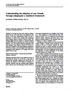
We now study the performance of the MILE framework as we vary the number of coarsening levels 𝑚. Starting from 𝑚 = 0, we increase 𝑚 until it reaches 8 or the coarsest graph

∙ When coarsening level 𝑚 is small, MILE tends to significantly improve the quality of embeddings while taking much less time. From 𝑚 = 0 (i.e., without applying the MILE framework) to 𝑚 = 1, we see a clear jump of the Micro-F1 score on all the datasets across the four base embedding methods. This observation is more evident on larger datasets (Flickr and YouTube). On YouTube, MILE (DeepWalk) with 𝑚=1 increases the Micro-F1 score by 5.3% while only consuming half of time compared to the original DeepWalk. MILE (DeepWalk) continues to generate embeddings of better quality than DeepWalk until 𝑚 = 7, where the speedup is 13×. ∙ As the coarsening level 𝑚 in MILE increases, the running time drops dramatically while the quality of embeddings only decreases slightly. The running time decreases at an almost exponential rate (logarithm scale on the y-axis in the second row of Figure 4). On the other hand, the MicroF1 score descends much more slowly (first row of Figure 4). Sacrificing a tiny fraction of quality on embeddings can save a huge amount of computational resource.

5.5

MILE Drilldown: Memory Consumption

Jiongqian Liang, Saket Gurukar, and Srinivasan Parthasarathy

5.7

1.4

Memory in (GB)

Memory in (GB)

8 6 4 2 0

1.2 1.0 0.8 0.6 0.4 0.2

0

1

2

3

4

Coarsening level

5

6

0.0

(a) MILE (GraRep)

0

1

2

3

4

Coarsening level

5

6

(b) MILE (NetMF)

Figure 5: Memory consumption of MILE (GraRep) and MILE (NetMF) on Blog with varied coarsening levels. Coarsening level 0 corresponds to the original embedding method without applying the MILE framework.

DeepWalk MILE (DW) HARP (DW)

PPI Mi-F1 Time 23.0 2.42 25.6 1.22 24.1 3.08

Blog Mi-F1 Time 37.0 8.02 42.9 4.69 41.3 9.85

Flickr Mi-F1 Time 40.0 50.08 40.4 34.48 40.6 78.21

YouTube Mi-F1 Time 45.2 604.83 46.1 55.20 46.6 1727.78

Table 5: Comparisons of MILE with HARP. methods based on matrix factorization, which possibly involves a dense objective matrix and could be rather memory expensive. We do not explore DeepWalk and Node2Vec here since their embedding learning methods generate truncated random walks (training data) on the fly with almost negligible memory consumption (compared to the space storing the graph and the embeddings). Figure 5 shows the memory consumption of MILE (GraRep) and MILE(NetMF) as the coarsening level increases on Blog (results on other dataset are similar). We observe that MILE significantly reduces the memory consumption as the coarsening level increases. Even with one level of coarsening, the memory consumption of GraRep and NetMF reduces by 64% and 42% respectively. The dramatic reduction continues as the coarsening level increases until it reaches 4, where the memory consumption is mainly contributed by the storage of the graph and the embeddings. This memory reduction is consistent with our intuition, since both # rows and # columns in the objective matrix for factorization reduce almost by half with one level of coarsening.

5.6 Comparing MILE with HARP HARP is a recent multi-level method primarily for improving the quality of graph embeddings. We compare HARP with our MILE framework using DeepWalk as the base embedding method8 . Table 5 shows the performance of these two methods on the four datasets (coarsening level is 1 on PPI/Blog/Flickr and 6 on YouTube). From the table we can observe that MILE generates embeddings of comparable quality with HARP. MILE performs much better than HARP on PPI and Blog but falls slightly behind on Flickr and YouTube. However, MILE is significant faster than HARP on all the four datasets (e.g. on YouTube, MILE affords a 31× speedup). This is because HARP requires running the whole embedding algorithm on each coarsened graph, which introduces a huge computational overhead (see Sec. 2 for more discussions). 8 We use the source code from the authors: https://github.com/ GTmac/HARP. Results on Node2Vec are similar and hence omitted.

MILE: Large Graph Embedding

We now explore the scalability of our MILE framework on the large Yelp dataset. To the best our knowledge, Yelp is one of the largest datasets for a graph embedding task in the literature with around 9 million nodes and 40 million edges. None of the four graph embedding methods studied in this paper can successfully conduct graph embedding on Yelp within 60 hours on a modern machine with 28 cores and 128 GB RAM (two run out of memory). Leveraging the proposed MILE framework, however, makes it possible to perform graph embedding on this scale of datasets. To this end, we run the MILE framework on Yelp using the four graph embedding techniques as the base embedding methods with various coarsening levels (see Figure 6 for the results). We observe that MILE significantly reduces the running time while the Micro-F1 score remains almost unchanged. For example, MILE reduces the running time of DeepWalk from 53 hours (coarsening level 4) to 2 hours (coarsening level 22) while reducing the Micro-F1 score just by 1% (from 0.643 to 0.634). Meanwhile, there is no change in the MicroF1 score from coarsening level 4 to 10, where the running time is improved by a factor of two. These results affirm the power of the proposed MILE framework on scaling up graph embedding algorithms while generating quality embeddings. MILE (DeepWalk)

MILE (Node2Vec)

MILE (GraRep)

MILE (NetMF)

0.70 0.68 Micro-f1

1.6 10

Time (mins)

Conference’18, Jan 2018, DC, Washington USA

0.66 0.64

103

0.62 0.60 0 2 4 6 8 10 12 14 16 18 20 22 # Levels

(a) Micro-F1

102 0 2 4 6 8 10 12 14 16 18 20 22 # Levels

(b) Running Time

Figure 6: Running MILE on Yelp dataset. Lines/points are missing

for algorithms that do not finish within 60 hours or use over 128 GB of RAM.

6

CONCLUSION

In this work, we propose a novel multi-level embedding (MILE) framework to scale up graph embedding techniques, without modifying them. Our framework incorporates existing embedding techniques as black boxes, and significantly improves the scalability of extant methods by reducing both the running time and memory consumption. Additionally, MILE also provides a lift in the quality of node embeddings in most of the cases. A fundamental contribution of MILE is its ability to learn a refinement strategy that depends on both the underlying graph properties and the embedding method in use. In the future, we plan to generalize our framework for information-rich graphs, such as heterogeneous information networks and attributed graphs. Acknowledgments: This work is supported by the National Science Foundation under grants EAR-1520870 and DMS1418265. Computational support was provided by the Ohio Supercomputer Center under grant PAS0166. All content

MILE: A Multi-Level Framework for Scalable Graph Embedding represents the opinion of the authors, which is not necessarily shared or endorsed by their sponsors.

REFERENCES

[1] N. K. Ahmed and et al. A framework for generalizing graph-based representation learning methods. In arXiv’17’. [2] V. D. Blondel and et al. Fast unfolding of communities in large networks. In J. Stat. Mech. Theory Exp. ’08. [3] S. Cao, W. Lu, and Q. Xu. Grarep: Learning graph representations with global structural information. In CIKM’15. [4] S. Chang and et al. Heterogeneous network embedding via deep architectures. In KDD’15. [5] H. Chen, B. Perozzi, Y. Hu, and S. Skiena. Harp: Hierarchical representation learning for networks. In AAAI’18. [6] A. Ching, S. Edunov, M. Kabiljo, D. Logothetis, and S. Muthukrishnan. One trillion edges: Graph processing at facebook-scale. In VLDB’15. [7] I. S. Dhillon, Y. Guan, and B. Kulis. Weighted graph cuts without eigenvectors a multilevel approach. In PAMI’07. [8] Y. Dong, N. V. Chawla, and A. Swami. metapath2vec: Scalable representation learning for heterogeneous networks. In KDD’17. [9] A. Grover and J. Leskovec. node2vec: Scalable feature learning for networks. In KDD’16. [10] W. Hamilton, Z. Ying, and J. Leskovec. Inductive representation learning on large graphs. In NIPS’17. [11] W. L. Hamilton, J. Leskovec, and D. Jurafsky. Diachronic word embeddings reveal statistical laws of semantic change. In ACL’16. [12] M. Henaff, J. Bruna, and Y. LeCun. Deep convolutional networks on graph-structured data. In arXiv’15’. [13] X. Huang, J. Li, and X. Hu. Accelerated attributed network embedding. In SDM’17. [14] G. Karypis and V. Kumar. Multilevelk-way partitioning scheme for irregular graphs. In JPDC’98. [15] T. N. Kipf and M. Welling. Semi-supervised classification with graph convolutional networks. In ICLR’17. [16] J. Li, C. Chen, H. Tong, and H. Liu. Multi-layered network embedding. In SDM’18. [17] J. Liang, P. Jacobs, J. Sun, and S. Parthasarathy. Semi-supervised embedding in attributed networks with outliers. In SDM’18. [18] W. Liu, P.-y. Chen, S. Yeung, T. Suzumura, and L. Chen. Principled multilayer network embedding. In ICDM’17. [19] S. Pan, J. Wu, X. Zhu, C. Zhang, and Y. Wang. Tri-party deep network representation. In IJCAI’16. [20] B. Perozzi, R. Al-Rfou, and S. Skiena. Deepwalk: Online learning of social representations. In KDD’14. [21] J. Qiu, Y. Dong, H. Ma, J. Li, K. Wang, and J. Tang. Network embedding as matrix factorization: Unifyingdeepwalk, line, pte, and node2vec. In WSDM’18. [22] Y. Ruan, D. Fuhry, J. Liang, Y. Wang, and S. Parthasarathy. Community discovery: Simple and scalable approaches. In User Community Discovery. 2015. [23] V. Satuluri and S. Parthasarathy. Scalable graph clustering using stochastic flows: applications to community discovery. In KDD’09. [24] J. Tang, M. Qu, M. Wang, M. Zhang, J. Yan, and Q. Mei. Line: Large-scale information network embedding. In WWW’15. [25] D. Wang, P. Cui, and W. Zhu. Structural deep network embedding. In KDD’2016. [26] C. Yang, Z. Liu, D. Zhao, M. Sun, and E. Y. Chang. Network representation learning with rich text information. In IJCAI’15. [27] C. Yang, M. Sun, Z. Liu, and C. Tu. Fast network embedding enhancement via high order proximity approximation. In IJCAI’17.

Conference’18, Jan 2018, DC, Washington USA