APCOM & ISCM 11-14 December, 2013, Singapore th
Graph grammar based multi-frontal direct solver for isogeometric FEM simulations on GPU *M. Paszyński¹, K. Kuźnik1, V.M. Calo2 and D. Pardo3 1
AGH University of Science and Technology, Krakow, Poland. King Abdullah University of Science and Technology, Thuwal, Saudi Arabia. 3 The University of the Basque Country, UPV/EHU and Ikerbasque, Bilbao, Spain. 2
*Corresponding author:
[email protected]
Abstract We present a multi-frontal direct solver for two dimensional isogeometric finite element method simulations with NVIDIA CUDA and perform numerical experiments for linear, quadratic and cubic B-splines. We compare the computational cost O(Np2) for 2D parallel shared memory implementation with the corresponding estimate O(N1.5p3) for a standard 2D sequential implementation. We conclude the presentation with observation that computational cost of the shared memory direct solver scales like p2 when we increase the global continuity of the isogeometric solution, which is an adventage with respect to sequential isogeometric solver scalability of the order of p3. Keywords: Multi-frontal direct solver, isogeometric finite element method, computational cost, shared memory machine Introduction The isogeometric finite element method (Cottrel et al. 2009) is a higher order method providing global Ck continuity of the solution. It is based on the usage of B-spline basis functions delivering higher order global regularity of the solution. The classical higher order finite element method (Demkowicz 2006, Demkowicz et al. 2007) provides C0 global continuity only. The isogeometric finite element method generates a sparse system of equations that can be solved by multi-frontal direct solver algorithm (Duff et al. 1984, Duff etk al. 1983, Geng et al. 2006). In this 0paper we present how isogeometric C finite element method multi-frontal solver 3differs 3 from C higher order finite element method solver by factor of p .We also show how this p factor can be reduce down to p2 factor by using shared memory implementation. B-spline based isogeometric finite element method We focus on the 2D model problem, namely the Laplace equation over a square domain u x1 , x2 0 for x1 , x2 0,12
(1)
tr u x1 , x2 0 for x1 0,1, x2 0
(2)
tr u x1 , x2 1 for x1 0,1, x2 1
(3)
u x1 , x2 0 for x1 0,1, x2 0,1 x1
(4)
D x1 , x2 : x1 0,1, x2 0,1
(5)
N x1 , x2 : x1 0,1, x2 0,1
(6)
where
1
This is a simple model problem, and the solution is u x1 , x2 x2 . The problem is transformed into weak variational form. We seek u u~0 H 1 where u~0 H 1 u~0 v : v H 1 and u~0 x1, x2 x2 is the lift of the Dirichlet b.c. In other words ux1, x2 wx1, x2 u~0 x1, x2 wx1, x2 x2 and 2 u x1 , x2 v x1 , x2 dx1dx2 0 for all v V v H 1 : tr v 0 on D x i i 1, 2
(7)
we integrate by parts
u x1 , x2 v x1 , x2 dx1dx2 xi xi i 1, 2
tr v 0 on D
N
which
u x1 , x2 v x1 , x2 dS 0 n
implies
D
N
u x1 , x2 v x1 , x2 dS n
u x1 , x2 v x1 , x2 dS 0 n
D
,
u x1 , x2 v x1 , x2 dS 0 n u x1 , x2 0 on N x1
(8)
which
implies
u u on N ) and we get (since n x1 u x1 , x2 v x1 , x2 dx1dx2 0 xi xi i 1, 2
(9)
incorporating “shift” of the Dirichlet boundary condition ux1, x2 wx1, x2 u~0 x1, x2 wx1, x2 x2 wx1 , x2 v x1 , x2 dx1dx2 xi xi i 1, 2
u~0 x1 , x2 u~0 x1 , x2 v x1 , x2 u~0 x1 , x2 0, dx1dx2 and since 1 x1 xi xi x2 i 1, 2
we get: Find w H 1 such that: wx1 , x2 v x1 , x2 v x1 , x2 dx1dx2 dx1dx2 x x x2 i i i 1, 2
for all v V v H 1 : tr v 0 on D
(10)
If we utilize B-splines for p=1
Figure 1. Linear B-splines over 2D patch our week variational form wx1 , x2 v x1 , x2 v x1 , x2 dx1dx2 ; l v dx1dx2 xi xi x2 i 1, 2
bv, w l v v V; bv, w
(11)
has the following tensor product structure Bi , j ;1 x1 , x 2 N i;1 x1 N j ;1 x 2
2
(12)
wx1 , x2
B
i , j ;1
x1, x2 ai, j Ni;1 x1 N j;1 x2 ai, j
i, j
(13)
i, j
vx1 , x2 Bi, j;1 x1 , x2 Ni;1 x1 N j;1 x2
(14)
Bi, j;1 x1 , x2 Ni;1 x1 N j;1 x2
(15)
b Bi, j;1 , Bk ,l ;1 l Bk ,l ;1
where
(16)
Ni;1 x1xN j;1 x2 N k ;1 x1xNl;1 x2 dx1dx2 m m m1, 2 N k ;1 x1 N l ;1 x2 dx dx
b Bi , j ;1 , Bk ,l ;1 l Bk ,l ;1
1
x2
(17)
2
using Gaussian quadrature the integration over the domain can be substituted by a weighted summation over Gaussian points
N i;1 x1xN j;1 x2 N k ;1 x1xN l;1 x2 dx1dx2 m m m1, 2
b Bi , j ;1 , Bk ,l ;1
w
N i;1 x1n N j ;1 x2n N k ;1 x1n N l ;1 x2n
n
n
m1, 2
l Bk ,l ;1
xm
dx dx
xm
N k ;1 x1 N l ;1 x2 x2
1
2
wn
n
(18)
N k ;1 x1n N l ;1 x2n x2
Multi-frontal solver algorithm for linear B-splines We partition the mesh into “elements”, compare Figure 2
Figure 2. Left panel: Partitioning of the 2D patch into elements Right panel: Linear B-splines over a single element. The maxim values of B-splines ale located at mesh nodes, thus we identify B-splines with mesh nodes
3
We have (p+1)(p+1) functions of order p assigned to element Ek ,l K , K 1 L , L 1
Bm,n;1x1, x2 mk p,...,k ;nl p,...,l N m;1x1 N n;1x2 mk p,...,k;nl p,...,l
(19)
We need to perform the integration over a single element
wn N i;1 x1 xN j;1 x2 N k ;1 x1xN l;1 x2 m m n
n
n
n
b Bi , j ;1 , Bk ,l ;1
m1, 2
n
n
n
wn
N x N x N x N x N x N x N x N i;1 x1n
j ;1
x1
n 2
n 1
k ;1
x1
n 2
l ;1
i ;1
n 1
n 2
j ;1
x2
k ;1
n 1
l ;1
x2
n N j ;1 x2n N k ;1 x1n N l ;1 x2n n N i ;1 x1 N l ;1 x2n N i;1 x1n N k ;1 x1n wn N j ;1 x2 x1 x1 x2 x2
l Bk ,l ;1
wn
N k ;1 x1n N l ;1 x2n x2
n
n
N xx
wn N k ;1 x1n
n 2
(20)
n 2
l ;1
2
For p=1 there are 2x2=4 two dimensional B-splains (compare Figure 2) so we need to compute 4x4 matrix with all four functions talking to each other (see Table 1) so we need to compute 2x2=4 two dimensional B-splines (see Table 2) so we need to compute 2+2=4 one dimensional B-splines (see Table 3). bBk 1,l 1;1 , Bk 1,l 1;1
bBk ,l 1;1 , Bk 1,l 1;1
bBk 1,l ;1 , Bk 1,l 1;1
bBk ,l ;1 , Bk 1,l 1;1
bBk 1,l 1;1 , Bk ,l 1;1
bBk ,l 1;1 , Bk ,l 1;1
bBk 1,l ;1 , Bk ,l 1;1
bBk ,l ;1 , Bk ,l 1;1
bBk 1,l 1;1 , Bk ,l ;1
bBk ,l 1;1 , Bk ,l ;1
bBk 1,l ;1 , Bk ,l ;1
bBk ,l ;1 , Bk ,l ;1
bBk 1,l 1;1 , Bk 1,l ;1
bBk ,l 1;1 , Bk 1,l ;1
bBk 1,l ;1 , Bk 1,l ;1
bBk ,l ;1 , Bk 1,l ;1
Table 1. Element matrix for linear B-splines Bk ,l ;1 x1 , x2 N k ;1 x1 Nl ;1 x2
Bk 1,l ;1 x1 , x2 N k 1;1 x1 Nl ;1 x2
Bk ,l 1;1 x1 , x2 N k ;11 x1 Nl ;1 x2
Bk 1,l 1;1 x1 , x2 N k 1;11 x1 Nl ;1 x2
Table 2. Contribution to a single entry of linear B-splines based element matrix N k ;1 x1 Nl ;1 x2
N k1;1 x1 N l1;1 x2
Table 3. One dimensional B-splines contributing to linear B-splines based element matrix In the second step we merge 2x2 elements (actually we merge four 4x4 matrices into a single 9x9 matrix) as it is presented on left panel in Figure 3. We order the matrices in such a way so the fully assembled B-spline (denoted by dark green color on left panel) is the first row in the matrix so we can eliminate the first row (we can eliminate the single fully assembled B-spline). In the third step we merge four patches of 2x2 element with internal B-splines already eliminated (actually we merge four 8x8 matrices into a single 21x21 matrix), compare middle panel in Figure 3. We order the matrix in such a way so the 5 fully assembled B-splines (denoted by dark green color on the middle panel) are the first rows in the matrix so we can eliminate the first rows (we can eliminate the internal fully assembled B-splines). In the last step we eliminate the boundary nodes, see right panel in Figure 3 (we have a single 16x16 matrix). We just perform fully forward elimination over the matrix. This is the most expensive step and its computational complexity is O(N3/2) since the boundary has O(N1/2) B-splines. 4
Figure 3. Left panel: Second step of the linear B-splines based solver algorithm Middle panel: Third step of the linear B-splines based solver algorithm (dark yellow dots denote B-splines to be eliminated) Right panel: We use linear B-splines so the top problem has one layer of B-splines identified with mesh nodes Multi-frontal solver algorithm for quadratic B-splines In the first step we generate “elements”, with quadratic B-splines as it is presented in in Figure 4. For p=2 there are 3x3=9 two dimensional B-splines so we need to compute 9x9 matrix with all nine functions talking to each other (order in the matrix corresponds to the row by row location of 2D B-splines) (compare Table 4) so we need to compute 3x3=9 two dimensional B-splines (compare Table 5) so we need to compute 3+3=6 one dimensional B-splines (compare Table 6). We already know how to compute them effectively. Thus, the parallel shared memory implementation of the integration algorithm requires only p+1 steps. bBk 2,l 2;1 , Bk 2,l 2;1
…
bBk 2,l 2;1 , Bk ,l ;1
bBk ,l ;1 , Bk 2,l 2;1 … … … bBk ,l ;1 , Bk ,l ;1 … Table 4. Element matrix for quadratic B-splines
Bk ,l ;1 x1 , x2 N k ;1 x1 Nl ;1 x2
Bk ,l 1;1 x1 , x2 N k ;11 x1 Nl ;1 x2
Bk ,l 2;1 x1 , x2 N k ;1 x1 Nl 2;1 x2
Bk 2,l ;1 x1 , x2 N k 2;1 x1 Nl ;1 x2
Bk 2,l 1;1 x1 , x2 N k 2;11 x1 Nl ;1 x2
Bk 2,l 2;1 x1 , x2 N k 2;11 x1 Nl 2;1 x2
Bk 1,l ;1 x1 , x2 N k 1;1 x1 Nl ;1 x2
Bk 1,l 1;1 x1 , x2 N k 1;11 x1 Nl ;1 x2
Bk 1,l 2;1 x1 , x2 N k 1;11 x1 Nl 2;1 x2
Table 5. Contribution to a single entry of quadratic B-splines based element matrix N k ;1 x1 Nl ;1 x2
N k2;1 x1
N k1;1 x1
N l2;1 x2
N l1;1 x2
Table 6. One dimensional B-splines contributing to quadratic B-splines based element matrix In the second step we merge 3x3 elements (actually we merge nine 4x4 matrices into a single 16x16 matrix), compare left panel in Figure 5. We order the matrices in such a way so the one fully assembled B-spline (denoted by yellow color on figure) is the first row in the matrix so we can eliminate the first row (we can eliminate the single fully assembled B-spline). In the third step presented on right panel in Figure 5 we merge four patches of 3x3 elements each with one B-spline already eliminated. We get a matrix with 8x8-4 = 60 rows / columns. We can eliminate 12 fully assembled B-splines. 5
Figure 4. Left panel: Partitioning of the 2D patch into elements Right panel: Quadratic B-splines over a single element. The maximum values of B-splines are located at element centers, thus we identify element centers with B-splines. Additionally, on the boundary elements we have one B-spline with maximum located outside the domain.
Figure 5. Left panel: First step of the elimination for quadratic B-splines Right panel: Second step of the elimination for quadratic B-splines (dark dots denote B-splines to be eliminated, light dots denote already eliminated B-splines)
Figure 6. The top problem for quadratic B-splines finite elements has two layers, since we have one B-spline at each element center, as well as we have boundary B-splines outside the domain, one additional layer of B-splines In the last step we end up with the boundary problem, presented in Figure 6. We have a single dense 48x48 matrix here, resulting from one layer of B-splines located at element interiors plus one additional layer of elements located outside the domain. 6
Observation 1. The top problem for the B-splines based direct solver for Ck isogeometric finite element method has size O(N1/2 p). The resulting computational cost of the top problem solution is O(N3/2p3). This is the computationally most expensive part of the solution. Observation 2. The top problem for the direct solver for classical C0 finite element method has size O(N1/2). The computational cost of the top problem solution is O(N3/2).
Figure 7. Comparison between theoretical and experimental computational costs Graph grammar based multi-frontal solver The shared memory implementation of the isogeometric direct solver algorithm has been already described in (Kuźnik et. al. 2012). The solver algorithm presented there is based on graph grammar concept and implemented in NVIDIA CUDA environment. The theoretical estimates presented in (Kuźnik et al. 2013, Collier et al. 2012) imply the following computational complexities of the isogeometric as well as classical C0 higher order FEM (Table 7). Observation 3. In the parallel shared memory implementation of the full Gaussian elimination for the top dense problem it is possible to perform row subtractions at the same time. There are O(N1/2p) rows to be subtracted at the same time, the size of each row is O(N1/2p), and these row subtractions must be performed O(N1/2p) times. This implies O(Np2) computational complexity of the isogeometric Ck finite element method shared memory direct solver. The experiments were performed on NVidia Tesla C2070 device, which has 14 multiprocessors with 32 CUDA cores per multiprocessor, which gives us 448 CUDA cores. The total amount of global memory is 5375 megabytes. We used CUDA 4.0 version. 7
1D 2D 3D parallel shared memory IGA O(p2log(N/p)) O(Np2) O(N1.33 p2) 3 1.5 3 sequential single core IGA O(p (N/p)) O(N p ) O(N2p3) parallel shared memory hp-FEM O(log(N/p)) O(N) O(N1.33) sequential single core hp-FEM O(N/p) O(N1.5) O(N2) Figure 7. Comparison between sequential and shared memory computational costs The comparison of the theoretical and experimental computational costs are presented in Figure 7. We can observe here how the computational cost of the shared memory solver varies from ideal theoretical cost to sequential cost, when the problem size grows. There are the following reasons for such the behavior. For 2D solver, frontal matrices grow up the elimination tree. For the frontal matrices close to the root of the tree, even single row of a matrix cannot fit a shared memory of a single multiprocessor (only one core per multiprocessor is running) For the frontal matrices below the root, only a few rows fit into a shared memory of a single multiprocessor (several cores may be idle) For the frontal matrices close to leaves several rows fit into a shared memory of a single multiprocessor (all cores over all multiprocessors are running) For frontal matrices at the leaves entire frontal matrix fit into a shared memory of a single multiprocessor (all cores over all multiprocessors are running) Conclusions In this paper we presented how the isogeometric finite element method increases the computational cost of the multi-frontal solver by factor p3. We also showed how shared memory version of the multi-frontal solver can reduce this factor down to p2. The numerical experiments performed on NVIDIA CUDA GPU confirmed the theoretical estimates. Acknowledgements This work was supported by Polish National Science Center grant no. UMO-2012/07/B/ST6/01229. References Collier N.O., Pardo D., Paszynski M., Dalcin L., Calo V.M. (2012), The cost of continuity: a study of the performance of isogeometric finite elements using direct solvers, Computer Methods in Applied Mechanics and Engineering, 213-216, pp.353-361 Cottrel, J. A., Hughes, T. J. R., Bazilevs, Y. (2009) Isogeometric Analysis. Towards Integration of CAD and FEA, Wiley Demkowicz, L. (2006) Computing with hp-Adaptive Finite Element Method. Vol. I. One and Two Dimensional Elliptic and Maxwell Problems. Chapmann & Hall / CRC Applied Mathematics and Nonlinear Science Demkowicz L., Kurtz J., Pardo D., Paszynski M., Zdunek A. (2006), Computing with hp-Adaptive Finite Element Method. Vol. II. Frontiers: Three Dimensional Elliptic and Maxwell Problems. Chapmann & Hall / CRC Applied Mathematics and Nonlinear Science Duff I. S., Reid J. K. (1984), The multifrontal solution of unsymmetric sets of linear systems, SIAM Journal of Scientific and Statistical Computing, vol. 5, pp.633-641. Duff I. S., Reid J. K. (1983) The multifrontal solution of indefinite sparse symmetric linear equations, ACM Transations on Mathematical Software, vol. 9, pp. 302-325 Geng P., Oden T. J., van de Geijn R. A. (2006) A Parallel Multifrontal Algorithm and Its Implementation, Computer Methods in Applied Mechanics and Engineering, vol. 149, pp.289-301. Kuznik K., Paszynski M., Calo V. (2012) Graph Grammar-Based Multi-Frontal Parallel Direct Solver for TwoDimensional Isogeometric Analysis. Procedia Computer Science 9, pp.1454-1463. Kuznik K., Paszynski M., Calo V., Pardo D. (2013) Multi-Frontal Solvers for IGA Discretization in GPU, Computers and Mathematics with Applications, submitted.
8