International Journal of Materials, Mechanics and Manufacturing, Vol. 1, No. 3, August 2013
Linear Computational Cost Graph Grammar Based Direct Solver for 3D Adaptive Finite Element Method Simulations Anna Paszyńska, Piotr Gurgul, Marcin Sieniek, and Maciej Paszyński
based on the analysis of the connectivity data or the geometry of the computational mesh. Finite elements are merged into pairs and fully assembled unknowns are eliminated within frontal matrices associated to multiple branches of the tree. This process is repeated until the root of the assembly tree is reached. Finally, the common interface problem becomes solved and partial backward substitutions are recursively called on the assembly tree. Classical direct solvers executed on regular grids deliver O(N1.5) complexity for two dimensional problems and O(N2) complexity for three dimensional problems [8]. In this paper we propose a new graph grammar based direct solver, delivering linear O(N) time and memory complexity for computational problems with point singularities.
Abstract—In this paper we present a new graph grammar based direct solver algorithm delivering linear O(N) computational cost and linear O(N) memory usage for adaptive finite element method simulations. Classical direct solvers on regular grids deliver O(N1.5) complexity for 2D problems and O(N2) in 3D ones. The linear computational cost of our solver is obtained by generating graph representation of the adaptive mesh and by utilizing dynamic construction prescribing the solver algorithm as graph grammar productions. Index Terms—Direct solvers, graph grammar, adaptive finite element method.
I. INTRODUCTION Direct solver is the core part of several challenging engineering applications performed by means of the Finite Element Method (FEM) [1]-[3]. Exemplary problems involve generation of acoustic waves over the model of the human head [4] or borehole resistivity simulations [5]. The process of solving finite element engineering problems starts with generation of the mesh describing the geometry of the computational problem. Next, the physical phenomena governing the problem is described by some Partial Differential Equation (PDE) with boundary and / or initial conditions. Then, PDE is discretized into a system of linear equations using FEM. At this point, the solver algorithm is executed in order to provide the solution to the system of linear equations. The aforementioned engineering problems generate huge linear systems with several million unknowns, and the solver algorithm is the most expensive part of the process in terms of the computational cost. Multi-frontal solver is the state-of-the art algorithm for solving linear systems of equations [6], [7] using the direct solver approach. The multi-frontal algorithm constructs an assembly tree
II. MODEL PROBLEM The L-shape domain problem is a model academic problem formulated by Babuška in 1986 [9, 10], to test the convergence of the p and hp adaptive algorithms. The problem consists in solving the temperature distribution over the L-shape domain, presented in Fig. 1 with fixed zero temperature in the internal part of the boundary, and the Neumann boundary condition prescribing the heat transfer on the external boundary.
Fig. 1. The L-shape domain model problem. Manuscript received November 12, 2012; revised March 4, 2013. The work presented in this paper is supported by Polish National Science Center grants no. NN519447739 and DEC-2011/03/N/ST6/01397.The work of the second author was partly supported by The European Union by means of European Social Fund, PO KL Priority IV: Higher Education and Research, Activity 4.1: Improvement and Development of Didactic Potential of the University and Increasing Number of Students of the Faculties Crucial for the National Economy Based on Knowledge, Subactivity 4.1.1: Improvement of the Didactic Potential of the AGH University of Science and Technology ``Human Assets'', No. UDA – POKL.04.01.01-00-367/08-00. Anna Paszyńska is with the Jagiellonian University, Krakow, Poland (e-mail:
[email protected]). Piotr Gurgul, Marcin Sieniek, Maciej Paszyński are with the AGH University of Science and Technology, Krakow, Poland (e-mail:
[email protected], msieniek @agh.edu.pl,
[email protected]).
DOI: 10.7763/IJMMM.2013.V1.48
Fig. 2. The solution of the L-shape domain model problem.
225
International Journal of Materials, Mechanics and Manufacturing, Vol. 1, No. 3, August 2013
There is a single singularity in the central point of the domain (the gradient of temperature goes to infinity, compare Fig. 2), so the accurate numerical solution requires a sequence of adaptations in the direction of the central point. The problem can be summarized as follows: Find the temperature distribution
u : R 2 x u x R
(1)
such that 2
2 u
2 i 1 xi
0 in
(2)
with boundary conditions
u 0 on D
(3)
u g on N n
(4)
with n being the unit normal outward to vector, and being defined in the in the radial system of coordinates with the origin point O presented in Fig. 1. Equation (5) is actually based on the exact solution to the L-shape problem. 2
Fig. 4. The sequence of meshes generated by the self-adaptive hp-FEM for the Fichera problem. Different colors denote different polynomial orders of approximations presented in Fig. 3.
2
g r , r 3 sin 3 2
(5)
III. FICHERA PROBLEM The Fichera problem constitutes the generalization of the L-shape domain problem into three dimensions. It can be summarized in the following way: Find the temperature distribution u : R3 x ux R over the domain presented in Fig. 3 such that 3
2 u
2 i 1 xi
0 in
Fig. 5. The sequence of meshes generated by the self-adaptive h-FEM for the Fichera problem with fixed p=5.
IV. AUTOMATIC HP-ADAPTATION
(6)
A. Exponential Convergence The presented problems have been solved by both self-adaptive hp-FEM and h-FEM (with constant polynomial approximation level p=5). Only hp-adaptive FEM is guaranted to deliver exponential convergence of the numerical error with respect to the mesh size [2], [3]. See Table I to compare convergence rates for both methods.
with boundary conditions
u 0 on D
(7)
u g on N n
(8)
with n being the unit normal outward to vector, and g is the exact solution of the L shape problem.
TABLE I: CONVERGENCE RATES OF THE SELF-ADAPTIVE H-FEM (LEFT) AND HP-FEM (RIGHT) FOR THE FICHERA PROBLEM. N
Error 5.06 3.18
N 665 846
Error
1206 8261 13726
2.46
1093
4.58
9.75 6.18
19191
2.23
1577
3.55
35586
2.15
2247
2.91
3493
2.51
The basic idea behind hp-FEM has been explored further in this paragraph. Fig. 3. Domain visualization for the Fichera problem
226
International Journal of Materials, Mechanics and Manufacturing, Vol. 1, No. 3, August 2013
B. Mesh Refinements Generally, the quality of the solution can be improved by the expansion of the approximation base. In FEM terms, this could be done thanks to two kinds of mesh refinements: 1) P-refinement – increase order of the basis functions on the elements where the error rate is higher than desired. More basis functions in the base mean smoother and more accurate solution but also more computations and the use of high-order polynomials often leads to undesirable side-effects (e.g. Runge effect). 2) H-adaptation – split the element into two or four in order to obtain finer mesh. This idea arose from the observation that the domain is usually non-uniform and in order to approximate the solution fairly some places require more precise computations than others, where the acceptable solution can be achieved using small number of elements. The crucial factor in achieving optimal results is to decide if a given element should be split into two parts horizontally, into two parts vertically, into four parts (both horizontally and vertically) or not split at all. The refinement process is fairly simple in 1D but in 2D and 3D many refinement rules to follow are being enforced.
21:
return
meshfine
22: end function Alg. 1. hp-adaptive PBI pseudocode
We iterate until the solution on the given mesh reaches satisfactory error rate (lines 3-20). First, we compute the solution on the initial mesh, called coarse mesh. Next, we create its copy called fine mesh and perform both h- (line 6) and p-refinement (line 7) on each element . Then, we compute the solution fine mesh and for each element we evaluate relative error decrease. If it is satisfactory (here we can assume threshold = 0.3, see line 14), we keep the hp refinement on that element, since it was a justified decision. Otherwise, we skip the refinement for such element. More details can be found in [2].
V. GRAPH GRAMMAR MODEL The input for the solver algorithm is the locally refined computational mesh represented as a graph. The mesh is obtained by executing a sequence of graph grammar productions, summarized in Fig. 6 and 7.
C. Automated Hp-Adaptation Algorithm Neither p- nor h-adaptation guarantee error rate decrease that is exponential with a step number. This can be achieved by combining these two methods. In order to identify the most sensitive areas at each stage dynamically, and improve the solution as much as possible, we employ the self-adaptive algorithm that decides whether a given element should be further refined or is already fine enough for the satisfactory solution. These steps have been summarized in Alg. 1. 1: function adaptive_fem( meshinitial , err desired ) 2:
meshcoarse = meshinitial
3:
repeat
4:
ucoarse
5:
meshfine
6:
divide each element of
7:
increase order of functions on each element of
8:
u fine
9:
for each element
= compute solution on
end do
12:
meshadapted
13:
for each element if
errK
= copy
κ
of
The computational mesh is further h-refined, which is expressed by graph grammar production summarized in Fig. 8. Selected rectangular elements are broken into 8 new son elements with 12 new faces. In addition to that, the solver algorithm obtains a sequence of element matrices, one matrix for each sub-graph of the mesh representing a single finite element, resulting from discretization of the computational problem. The solver algorithm browses the graph representation of the mesh from bottom elements up to the root elements, and it merges the element matrices into only one frontal matrix. It first identifies fully assembled nodes located within each level of the graph representation of the mesh, eliminates them, and then it iterates the process by going up to the next level. This pattern for elimination ensures that the size of a single frontal matrix involved in the solver algorithm remains constant. The solver algorithm is expressed as graph grammar productions coloring graph nodes, as it is presented in Fig. 9, 10 and 11.
by 1
meshfine do
meshadapted
> threshold *
errmax
do
then
K
18:
enforce
19:
meshcoarse = meshadapted
meshadapted
errmax
meshfine
meshcoarse
divide end if end do
until
into two new elements
κ of meshfine
15: 16: 17:
20:
Fig. 6. Graph grammar production for generation rectangular finite element
meshfine
= compute error decrease rate on K
11:
14:
meshcoarse
= compute the solution on
errK
10:
= copy
meshcoarse