We assume that the graph is unweighted; equivalently, each edge e â E is assigned a .... (v) is Adj. â. (v) \ {d, e, f} in this case. The communication cost of the fold ..... node D node C. Mapping. Figure 3. Mapping of column subcommunicators ..... 1.18. 17.07. Table 5. Ratio of P ·MaxVolume to TotalVolume for 2D checker-.
Contemporary Mathematics
Graph Partitioning for Scalable Distributed Graph Computations Aydın Bulu¸c and Kamesh Madduri Abstract. Inter-node communication time constitutes a significant fraction of the execution time of graph algorithms on distributed-memory systems. Global computations on large-scale sparse graphs with skewed degree distributions are particularly challenging to optimize for, as prior work shows that it is difficult to obtain balanced partitions with low edge cuts for these graphs. In this work, we attempt to determine the optimal partitioning and distribution of such graphs, for load-balanced parallel execution of communication-intensive graph algorithms. We use breadth-first search (BFS) as a representative example, and derive upper bounds on the communication costs incurred with a two-dimensional partitioning of the graph. We present empirical results for communication costs with various graph partitioning strategies, and also obtain parallel BFS execution times for several large-scale DIMACS Challenge instances on a supercomputing platform. Our performance results indicate that for several graph instances, reducing work and communication imbalance among partitions is more important than minimizing the total edge cut.
1. Introduction Graph partitioning is an essential preprocessing step for distributed graph computations. The cost of fine-grained remote memory references is extremely high in case of distributed memory systems, and so one usually restructures both the graph layout and the algorithm in order to mitigate or avoid inter-node communication. The goal of this work is to characterize the impact of common graph partitioning strategies that minimize edge cut, on the parallel performance of graph algorithms on current supercomputers. We use breadth-first search (BFS) as our driving example, as it is representative of communication-intensive graph computations. It is also frequently used as a subroutine for more sophisticated algorithms such as finding connected components, spanning forests, testing for bipartiteness, maximum flows [10], and computing betweenness centrality on unweighted graphs [1]. BFS has recently been chosen as the first representative benchmark for ranking supercomputers based on their performance on data intensive applications [5]. 2000 Mathematics Subject Classification. Primary 05C70; Secondary 05C85, 68W10. Key words and phrases. graph partitioning, hypergraph partitioning, inter-node communication modeling, breadth-first search, 2D decomposition. c
0000 (copyright holder)
1
2
AYDIN BULUC ¸ AND KAMESH MADDURI
Given a distinguished source vertex s, breadth-first search (BFS) systematically explores the graph G to discover every vertex that is reachable from s. Let V and E refer to the vertex and edge sets of G, whose cardinalities are n = |V | and m = |E|. We assume that the graph is unweighted; equivalently, each edge e ∈ E is assigned a weight of unity. A path of length l from vertex s to t is defined as a sequence of edges hui , ui+1 i (edge directivity assumed to be ui → ui+1 in case of directed graphs), 0 ≤ i < l, where u0 = s and ul = t. We use d(s, t) to denote the distance between vertices s and t: the length of the shortest path connecting s and t. BFS implies that all vertices at a distance k (or level k) from vertex s should be first visited before vertices at distance k + 1. The distance from s to each reachable vertex is typically the final output. In applications based on a breadth-first graph traversal, one might optionally perform auxiliary computations when visiting a vertex for the first time. Additionally, a breadth-first spanning tree rooted at s containing all the reachable vertices can also be maintained. Level-synchronous BFS implementations process all the vertices that are k hops away from the root (at the k th level), before processing any further vertices. For each level expansion, the algorithm maintains a frontier, which is the set of active vertices on that level. The k th frontier is denoted by Fk , which may also include any duplicates and previously-discovered vertices. The pruned frontier is the unique set of vertices that are discovered for the first time during that level expansion. In Section 2, we review parallel BFS on distributed memory systems. Sections 3 and 4 provide an analysis of the communication costs of parallel BFS, and relate them to the metrics used by graph and hypergraph partitioning. We detail the experimental setup for our simulations and real large-scale runs in Section 5. Section 6 presents a microbenchmarking study of the collective communication primitives used in BFS, providing evidence that the 2D algorithm has lower communication costs. This is partly due to its better use of interconnection network resources, independent of the volume of data transmitted. We present performance results in Section 7 and summarize our findings in Section 8. 2. Parallel Breadth-first Search Data distribution plays a critical role in parallelizing BFS on distributedmemory machines. The approach of partitioning vertices to processors (along with their outgoing edges) is the so-called 1D partitioning, and is the method employed by Parallel Boost Graph Library [6]. A two-dimensional edge partitioning is implemented by Yoo et al. [11] for the IBM BlueGene/L, and by us [2] for different generations of Cray machines. Our 2D approach is different in the sense that it does a checkerboard partitioning (see below) of the sparse adjacency matrix of the underlying graph, hence assigning contiguous submatrices to processors. Both 2D approaches achieved higher scalability than their 1D counterparts. One reason is that key collective communication phases of the algorithm are limited to at most √ p processors, avoiding the expensive all-to-all communication among p processors. Yoo et al.’s work focused on low-diameter graphs with uniform degree distribution, and ours primarily studied graphs with skewed degree distribution. A thorough study of the communication volume in 1D and 2D partitioning for BFS, which involves decoupling the performance and scaling of collective communication operations from the number of words moved, has not been done for a large set of graphs. This paper attempts to fill that gap.
GRAPH PARTITIONING FOR SCALABLE DISTRIBUTED GRAPH COMPUTATIONS
3
The 1D row-wise partitioning (left) and 2D checkerboard partitioning (right) of the sparse adjacency matrix of the graph are as follows:
A1 = ... , Ap
(2.1)
A1D
A2D
A1,1 .. = . Apr ,1
... .. . ...
A1,pc .. . Apr ,pc
The nonzeros in the ith row of the sparse adjacency matrix A represent the outgoing edges of the ith vertex of G, and the nonzeros in the j th column of A represent the incoming edges of the j th vertex. In 2D partitioning, processors are logically organized as a mesh with dimensions pr × pc , indexed by their row and column indices. Submatrix Ai,j is assigned to processor P (i, j). The indices of the submatrices need not be contiguous, and the submatrices themselves need not be square in general. In 1D partitioning, sets of vertices are directly assigned to processors, whereas in 2D, sets of vertices are collectively owned by all the processors in one dimension. Without loss of generality, we will consider that dimension to be the row dimension. These sets of vertices are labeled as V1 , V2 , ..., Vpr , and their outgoing edges are labeled as Adj+ (V1 ), Adj+ (V2 ), ..., Adj+ (Vpr ). Each of these adjacencies is distributed to processors that are members of a row dimension: Adj+ (V1 ) is distributed to P (1, :), Adj+ (V2 ) is distributed to P (2, :), and so on. The colon notation is used to index a slice of processors, e.g. processors in the ith processor row are denoted by P (i, :). Level-synchronous BFS with 1D graph partitioning comprises three main steps: • Local discovery: Inspect outgoing edges of vertices in current frontier. • Fold: Exchange discovered vertices via an All-to-all communication phase, so that each processor gets the vertices that it owns after this step. • Local update: Update distances and parents locally for newly-visited vertices. The parallel BFS algorithm with 2D partitioning has four steps: • Expand: Construct the current frontier of vertices on each processor by a collective All-gather step along the processor column P (:, j) for 1 ≤ j ≤ pc . • Local discovery: Inspect outgoing edges of vertices in the current frontier. • Fold: Exchange newly-discovered vertices via an collective All-to-all step along the processor row P (i, :), for 1 ≤ i ≤ pr . • Local update: Update distances and parents locally for newly-visited vertices. In contrast to the 1D case, communication in the 2D algorithm happens only along one processor dimension. If Expand happens along one processor dimension, then Fold happens along the other processor dimension. Detailed pseudo-code for the 1D and 2D algorithms can be found in our earlier paper [2]. Detailed micro benchmarking results in Section 6 show that the 2D algorithm has a lower communication cost than the 1D approach due to the decreased number of communicating processors in collectives. The performance of both algorithms is heavily dependent on the performance and scaling of MPI collective MPI Alltoallv. The 2D algorithm also depends on the MPI AllGatherv collective.
4
AYDIN BULUC ¸ AND KAMESH MADDURI
3. Analysis of Communication Costs In prior work [2], we study the performance of parallel BFS on synthetic Kronecker graphs used in the Graph 500 benchmark. We observe that the communication volume is O(m) with a random ordering of vertices, and a random partitioning of the graph (i.e., assigning m/p edges to each processor). The edge cut is also O(m) with random partitioning. While it can be shown that low-diameter realworld graphs do not have sparse separators [8], constants matter in practice, and any decrease in the communication volume, albeit not asymptotically, may translate into reduced execution times for graph problems that are typically communicationbound. We outline the communication costs incurred in 2D-partitioned BFS in this section. 2D-partitioned BFS also captures 1D-partitioned BFS as a degenerate case. We first distinguish different ways of aggregating edges in the local discovery phase of the BFS approach: (1) No aggregation at all, local duplicates are not pruned before fold. (2) Local aggregation at the current frontier only. Our simulations in Section 7.1 follow this assumption. (3) Local aggregation over all (current and past) locally discovered vertices by keeping a persistent bitmask. We implement this optimization for gathering parallel execution results in Section 7.2. Consider the expand phase. If the adjacencies of a single vertex v are shared among λ+ ≤ pc processors, then its owner will need to send the vertex to λ+ − 1 neighbors. Since each vertex is in the pruned frontier once, the total communication volume for the expand phases over all iterations is equal to the communication volume of the same phase in 2D sparse-matrix vector multiplication (SpMV) [4]. Each iteration of BFS is a sparse-matrix sparse-vector multiplication of the form AT × Fk . Hence, the column-net hypergraph model of AT accurately captures the cumulative communication volume of the BFS expand steps, when used with the connectivity −1 metric. i3 h0 a1 g2
v f1
c2 d2
e3
Figure 1. Example illustrating communication in fold phase of BFS: Partitioning of Adj− (v). Characterizing communication for the fold phase is more complicated. Consider a vertex v of in-degree 9, shown in Figure 1. In terms of the sparse matrix representation of the graph discussed above, this corresponds to a column with 9 nonzeros. We label the adjacencies Adj− (v) with a superscript denoting the earliest
GRAPH PARTITIONING FOR SCALABLE DISTRIBUTED GRAPH COMPUTATIONS
5
BFS iteration in which they are discovered. Vertex h in the figure belongs to F0 , vertices a and f to F1 , and so on. Furthermore, assume that the adjacencies of v span three processors, with the color of the edges indicating the partitions they belong to. We denote non-local vertices with RemoteAdj− (v). Since v belongs to the black partition, RemoteAdj− (v) is Adj− (v) \ {d, e, f } in this case. The communication cost of the fold phase is complicated to analyze due to the space-time partitioning of edges in the graph in a BFS execution. We can annotate every edge in the graph using two integers: the partition the edge belongs to, and the BFS phase in which the edge is traversed (remember each edge is traversed exactly once). volume due to a vertex v in the fold phase is at most The communication RemoteAdj− (v) , which is realized when every e ∈ RemoteAdj− (v) has a distinct space-time partitioning label, i.e. no two edges are traversed by the same remote process during the same iteration. The edgecut of the partitioned graph is the set of all edges for which vertices belong to different partitions. The size of the Pthe end edgecut is equal to v∈V RemoteAdj− (v) , giving an upper bound for the overall communication volume due to fold phases. Another upper bound is O(diameter ·(λ− − 1)), which might be lower than the edgecut. Here, λ− ≤ pr is the number of processors among which Adj− (v) is partitioned, and diameter gives the maximum number of BFS iterations. Consequently, the communication volume due to discovering vertex v, comm(v), obeys � the following inequality: comm(v) ≤ min diameter ·(λ− − 1), RemoteAdj− (v) . In the above example, this value is min (8, 6) = 6. i3
i3 h0
h0
a1
a1 g2
b2
g2 b2
v f1
c2
v
e3
d2
f1
c2 e3
d2
(a) 1st iteration, vol=1
(b) 2nd iteration, vol=1
i3
i3 h0
h0
a1
a1 g2
b2
f1
c2 d2
g2 b2
v
e3
(c) 3rd iteration, vol=2
v f1
c2 d2
e3
(d) 4th iteration, vol=1
Figure 2. Partitioning of Adj− (v) per BFS iteration. Figure 2 shows the space-time edge partitioning of Adj− (v) per BFS step. In the first step, the communication volume is 1, as the red processor discovers v through the edge (h, v) and sends it to the black processor for marking. In the
6
AYDIN BULUC ¸ AND KAMESH MADDURI
second step, both green and black processors discover v and communication volume is 1 from green to black. Continuing this way, we see that the actual aggregate communication in the fold phase of v is 5. The row-net hypergraph model of AT is an optimistic lower-bound on the overall communication volume of the fold phases using the connectivity −1 metric. On the other hand, modeling the fold phase with the edgecut metric would be a pessimistic upper bound (in our example, the graph model would estimate communication due to v to be 6). It is currently unknown which bound is tighter in practice for different classes of graphs. If we implement global aggregation (global replication of discovered vertices), the total communication volume in the fold phase will decrease all the way down to the SpMV case of (λ− −1). However, this involves an additional communication step similar to the expand phase, in which processors in the column dimension exchange newly-visited vertices.
4. Graph and Hypergraph Partitioning Metrics We consider several different orderings of vertices and edges and determine the incurred communication costs. Our baseline approach is to take the given ordering of vertices and edges as-is (i.e., the natural ordering), and to partition the graph into 1D or 2D (checkerboard) slices as shown in Equation 2.1. The second scenario is to randomly permute vertex identifiers, and then partition the graph via the baseline approach. These two scenarios do not explicitly optimize for an objective function. We assume the load-balanced 2D vector distribution [2], which matches the 2D matrix distribution for natural and random orderings. Each processor row (except the last one) is responsible for t = bn/pr c elements. The last processor row gets the remaining n − bn/pr c(pr − 1) elements. Within the processor row, each processor (except the last) is responsible for bt/pc c elements. We use the graph partitioner Metis [7] to generate a 1D row-wise partitioning with balanced vertices per partition and simultaneously minimizing the number of cut edges. Lastly, we experiment with hypergraph partitioning, which exactly captures total communication costs of sparse matrix-dense vector multiplication in its objective function [4]. We use PaToH [3] and report results with its row-wise and checkerboard partitioning algorithms. Our objective is to study how graph and hypergraph partitioning affect computational load balance and communication costs. In both use cases of PaToH, we generate a symmetric permutation as output, since input and output vectors have to be distributed in the same way to avoid data shuffling after each iteration. PaToH distributes both the matrix and the vectors in order to optimize the communication volume, and so PaToH runs might have an unbalanced vector distribution. We define V (d, p) to be the number of words sent by processor p in the dth BFS communication phase, on a run with P processors that takes D level-synchronous iterations to finish. We compute the following machine-independent counts that give the incurred communication. (1) Total communication over the course of BFS execution: TotalVolume =
D X P X d=1 p=1
V (d, p).
GRAPH PARTITIONING FOR SCALABLE DISTRIBUTED GRAPH COMPUTATIONS
7
(2) Sum of maximum communication volumes for each BFS step: MaxVolume =
D X d=1
max Vexpand (d, p) +
p∈{1...P }
D X d=1
max Vf old (d, p).
p∈{1...P }
Although we report the total communication volume over the course of BFS iterations, we are most concerned with the MaxVolume metric. It is a better approximation for the time spent on remote communication, since the slowest processor in each phase determines the overall time spent in communication. 5. Experimental Setup Our parallel BFS implementation is level-synchronous, and so it is primarily meant to be applied to low-diameter graphs. However, to quantify the impact of barrier synchronization and load balance on the overall execution time, we run our implementations on several graphs, both low- and high-diameter. We categorize the following DIMACS Challenge instances as low diameter: the synthetic Kronecker graphs (kron g500-simple-logn and kron g500-logn families), Erd˝ os-R´enyi graphs (er-fact1.5 family), web crawls (eu-2005 and others), citation networks (citationCiteseer and others), and co-authorship networks (coAuthorsDBLP and others). Some of the high-diameter graphs that we report performance results on include hugebubbles-00020, graphs from the delaunay family, road networks (road central), and random geometric graphs. Most of the DIMACS test graphs are small enough to fit in the main memory of a single machine, and so we are able to get baseline serial performance numbers for comparison. We are currently using serial partitioning software to generate vertex partitions and vertex reorderings, and this has been a limitation for scaling to larger graphs. However, the performance trends with DIMACS graphs still provide some interesting insights. We use the k-way multilevel partitioning scheme in Metis (v5.0.2) with the default command-line parameters to generate balanced vertex partitions (in terms of the number of vertices per partition) minimizing total edge cut. We relabel vertices and distribute edges to multiple processes based on these vertex partitions. Similarly, we use PaToH’s column-wise and checkerboard partitioning schemes to partition the sparse adjacency matrix corresponding to the graph. While we report communication volume statistics related to checkerboard partitioning, we are still unable to use these partitions for reordering, since PaToH edge partitions are not necessarily aligned. We report parallel execution times on Hopper, a 6392-node Cray XE6 system located at Lawrence Berkeley National Laboratory. Each node of this system contains two twelve-core 2.1 GHz AMD Opteron Magny-Cours processors. There are eight DDR3 1333-MHz memory channels per node, and the observed memory bandwidth with the STREAM [9] benchmark is 49.4 GB/s. The main memory capacity of each node is 32 GB, of which 30 GB is usable by applications. A pair of compute nodes share a Gemini network chip, and these network chips are connected to form a 3D torus (of dimensions 17 × 8 × 24). The observed MPI point-to-point bandwidth for large messages between two nodes that do not share a network chip is 5.9 GB/s. Further, the measured MPI latency for point-to-point communication is 1.4 microseconds, and the cost of a global barrier is about 8 microseconds. The maximum injection bandwidth per node is 20 GB/s.
8
AYDIN BULUC ¸ AND KAMESH MADDURI
We use the GNU C compiler (v4.6.1) for compiling our BFS implementation. For inter-node communication, we use Cray’s MPI implementation (v5.3.3), which is based on MPICH2. We report performance results up to 256-way MPI process/task concurrency in this study. In all experiments, we use four MPI tasks per node, with every task constrained to six cores to avoid any imbalances due to Non-Uniform Memory Access (NUMA) effects. We did not explore multithreading within a node in the current study. This may be another potential source of load imbalance, and we will quantify this in future work. More details on multithreading within a node can be found in our prior work on parallel BFS [2]. To compare performance across multiple systems using a rate analogous to the commonly-used floating point operations per second, we normalize the serial and parallel execution times by the number of edges visited in a BFS traversal and present a Traversed Edges Per Second (TEPS) rate. For an undirected graph with a single connected component, the BFS algorithm would visit every edge in the component twice. We only consider traversal execution times from vertices that appear in the largest connected component in the graph (all the DIMACS test instances we used have one large component), compute the mean search time (harmonic mean of TEPS) using at least 20 randomly-chosen sources vertices for each benchmark graph, and normalize the time by the cumulative number of edges visited to get the TEPS rate. 6. Microbenchmarking Collectives Performance In our previous paper [2], we argue that the 2D algorithm has a lower communication cost because the inverse bandwidth is positively correlated with the communicator size in collective operations. In this section, we present a detailed microbenchmarking study that provides evidence to support our claim. A subcommunicator is a sub partition of the entire processor space. We consider the 2D partitioning scenario here. The 1D case can be realized by setting the column processor dimension to one. We have the freedom to perform either one of the communication phases (Allgatherv and Alltoallv) in contiguous ranks, where processes in the same subcommunicator map to sockets that are physically close to each other. The default mapping is to pack processes along the rows of the processor grid, as shown in Figure 3 (we refer to this ordering as contiguous ranks). The alternative method is to reorder ranks so that they are packed along the columns of the processor grid (referred to as spread-out ranks). The alternative remapping decreases the number of nodes spanned by each column subcommunicator. This increases contention, but can potentially increase available bandwidth. We consider both the cases of spread-out and contiguous ranks on Hopper, and microbenchmark Allgatherv and Alltoallv operations by varying processor grid configurations. We benchmark each collective at 400, 1600, and 6400 process counts. √ √ √ √ For each process count, we use a square p × p grid, a tall skinny (2 p) × ( p/2) √ √ grid, and a short fat ( p/2) × (2 p) grid, making a total of nine different process configurations for each of the four cases: Allgatherv spread-out, Alltoallv spreadout, Allgatherv packed, Alltoallv packed. We perform linear regression on mean inverse bandwidth (measured as microseconds/MegaBytes) achieved among all subcommunicators when all subcommunicators work simultaneously. This mimics the actual BFS scenario. We report the mean as opposed to minimum, because the algorithm does not require explicit synchronization across subcommunicators.
GRAPH PARTITIONING FOR SCALABLE DISTRIBUTED GRAPH COMPUTATIONS
pc node A
!
s1
s2
s1
s2
s3
s4
s3
s4
node A
9
node B
node B
pr
node C
Mapping
node D
! Virtual processor grid topology
s1
s2
s1
s2
s3
s4
s3
s4
node C
node D
Physical processor grid topology
Figure 3. Mapping of column subcommunicators from a 4 × 4 virtual process grid to a physical network connecting 4 nodes, each having 4 sockets. Each column subcommunicator (shown with a different color) spans multiple physical nodes. One MPI process maps to one socket. In each run,Pwe determine constants a, b, c that minimize the sum of squared errors (SSres = (yobsd − yest )2 ) between the observed inverse bandwidth and the inverse bandwidth estimated via the equation β(pr , pc ) = a pr +b pc +c. The results are summarized in Table 1. If the observed t-value of any of the constants are below the critical t-value, we force its value to zero and rerun linear regression. We have considered other relationships that are linear in the coefficients, such as power series and logarithmic dependencies, but the observed t-values were significantly below the critical t-value for those hypotheses, hence not supporting them. We also list r2 , coefficient of determination, which shows the ratio (between 0.0 and 1.0) of total variation in β that can be explained by its linear dependence on pr and pc . Although one can get higher r2 scores by using higher-order functions, we opt for linear regression in accordance to Occam’s razor, because it adequately explains the underlying data in this case. Regression coefficients
Pack along rows βag βa2a
Pack along columns βag βa2a
a 0.0700 0.0246 – 0.0428 b 0.0148 – – 0.0475 c 2.1957 1.3644 2.3822 4.4861 SSres 1.40 0.46 0.32 7.66 r2 0.984 0.953 0.633 0.895 Table 1. Regression coefficients for β(pr , pc ) = a pr + b pc + c. Alltoallv (a2a) happens along the rows and Allgatherv (ag) along the columns. Shaded columns show the runs with spread-out ranks. Dash (‘–’) denotes uncorrelated cases.
We see that both the subcommunicator size (the number of processes in each subcommunicator) and the total number of subcommunicators affect the performance in a statistically significant way. The linear regression analysis shows that the number of subcommunicators have a stronger effect on the performance than the subcommunicator size for the Allgatherv operation on spread-out ranks (0.0700 vs 0.0148). For Alltoallv operation on spread-out ranks, however, their effects are
10
AYDIN BULUC ¸ AND KAMESH MADDURI
comparable (0.0428 vs 0.0475). Increasing the number of subcommunicators increases both the contention and the physical distance between participating processes. Subcommunicator size does not change the distance between each participant in a communicator and the contention, but it can potentially increase the available bandwidth by using a larger portion of the network. We argue that it is that extra available bandwidth that makes subcommunicator size important for the Alltoallv case, because it is more bandwidth-hungry than Allgatherv. For Alltoallv runs with contiguous ranks, we find that the total number of subcommunicators does not affect the inverse bandwidth in a statistically significant way. We truncate the already-low coefficient to zero since its observed t-values are significantly below the critical t-value. The subcommunicator size is positively correlated with the inverse bandwidth. This supports our original argument that larger subcommunicators degrade performance due to sub-linear network bandwidth scaling. For Allgatherv runs with contiguous ranks, however, we see that neither parameter affects the performance in a statistically significant way. We conclude that the number of processors inversely affect the achievable bandwidth on the Alltoallv collective used by both the 1D and 2D algorithms. Hence, the 2D algorithm uses available bandwidth more effectively by limiting the number of processors in each subcommunicator. 7. Performance Analysis and Results 7.1. Empirical modeling of communication. We first report machineindependent measures for communication costs. For this purpose, we simulate parallel BFS using a MATLAB script whose inner kernel, a single BFS step local to a processor, is written in C++ using mex for speed. For each partition, the simulator does multiple BFS runs (in order) starting from different random vertices to report an accurate average, since BFS communication costs, especially the MaxVolume metric, depend on the starting vertex. When reporting the ratio of TotalVolume to the total number of edges in Table 2, the denominator counts each edge twice (since an adjacency is stored twice). Graph
N
p=4×1 R
P
coPapersCiteseer coAuthorsCiteseer citationCiteseer coPapersDBLP coAuthorsDBLP eu-2005 kronecker-logn18
4.7% 37.6% 64.8% 7.6% 45.2% 5.3% 7.7%
14.7% 79.9% 75.0% 18.4% 81.3% 23.2% 7.6%
1.9% 5.9% 7.8% 3.7% 10.9% 0.3% 6.3%
delaunay n20 rgg n 2 20 s0
52.4% 123.7% 0.2% 85.5%
0.2% 0.1%
N
p = 16 × 1 R
8.7% 59.3% 125.0% 15.7% 74.9% 8.7% 22.7%
47.9% 143.9% 139.0% 58.2% 148.9% 63.8% 23.1%
3.4% 11.3% 16.9% 7.6% 19.8% 1.9% 19.5%
10.8% 102.5% 68.7% 180.3% 164.9% 176.1% 21.0% 118.8% 90.1% 182.5% 12.3% 107.4% 47.5% 53.4%
4.8% 15.6% 29.0% 11.7% 27.2% 7.2% 45.0%
59.3% 178.0% 0.6% 160.1%
0.6% 0.3%
60.6% 194.4% 2.5% 188.9%
1.4% 0.6%
P
N
p = 64 × 1 R
P
Table 2. Percentage of TotalVolume for 1D row-wise partitioning to the total number of edges (lower is better). N denotes the natural ordering, R denotes the ordering with randomly-permuted vertex identifiers, and P denotes reordering using PaToH. The reported communication volume for the expand phase is exact, in the sense that a processor receives a vertex v only if it owns one of the edges in Adj+ (v) and it is not the owner of v itself. We count a vertex as one word of communication. In contrast, in the fold phase, the discovered vertices are sent in hparent, vertex id i
GRAPH PARTITIONING FOR SCALABLE DISTRIBUTED GRAPH COMPUTATIONS
11
pairs, resulting in two words of communication per discovered edge. This is why values in Table 2 sometimes exceed 100% (i.e. more total communication than the number of edges), but are always less than 200%. For these simulations, we report numbers for both 1D row-wise and 2D checkerboard partitioning when partitioning with the natural ordering, partitioning after random vertex relabeling, and partitioning using PaToH. The performance trends obtained with 1D partitions generated using Metis (discussed in Section 7.2) are similar to the ones obtained with PaToH partitions, and we do not report the Metis simulation counts in current work. For 1D row-wise partitioning, random relabeling increases the total communication volume (i.e., the edge cut), by a factor of up to 10× for low-diameter graphs (realized in coPaperCiteseer with 64 processors) and up to 250× for highdiameter graphs (realized in rgg n 2 20 s0 with 16 processors), compared to the natural ordering. Random relabeling never decreases the communication volume. PaToH can sometimes drastically reduce the total communication volume, as observed for the graph delaunay n20 (15× reduction compared to natural ordering and 45× reduction compared to random relabeling for 64 processors) in Table 2. However, it is of little use with synthetic Kronecker graphs. Graph
N
coPapersCiteseer coAuthorsCiteseer citationCiteseer coPapersDBLP coAuthorsDBLP eu-2005 kronecker-logn18 delaunay n20 rgg n 2 20 s0
p=2×2 R
P
N
p=4×4 R
P
N
p=8×8 R
P
1.32 1.45 0.91 1.13 1.35 1.89 0.71
0.67 0.91 0.28 0.68 0.92 0.73 0.73
0.64 0.66 0.63 0.64 0.69 1.29 0.52
1.25 1.47 0.88 1.01 1.31 1.90 0.51
0.46 0.88 0.84 0.48 0.91 0.56 0.51
0.74 0.76 0.70 0.66 0.76 0.60 0.42
1.35 1.60 0.91 1.07 1.40 1.63 0.43
0.39 0.97 0.93 0.42 1.00 0.57 0.39
0.81 0.85 0.71 0.72 0.85 0.48 0.34
1.79 135.54
0.95 0.75
0.60 0.61
2.16 60.23
1.09 0.80
0.59 0.64
2.45 18.35
1.24 0.99
0.60 0.66
Table 3. Ratio of TotalVolume with 2D checkerboard partitioning to the TotalVolume with 1D row-wise partitioning (less than 1 means 2D improves over 1D).
Table 3 shows that 2D checkerboard partitioning generally decreases total communication volume for random and PaToH orderings. However, when applied to the default natural ordering, 2D in general increases the communication volume. Graph
N
p=4×1 R
P
N
p = 16 × 1 R
P
N
p = 64 × 1 R
P
coPapersCiteseer coAuthorsCiteseer citationCiteseer coPapersDBLP coAuthorsDBLP eu-2005 kronecker-logn18
1.46 1.77 1.16 1.56 1.84 1.37 1.04
1.01 1.02 1.02 1.01 1.01 1.10 1.06
1.23 1.55 1.39 1.22 1.39 1.05 1.56
1.81 2.41 1.33 1.99 2.58 3.22 1.22
1.02 1.06 1.07 1.02 1.05 1.28 1.16
1.76 2.06 2.17 1.86 1.85 3.77 1.57
2.36 2.99 1.53 2.40 3.27 7.35 1.63
1.07 1.21 1.21 1.05 1.13 1.73 1.42
2.44 2.86 2.93 2.41 2.43 9.36 1.92
delaunay n20 rgg n 2 20 s0
2.36 2.03
1.03 1.03
1.71 2.11
3.72 4.70
1.13 1.13
3.90 6.00
6.72 9.51
1.36 1.49
8.42 13.34
Table 4. Ratio of P ·MaxVolume to TotalVolume for 1D row-wise partitioning (lower is better).
12
AYDIN BULUC ¸ AND KAMESH MADDURI
Graph
p=2×2 R
N
P
N
p=4×4 R
P
N
p=8×8 R
P
coPapersCiteseer coAuthorsCiteseer citationCiteseer coPapersDBLP coAuthorsDBLP eu-2005 kronecker-logn18
1.38 1.46 1.29 1.40 1.51 1.70 1.31
1.29 1.29 1.29 1.29 1.28 1.32 1.31
1.20 1.56 1.40 1.28 1.28 1.78 2.08
2.66 2.57 1.35 2.35 2.51 3.38 1.14
1.07 1.08 1.08 1.07 1.08 1.15 1.12
1.59 1.95 2.08 1.81 1.81 3.25 1.90
4.82 4.76 1.71 4.00 4.57 8.55 1.12
1.04 1.08 1.07 1.03 1.12 1.19 1.09
2.12 2.52 2.63 1.96 1.97 8.58 1.93
delaunay n20 rgg n 2 20 s0
1.40 3.44
1.30 1.31
1.77 2.38
3.22 8.25
1.12 1.13
4.64 6.83
8.80 53.73
1.18 1.18
11.15 17.07
Natural (ave)
Random (ave)
PaToH (ave)
Natural (ave)
Random (ave)
PaToH (ave)
Natural (max)
Random (max)
PaToH (max)
Natural (max)
Random (max)
PaToH (max)
550
Thousands
Thousands
Table 5. Ratio of P · MaxVolume to TotalVolume for 2D checkerboard partitioning (lower is better).
500 450 400
400 350 300 250
350
200
300
150
250 200
100
150
50 0
100
4x1
16x1
(a) 1D row-wise model
64x1
2x2
4x4
8x8
(b) 2D checkerboard model
Figure 4. Maximum and average communication volume scaling for various partitioning strategies. y-axis is in thousands of words received. The (P · MaxVolume)/ TotalVolume metric shown in Tables 4 and 5 show the expected slowdown due to load imbalance in per-processor communication. This is an understudied metric that is not directly optimized by partitioning tools. Random relabeling of the vertices results in partitions that are load-balanced per iteration. The maximum occurs for the eu-2005 matrix on 64 processors with 1D partitioning, but even in this case, the maximum (1.73×) is less than twice the average. In contrast, both natural and PaToH orderings suffer from imbalances, especially for higher processor counts. To highlight the problems with minimizing the total (hence average) communication as opposed to the maximum, we plot the communication volume scaling in Figure 4 for the Kronecker instance we study. The plots show that even though PaToH achieves the lowest average communication volume per processor, its maximum communication volume per processor is even higher than the random case. This partly explains the computation times reported in Section 7.2, since the maximum communication per processor is a better approximation for the overall execution time. Edge count imbalances for different partitioning strategies can be found in the Appendix. Although they are typically low, they only represent the load imbalance
GRAPH PARTITIONING FOR SCALABLE DISTRIBUTED GRAPH COMPUTATIONS
13
due to the number of edges owned by each processor, and not the number of edges traversed per iteration. 7.2. Impact of Partitioning on parallel execution time. Next, we study parallel performance on Hopper for some of the DIMACS graphs. To understand the relative contribution of intra-node computation and inter-node communication to the overall execution time, consider the Hopper microbenchmark data illustrated in Figure 5. The figure plots the aggregate bandwidth (in GB/s) with multi-node parallel execution (and four MPI processes per node) and a fixed data/message size. The collective communication performance rates are given by the total number of bytes received divided by the total execution time. We also generate a random memory references throughput rate (to be representative of the local computational steps discussed in Section 2), and this assumes that we use only four bytes of every cache line fetched. This rate scales linearly with the number of sockets. Assigning appropriate weights to these throughput rates (based on the the communication costs reported in the previous section) would give us a lower bound on execution time, as this assumes perfect load balance. 800
Computation (RandomAccess) Fold (Alltoall) Expand (Allgather)
500
Aggregate Bandwidth (GB/s)
300 200 100 50
20 10 5
2
1
2
4
8
16
32
64
128
256
Number of nodes
Figure 5. Strong-scaling performance of collective communication with large messages and intra-node random memory accesses on Hopper. We report parallel execution time on Hopper for two different parallel concurrencies, p = 16 and p = 256. Tables 6 and 7 give the serial performance rates (with natural ordering) as well as the relative speedup with different reorderings, for several benchmark graphs. There is a 3.5× variation in serial performance rates, with the skewed-degree graphs showing the highest performance and the high diameter graphs road central and hugebubbles-00020 the lowest performance. For the parallel runs, we report speedup over the serial code with the natural ordering. Interestingly, the random-ordering variants perform best in all of the low-diameter graph cases. The performance is better than PaToH- and Metis-partitioned variants in all cases. The table also gives the impact of checkerboard partitioning on the running time. There is a moderate improvement for the random variant, but
14
AYDIN BULUC ¸ AND KAMESH MADDURI
the checkerboard scheme is slower for the rest of the schemes. The variation in relative speedup across graphs is also surprising. The synthetic low-diameter graphs demonstrate the best speedup overall. However, the speedups for the real-world lowdiameter graphs are 1.5× lower, and the relative speedups for the high-diameter graphs are extremely low.
N
Rel. Speedup over 1D p=4×4 R M
coPapersCiteseer eu-2005 kronecker-logn18 er-fact1.5-scale20
24.9 23.5 24.5 14.1
5.6× 6.1× 12.6× 11.2×
9.7× 7.9× 12.6× 11.2×
8.0× 5.0× 1.8× 11.5×
6.9× 4.3× 4.4× 10.0×
0.4× 0.5× 1.1× 1.1×
1.0× 1.1× 1.1× 1.2×
0.4× 0.5× 1.4× 0.8×
0.5× 0.6× 0.8× 1.1×
road central hugebubbles-00020 rgg n 2 20 s0 delaunay n18
7.2 7.1 14.1 15.0
3.5× 3.8× 2.5× 1.9×
2.2× 2.7× 3.4× 1.6×
3.5× 3.9× 2.6× 1.9×
3.6× 2.1× 2.6× 1.3×
0.6× 0.7× 0.6× 0.9×
0.9× 0.9× 1.2× 1.4×
0.5× 0.6× 0.6× 0.7×
0.5× 0.6× 0.7× 1.4×
Perf Rate p=1×1 N
Graph
N
Relative Speedup p = 16 × 1 R M
P
P
Table 6. BFS performance (in millions of TEPS) for singleprocess execution, and observed relative speedup with 16 MPI processes (4 nodes, 4 MPI processes per node). The fastest variants are highlighted in each case. M denotes Metis partitions.
N
Rel. Speedup over 1D p = 16 × 16 R M
coPapersCiteseer eu-2005 kronecker-logn18 er-fact1.5-scale20
24.9 23.5 24.5 14.1
10.8× 12.9× 42.3× 57.1×
22.4× 21.7× 41.9× 58.0×
12.9× 8.8× 16.3× 50.1×
18.1× 17.2× 23.9× 50.4×
0.5× 0.6× 2.6× 1.6×
2.5× 2.7× 2.6× 1.6×
0.7× 0.6× 0.3× 1.1×
0.5× 0.3× 1.1× 1.2×
road central hugebubbles-00020 rgg n 2 20 s0 delaunay n18
7.2 7.1 14.1 15.0
1.2× 1.6× 1.5× 0.6×
0.9× 1.5× 1.3× 0.4×
1.3× 1.6× 1.6× 0.5×
1.7× 2.0× 2.1× 0.8×
1.9× 1.5× 1.2× 1.8×
2.1× 2.2× 1.2× 1.9×
1.1× 2.0× 1.3× 2.1×
0.9× 0.8× 1.1× 1.6×
Perf Rate p=1×1 N
Graph
N
Relative Speedup p = 256 × 1 R M
P
Table 7. BFS performance rate (in millions of TEPS) for singleprocess execution, and observed relative speedup with 256 MPI processes (64 nodes, 4 MPI processes per node). Figure 6 gives a breakdown of the average parallel BFS execution and inter-node communication times for 16-processor parallel runs, and provides insight into the reason behind varying relative speedup numbers. For all the low-diameter graphs, at this parallel concurrency, execution time is dominated by local computation. The local discovery and local update steps account for up to 95% of the total time, and communication times are negligible. Comparing the computational time of random ordering vs. Metis reordering, we find that BFS on the Metis-reordered graph is significantly slower. The first reason is that Metis partitions are highly unbalanced in terms of the number of edges per partition for this graph, and so we can expect a certain amount of imbalance in local computation. The second reason is a bit more subtle. Partitioning the graph to minimize edge cut does not guarantee that the local computation steps will be balanced, even if the number of edges per process are balanced. The per-iteration work is dependent on the number of vertices in the current frontier and their distribution among processes. Randomizing
P
GRAPH PARTITIONING FOR SCALABLE DISTRIBUTED GRAPH COMPUTATIONS
Computation
Fold
Expand
Fold
250
200 150 100 50 0
2.5
2 1.5 1 0.5 0
Random-1D
Random-2D
METIS-1D
PaToH-1D
Random-1D
Partitioning Strategy
Computation
Fold
Expand
PaToH-1D
Fold
Expand
10
Comm. time (ms)
BFS time (ms)
METIS-1D
(b) kronecker-logn18 (comm)
200
150 100 50 0
8
6 4 2 0
Random-1D
Random-2D
METIS-1D
PaToH-1D
Random-1D
Partitioning Strategy
Computation
Fold
Random-2D
METIS-1D
PaToH-1D
Partitioning Strategy
(c) eu-2005 (total)
(d) eu-2005 (comm)
Expand
Fold
Expand
10
Comm. time (ms)
150
BFS time (ms)
Random-2D
Partitioning Strategy
(a) kronecker-logn18 (total)
125
100 75 50 25 0
8
6 4 2 0
Random-1D
Random-2D
METIS-1D
PaToH-1D
Random-1D
Partitioning Strategy
Computation
Fold
Random-2D
METIS-1D
PaToH-1D
Partitioning Strategy
(e) coPapersCiteseer (total)
(f) coPapersCiteseer (comm)
Expand
Fold
1200
Expand
500
Comm. time (ms)
BFS time (ms)
Expand
3
Comm. time (ms)
BFS time (ms)
300
15
1000 800 600
400 200 0
400
300 200 100 0
Random-1D
Random-2D
METIS-1D
Partitioning Strategy
(g) road central (total)
PaToH-1D
Random-1D
Random-2D
METIS-1D
PaToH-1D
Partitioning Strategy
(h) road central (comm)
Figure 6. Average BFS execution time for various test graphs with 16 MPI processes (4 nodes, 4 MPI processes per node). vertex identifiers destroys any inherent locality, but also improves local computation load balance. The partitioning tools reduce edge cut and enhance locality, but also seem to worsen load balance, especially for skewed degree distribution graphs. The PaToH-generated 1D partitions are much more balanced in terms of number
16
AYDIN BULUC ¸ AND KAMESH MADDURI
of edges per process (in comparison to the Metis partitions for Kronecker graphs), but the average BFS execution still suffers from local computation load imbalance. Next, consider the web crawl eu-2005. The local computation balance even after randomization is not as good as the synthetic graphs. One reason might be that the graph diameter is larger than the Kronecker graphs. 2D partitioning after randomization only worsens the load balance. The communication time for the fold step is somewhat lower for Metis and PaToH partitions compared to random partitions, but the times are not proportional to the savings projected in Table 4. This deserves further investigation. coPapersCiteseer shows trends similar to eu-2005. Note that the communication time savings going from 1D to 2D partitioning are different in both cases. The tables also indicate that the level-synchronous approach performs extremely poorly on high-diameter graphs, and this is due to a combination of reasons. There is load imbalance in the local computation phase, and this is much more apparent after Metis and PaToH reorderings. For some of the level-synchronous phases, there may not be sufficient work per phase to keep all 16/256 processes busy. The barrier synchronization overhead is also extremely high. For instance, observe the cost of the expand step with 1D partitioning for road central in Figure 6. This should ideally be zero, because there is no data exchanged in expand for 1D partitioning. Yet, multiple barrier synchronizations of a few microseconds turn out to be a significant cost. Table 7 gives the parallel speedup achieved with different reorderings at 256-way parallel concurrency. The Erd˝os-R´enyi graph gives the highest parallel speedup for all the partitioning schemes, and they serve as an indicator of the speedup achieved with good computational load balance. The speedup for real-world graphs is up to 5× lower than this value, indicating the severity of the load imbalance problem. One more reason for the poor parallel speedup may be that these graphs are smaller than the Erd˝ os-R´enyi graph. The communication cost increases in comparison to the 16-node case, but the computational cost comprises 80% of the execution time. The gist of these performance results is that for level-synchronous BFS, partitioning has a considerable effect on the computational load balance, in addition to altering the communication cost. On current supercomputers, the computational imbalance seems to be the bigger of the two costs to account for, particularly at low process concurrencies. As highlighted in the previous section, partitioners balance the load with respect to overall execution, that is the number of edges owned by each processor, not the number of edges traversed per BFS iteration. Figure 7 shows the actual imbalance that happens in practice due to the level-synchronous nature of the BFS algorithm. Even though PaToH limits the overall edge count imbalance to 3%, the actual per iteration load imbalances are severe. In contrast, random vertex numbering yields very good load balance across MPI processes and BFS steps.
8. Conclusions and Future Work Our study highlights limitations of current graph and hypergraph partitioners for the task of partitioning graphs for distributed computations. The crucial limitations are:
GRAPH PARTITIONING FOR SCALABLE DISTRIBUTED GRAPH COMPUTATIONS
17
Figure 7. Parallel BFS execution timeline for the eu-2005 graph with PaToH and random vertex ordering (16 MPI processes, 4 nodes, 4 processes per node). (1) The frequently-used partitioning objective function, total communication volume, is not representative of the execution time of graph problems such as breadth-first search, on current distributed memory systems. (2) Even well-balanced vertex and edge partitions do not guarantee load-balanced execution, particularly for real-world graphs. We observe a range of relative speedups, between 8.8× to 50×, for low-diameter DIMACS graph instances. (3) Although random vertex relabeling helps in terms of load-balanced parallel execution, it can dramatically reduce locality and increase the communication cost to worst-case bounds. (4) Weighting the fold phase by a factor of two is not possible with two-phase partitioning strategies employed in current checkerboard method in PaToH, but it is possible with the single-phase fine grained partitioning. However, fine grained partitioning arbitrarily assigns edges to processors, resulting in communication among all processors instead of one processor grid dimension. Although MaxVolume is a better metric than TotalVolume in predicting the running time, BFS communication structure heavily depends on run-time information. Therefore, a dynamic partitioning algorithm that captures the access patterns in the first few BFS iterations and repartitions the graph based on this feedback can be a more effective way of minimizing communication. As future work, we plan to extend this study to consider additional distributedmemory graph algorithms. Likely candidates are algorithms whose running time is not so heavily dependent on the graph diameter. We are also working on a hybrid hypergraph-graph model for BFS where fold and expand phases are modeled differently. Acknowledgments We thank Bora U¸car for fruitful discussions and his insightful feedback on partitioning. This work was supported by the Director, Office of Science, U.S. Department of Energy under Contract No. DE-AC02-05CH11231.
18
AYDIN BULUC ¸ AND KAMESH MADDURI
References 1. U. Brandes, A faster algorithm for betweenness centrality, J. Mathematical Sociology 25 (2001), no. 2, 163–177. 2. A. Bulu¸c and K. Madduri, Parallel breadth-first search on distributed memory systems, Proc. ACM/IEEE Conference on Supercomputing, 2011. ¨ 3. U.V. C ¸ ataly¨ urek and C. Aykanat, PaToH: Partitioning tool for hypergraphs, 2011. ¨ 4. U.V. C ¸ ataly¨ urek, C. Aykanat, and B. U¸car, On two-dimensional sparse matrix partitioning: Models, methods, and a recipe, SIAM J. Scientific Computing 32 (2010), no. 2, 656–683. 5. The Graph 500 List, http://www.graph500.org, last accessed May 2012. 6. D. Gregor and A. Lumsdaine, The Parallel BGL: A Generic Library for Distributed Graph Computations, Proc. Workshop on Parallel/High-Performance Object-Oriented Scientific Computing (POOSC’05), 2005. 7. G. Karypis and V. Kumar, Multilevel k-way partitioning scheme for irregular graphs, Journal of Parallel and Distributed Computing 48 (1998), no. 1, 96–129. 8. R.J. Lipton, D.J. Rose, and R.E. Tarjan, Generalized nested dissection, SIAM J. Numer. Analysis 16 (1979), 346–358. 9. J.D. McCalpin, Memory bandwidth and machine balance in current high performance computers, IEEE Tech. Comm. Comput. Arch. Newslett, 1995. 10. Y. Shiloach and U. Vishkin, An O(n2 lg n) parallel max-flow algorithm, Journal of Algorithms 3 (1982), no. 2, 128 – 146. ¨ V. C 11. A. Yoo, E. Chow, K. Henderson, W. McLendon, B. Hendrickson, and U. ¸ ataly¨ urek, A scalable distributed parallel breadth-first search algorithm on BlueGene/L, Proc. ACM/IEEE Conf. on High Performance Computing (SC2005), November 2005.
Appendix on edge count per processor Tables 8 and 9 show the per-processor edge count (non-zero count in the graph’s sparse adjacency matrix, denoted as mi , i ∈ P in the table) load imbalance for 1D and 2D checkerboard partitionings, respectively. The reported imbalances are for the storage of the graph itself, and exclude the imbalance among the frontier vertices. This measure affects memory footprint and local computation load balance. 1D row-wise partitioning gives very good edge balance for high-diameter graphs, which is understandable due to their local structure. This locality is not affected by any ordering either. For low-diameter graphs that lack locality, natural ordering can result in up to a 3.4× higher edge count on a single processor than the average. Both the random ordering and PaToH orderings seem to take care of this issue, though. On the other hand, 2D checkerboard partitioning exacerbates load imbalance in the natural ordering. For both low and high diameter graphs, a high imbalance, up to 10 − 16×, may result with natural ordering. Random ordering lowers it to at most 11% and PaToH further reduces it to approximately 3 − 5%. Graph
N
p=4×1 R
P
N
p = 16 × 1 R
P
N
p = 64 × 1 R
P
coPapersCiteseer coAuthorsDBLP eu-2005 kronecker-logn18
2.11 1.90 1.05 1.03
1.00 1.00 1.01 1.02
1.00 1.00 1.01 1.01
2.72 2.60 1.50 1.10
1.02 1.03 1.05 1.08
1.00 1.00 1.02 1.02
3.14 3.40 2.40 1.29
1.06 1.04 1.06 1.21
1.00 1.00 1.02 1.02
rgg n 2 20 s0 delaunay n20
1.01 1.00
1.00 1.00
1.03 1.02
1.02 1.00
1.00 1.00
1.02 1.02
1.02 1.00
1.00 1.00
1.02 1.02
Table 8. Edge count imbalance: maxi∈P (mi )/averagei∈P (mi ) with 1D row-wise partitioning (lower is better, 1 is perfect balance).
GRAPH PARTITIONING FOR SCALABLE DISTRIBUTED GRAPH COMPUTATIONS
Graph
N
p=2×2 R
P
N
p=4×4 R
P
N
p=8×8 R
P
coPapersCiteseer coAuthorsDBLP eu-2005 kronecker-logn18
3.03 2.46 1.91 1.03
1.01 1.00 1.03 1.01
1.02 1.03 1.03 1.01
7.43 5.17 3.73 1.06
1.00 1.02 1.06 1.04
1.03 1.01 1.03 1.03
15.90 10.33 9.20 1.15
1.02 1.02 1.13 1.11
1.02 1.02 1.05 1.03
rgg n 2 20 s0 delaunay n20
2.00 1.50
1.00 1.00
1.04 1.04
4.01 2.99
1.00 1.00
1.04 1.03
8.05 5.99
1.01 1.01
1.03 1.04
Table 9. Edge count imbalance: maxi∈P (mi )/averagei∈P (mi ) with 2D checkerboard partitioning (lower is better, 1 is perfect balance).
Lawrence Berkeley National Laboratory The Pennsylvania State University
19