Triangulation versus Graph Partitioning for ... - Université d'Artois

Triangulation versus Graph Partitioning for Tackling Large Real World Qualitative Spatial Networks Michael Sioutis Universit´e Lille-Nord de France, Artois, CRIL-CNRS UMR 8188 Lens, France Email: {sioutis}@cril.fr

Abstract—There has been interest in recent literature in tackling very large real world qualitative spatial networks, primarily because of the real datasets that have been, and are to be, offered by the Semantic Web community and scale up to millions of nodes. The proposed techniques for tackling such large networks employ the following two approaches for retaining the sparseness of their underlying graphs and reasoning with them: (i) graph triangulation and sparse matrix implementation, and (ii) graph partitioning and parallelization. Regarding the latter approach, an implementation has been offered recently, presented in [AAAI, 2014]. However, although the implementation looks promising and with space for improvement, an improper use of competing solvers in the evaluation process resulted in the wrong conclusion that it is able to provide fast consistency for very large qualitative spatial networks with respect to the state-of-the-art. In this paper, we review the two aforementioned approaches and provide new results that are different to the results presented in [AAAI, 2014] by properly re-evaluating them with the benchmark dataset of that paper. Thus, we establish a clear view on the state-of-the-art solutions for reasoning with large real world qualitative spatial networks efficiently, which is the main result of this paper. Keywords-qualitative spatial reasoning; topological relation; triangulation; graph partitioning; evaluation; parallelization

I. I NTRODUCTION Spatial reasoning is a major field of study in Artificial Intelligence; particularly in Knowledge Representation. This field has gained a lot of attention during the last few years as it extends to a plethora of areas and domains that include, but are not limited to, ambient intelligence, dynamic GIS, cognitive robotics, spatiotemporal design, and reasoning and querying with semantic geospatial query languages [1]–[3]. In this context, an emphasis has been made on qualitative spatial reasoning which relies on qualitative abstractions of spatial aspects of the common-sense background knowledge, on which our human perspective on the physical reality is based. The concise expressiveness of the qualitative approach provides a promising framework that further boosts research and applications in the aforementioned areas and domains. The Region Connection Calculus (RCC) is the dominant Artificial Intelligence approach for representing and reasoning about topological relations [4]. RCC can be used to describe regions that are non-empty regular sub-

Y

X

Y

X

Y

Y

X

X

X DC Y

X

X EC Y

Y

X PO Y

X

X TPP Y

X

X Y

X EQ Y

X NTPP Y

Y

X TPPi Y

Y

X NTPPi Y

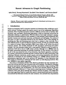
Fig. 1: Two dimensional examples for the eight base relations of RCC-8 sets of some topological space by stating their topological relations to each other. RCC-8 is the constraint language formed by the following 8 binary topological relations of RCC: disconnected (DC), externally connected (EC), equal (EQ), partially overlapping (P O), tangential proper part (T P P ), tangential proper part inverse (T P P I), nontangential proper part (N T P P ), and non-tangential proper part inverse (N T P P I). These eight relations are depicted in Figure 1 (2D case). It has come to our attention that the real case scenario, real world, datasets we are particularly interested in correspond to graphs with a scale-free-like structure, i.e., the degree distribution of the graphs follows a power law. Scale-free graphs seem to match real world applications well and are widely observed in natural and human-made systems, including the Internet, the World Wide Web, and the Semantic Web [5]–[8]. We argue that the case of scale-free graphs applies also to qualitative spatial networks and we stress on the importance of being able to efficiently reason with such scale-free-like networks for the following two main reasons: •

The natural approach for describing topological relations inevitably leads to the creation of graphs that exhibit hubs for particular objects which are cited more than others due to various reasons, such as size, significance, and importance. These hubs are in fact the most notable characteristic in scale-free graphs [5], [6]. For example, if we were to describe the topological relations in Greece, Greece would be our major hub that would relate topologically to all of its regions and cities, followed by smaller hubs that would capture topological relations within the

premises of a city or a neighborhood. It would not really make sense to specify that the porch of a house is located inside Greece, when it is already encoded that the house is located inside a city of Greece. Such natural and humanmade systems are most often described by scale-free graphs [5]–[8]. • Real qualitative spatial datasets that are known today, such as the ones used in [9]1 which we also use here, come from the Semantic Web, also called Web of Data, which is argued to be scale-free [7]. Further, more real datasets are to be offered by the Semantic Web community as RCC-8 has already been adopted by GeoSPARQL [3], and there is an ever increasing interest in coupling qualititave spatial reasoning techniques with linked geospatial data that are constantly being made available [10], [11]. Thus, there is a real need for scalable implementations of constraint network algorithms for qualitative and quantitative spatial constraints as RDF stores supporting linked geospatial data are expected to scale to billions of triples [10], [11]. In literature, the state-of-the-art techniques for tackling such large networks employ the following two approaches for retaining the sparseness of their underlying graphs and reasoning with them: (i) graph triangulation and sparse matrix implementation, and (ii) graph partitioning and parallelization. Regarding the first approach, a simple solution has been presented in [12] that utilizes a hash table based adjacency list to fit and reason with an underlying chordal graph of the large input network. Regarding the latter approach, a more complex implementation has been offered by Nikolaou and Koubarakis in [9], that employs graph partitioning to reduce the initial size of the large input network and exploits the degree of parallelism offered by current computer architectures by checking consistency of these smaller subnetworks in parallel. Due to improper use of the competing solvers, the authors of [9] obtained the wrong conclusion that their implementation is able to provide fast consistency for very large qualitative spatial networks with respect to the state-of-the-art. In particular, and as we will analyse further in our experimental evaluation in Section IV, the authors used outdated and inappropriate solvers, wrong flags for competitive solvers, and tree inputs for algorithms that rely on 3-cliques (triangles) to operate on. Thus, their implementation was in a race against itself. In this paper, we concentrate on the consistency checking problem of large scale-free-like qualitative spatial networks and make the following contributions: (i) we review the two aforementioned approaches and contradict the results of Nikolaou and Koubarakis in [9] by properly re-evaluating them with the benchmark dataset of that paper, (ii) we establish a clear view on the state-of-the-art solutions for reasoning with large real world qualitative spatial networks efficiently. It is important to note, that we do not dispute 1 http://cgi.di.uoa.gr/∼charnik/oss/gp-rcc8/

the concept of graph partitioning with parallelization for fast consistency checking of very large real world RCC-8 networks altogether, but just state the mere fact that the implementation in [9] fails, if anything, to support it, while misleading in an attempt to do so. The organization of this paper is as follows. Section II formally introduces the RCC-8 constraint language, chordal graphs along with the triangulation procedure, and graph partitioning. In Section III we briefly overview the state-ofthe-art solutions that make use of triangulation and graph partitioning, but also competitive ones that do not make use of these techniques. In Section IV we experimentally evaluate all proposed solutions for tackling very large real world RCC-8 networks with the real dataset benchmark used in [9]1 , and, finally, in Section V we conclude. We assume that the reader is familiar with the concepts of constraint networks and their corresponding constraint graphs that are not defined explicitly in this paper due to space constraints. Also, in what follows, we will refer to undirected graphs simply as graphs and we will use the terms real world and scale-free-like interchangeably. II. P RELIMINARIES In this section we formally introduce the RCC-8 constraint language, chordal graphs along with the triangulation procedure, and graph partitioning. The RCC-8 constraint language: A (binary) qualitative temporal or spatial constraint language [13] is based on a finite set B of jointly exhaustive and pairwise disjoint (JEPD) relations defined on a domain D, called the set of base relations. The set of base relations B of a particular qualitative constraint language can be used to represent definite knowledge between any two entities with respect to the given level of granularity. B contains the identity relation Id, and is closed under the converse operation (−1 ). Indefinite knowledge can be specified by unions of possible base relations, and is represented by the set containing them. Hence, 2B represents the total set of relations. 2B is equipped with the usual set-theoretic operations union and intersection, the converse operation, and the weak composition operation. The converse of a relation is the union of the converses of its base relations. The weak composition  of two relations s and t for a set of base relations B is defined as the strongest relation r ∈ 2B which contains s ◦ t, or formally, s  t = {b ∈ B | b ∩(s ◦ t) 6= ∅}, where s ◦ t = {(x, y) | ∃z : (x, z) ∈ s ∧ (z, y) ∈ t} is the relational composition [13], [14]. In the case of the qualitative spatial constraint language RCC-8 [4], as already mentioned in Section I, the set of base relations is the set {DC,EC,P O,T P P ,N T P P ,T P P I,N T P P I,EQ}, with EQ being the identity relation (Figure 1). Definition 1: An RCC-8 network comprises a pair (V, C) where V is a non-empty finite set of variables and C is a

0

1

2

3

4

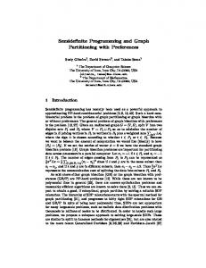
Fig. 2: Example of a chordal graph mapping that associates a relation C(v, v 0 ) ∈ 2B to each pair (v, v 0 ) of V × V . C is such that C(v, v) ⊆ {EQ} and C(v, v 0 ) = (C(v 0 , v))−1 . In what follows, C(vi , vj ) will be also denoted by Cij . Checking the consistency of a RCC-8 network is N Phard in general [15]. However, there exist large maximal tractable subclasses of RCC-8 which can be used to make reasoning much more efficient even in the general N Phard case. These maximal tractable subclasses of RCC-8 ˆ 8 , C8 , and Q8 [16]. Given a RCC-8 network are the sets H N = (V, C), consistency checking is then realised by a path consistency algorithm that iteratively performs the following operation until a fixed point C is reached: ∀i, j, k, Cij ← Cij ∩ (Cik  Ckj ), where variables i, k, j form triangles that belong either to a completion [17] or a chordal completion [18] of the underlying graph of the input network. Within the operation, weak composition of relations is aided by the weak composition table for RCC-8 [19]. If Cij = ∅ for a pair (i, j) then N is inconsistent, otherwise N is path consistent. If the relations of the input RCC-8 network belong to ˆ 8 , C8 , and some tractable subclass of relations, such as H Q8 [16], path consistency implies consistency, otherwise a backtracking algorithm decomposes the initial relations into subrelations belonging to some tractable subclass of relations spawning a branching search tree [14]. Chordal graphs and Triangulation: We begin by introducing the definition of a chordal graph. The interested reader may find more results regarding chordal graphs, and graph theory in general, in [20]. Definition 2 ([20]): Let G = (V, E) be an undirected graph. G is chordal or triangulated if every cycle of length greater than 3 has a chord, which is an edge connecting two non-adjacent nodes of the cycle. The graph shown in Figure 2 consists of a cycle which is formed by five solid edges and two dashed edges that correspond to its chords. As for this part, the graph is chordal. However, removing one dashed edge would result in a non-chordal graph. Indeed, the other dashed edge with three solid edges would form a cycle of length four with no chords. Chordality checking can be done in (linear) O(|V | + |E|) time for a given graph G = (V, E) with the

maximum cardinality search algorithm which also constructs an elimination ordering α as a byproduct [21]. If a graph is not chordal, it can be made so by the addition of a set of new edges, called fill edges. This process is usually called triangulation of a given S graph G = (V, E) and can run as fast as in O(|V |+(|E F (α)|)) time, where F (α) is the set of fill edges that result by following the elimination ordering α, eliminating the nodes one by one, and connecting all nodes in the neighborhood of each eliminated node, thus, making it simplicial in the elimination graph. If the graph is already chordal, following the elimination ordering α means that no fill edges are added, i.e., α is actually a perfect elimination ordering [20]. For example, a perfect elimination ordering for the chordal graph shown in Figure 2 would be the ordering 1 → 3 → 4 → 2 → 0 of its set of nodes. In general, it is desirable to achieve chordality with as few fill edges as possible. However, obtaining an optimum graph triangulation is known to be N P-hard [21]. In a RCC-8 network fill edges correspond to universal relations, i.e., nonrestrictive relations that contain all base relations. Chordal graphs become relevant in the context of qualitative spatial reasoning due to the following result obtained in [18] that states that path consistency enforced on the underlying chordal graph of an input network can yield consistency of the input network: Proposition 1 ([18]): For a given RCC-8 network N = (V, C) with relations from the maximal tractable subclasses ˆ 8 , C8 , and Q8 and for G = (V, E) its underlying chordal H graph, if ∀(i, j), (i, k), (j, k) ∈ E we have that Cij ⊆ Cik  Ckj , then N is consistent. Chordal graphs suit sparse graphs with clustering properties, such as scale-free graphs, particularly well [12]. We are about to experimentally verify this in Section IV. Graph Partitioning: Given a graph G, the graph partitioning problem concerns the partitioning of G into smaller components with specific properties. For instance, a k-way partitioning divides the vertex set into k smaller components. A good partitioning is defined as one in which the number of edges running between separated components is small. Important applications of graph partitioning include scientific computing, partitioning various stages of a VLSI design circuit, task scheduling in multi-processor systems, and clustering and detection of cliques in social, pathological, and biological networks [22], [23]. Graph partitioning problems fall under the category of N P-hard problems [24], and solutions to these problems are generally derived using heuristics and approximation algorithms, such as the ones offered by the METIS2 software [25] employed in [9]. In [9], the authors define the notion of a partitioning graph, where they require (among other things) that the smaller components into which the underlying graph G of a 2 http://glaros.dtc.umn.edu/gkhome/metis/metis/overview

networks.

0

1

2

3

0

4

0

0

1

2

3

3

4

4

Fig. 3: Example of a partitioning graph [9] given RCC-8 network is partitioned, are augmented, where appropriate, with endpoints of edges that run across them and completed through the introduction of fill edges, so that path consistency can be enforced on them and a complete agreement on the overlapping part of two components with respect to their corresponding solutions can be verified, much like as in [26]. For example, in Figure 3, the 3-way partitioning graph of an initial graph is depicted, along with the introduction of (dashed) fill edges that complete the separate components. The observant reader will notice that such a partitioning graph is a particular case of a tree decomposition [27] of a chordal graph, since a chordal graph yields a natural tree decomposition of its cliques in linear time [20]. In fact, if one patches together the components shown in Figure 3, he will obtain the chordal graph depicted in Figure 2. This comes as no surprise, as both the works of Huang et al. [26] (where a structure called dtree is enlisted) and Nikolaou et al. [9] employ a particular theoretical property that relies on tree decompositions to guarantee soundness and completeness. As an example, omitting path consistency checks across children of dtree nodes [26] corresponds to omitting those checks across clusters of the tree decomposition into which the dtree is converted, as has been specifically pointed out in [28]. Intuitively, tree decompositions are used as a requirement of acyclicity of cliques. Thus, the authors in [9] implicitly consider Proposition 1. However, the use of graph partitioning in this case still makes sense when one wants to impose additional properties on the components, such as restraining their size or reducing the number of edges different components share between one another. III. OVERVIEW OF STATE - OF - THE - ART TOOLS In this section we review the state-of-the-art solutions that exist for tackling very large large scale-free-like RCC-8

Sarissa: We have implemented Sarissa3 in Python, that is the latest updated, generalised, and code refactored version of PyRCC85 originally presented in [18]. Sarissa supports small arbitrary binary constraint calculi developed for spatial and temporal reasoning for which Proposition 1 holds, such as RCC-8 and Allen’s interval algebra (IA) [29], in a way similar to GQR [30]. Further, Sarissa presents significant improvements over PyRCC85 regarding functionality, scalability, and speed. In particular, Sarissa opts for a hash table based adjacency list as a sparse matrix implementation to represent and reason with the chordal completion of the input network. The variables of the input network (or the nodes) are represented by index numbers of a list, and each variable (or node) is associated with a hash table that stores key-value pairs of variables and relations. For a given RCC-8 network N = (V, C) and for G = (V, E) its underlying chordal graph, our approach requires O(|V | + |E| · b) memory, where b is the size needed to represent a relation from the set of relations 2B of RCC-8. Further, we still retain an O(1) average access and update time complexity which becomes O(δ) in the amortized worst case, where δ is the average degree of a chordal graph that corresponds to the input network. Given that we target large scale-free-like, and, thus, sparse networks [31], this only incures a small penalty for the related experiments performed. The path consistency implementation also benefits from this approach as the queue data structure which is based on has to use only O(|E|) of memory to store the relations. Regarding triangulation, the hash table based adjacency list is coupled with the implementation of the maximum cardinality search algorithm and a fast fill in procedure (as discussed in Section II), as opposed to the heuristic based, but rather naive, triangulation procedure implemented in [18]. Though the maximum cardinality search algorithm does not yield minimal triangulations if the underlying graph of the input network is not chordal, it does guarantee than no fill edges are inserted if the graph is indeed chordal. In addition, even for the non-chordal cases we obtain good results with this approach and have a fine trade-off between time efficiency and good triangulations. Sarissa is a generic and open source qualitative reasoner and it was shown to improve the stateof-the-art techniques for tackling large scale-free-like RCC-8 networks in [12]. gp-rcc8: Reasoner gp-rcc81 is written in C++ and was introduced in [9] for tackling very large scale-freelike RCC-8 networks. It employs graph partitioning through the use of METIS2 to reduce the initial size of the network by decomposing it into k smaller subnetworks and exploits the degree of parallelism offered by current computer architectures by checking consistency of these smaller 3 http://www.cril.fr/∼sioutis/work.php

subnetworks in a parallel fashion. Graph partitioning alone imposes a significant overhead since it falls under the category of N P-hard problems (as discussed in Section II). Path consistency is enforced by filtering each subnetwork, merging and intersecting relations that belong to intersecting subnetworks, and repeating the procedure until a fixpoint is reached. Regarding consistency checking, and since there can be exponentially many refinements of the relations of a subnetwork into relations belonging to some of the ˆ 8 , C8 , and Q8 , maximal tractable subclasses of relations H things get more complicated, as one needs to find the refinements that agree on the common parts between the subnetworks to be able to apply Proposition 1. The solution to this as presented in [9] is to find candidate refinements of all relations belonging to the common parts between subnetworks into base relations and then move on with checking the consistency of the different subnetworks of the partitioning graph independently. Thus, gp-rcc8 does not fully take advantage of the maximal tractable subclasses ˆ 8 , C8 , and Q8 , and the use of base relations of relations H may explode the search space under circumstances. The implementation builds on the reasoning engine of the solver presented in [17] and its performance depends on the choice of parameters for the partitioning strategy, but also on the number of k parts one would like to acquire. Objectively, this constitutes a limitation regarding the practical use of the software as it is almost impossible to get the optimal combination of parameters on the first run and the sensitivity of parameters is relatively high [9, Fig. 2a-b]. In the experimental evaluation to follow in Section IV we made several runs to obtain a near global minimum regarding its performance. GQR: Generic Qualitative Reasoner (GQR4 ) [30] is a solver for binary qualitative constraint networks, that supports arbitrary binary constraint calculi developed for spatial and temporal reasoning, such as the calculi from the RCC family, and Allen’s interval algebra (IA) [29]. GQR uses a hand-written queue put together from generic components (parts of the C++ Standard Template Library STL), implemented as a virtual class, allowing for easy and convenient extensions. GQR also employs hash tables and different methods for creating and handling precomputations of composition and converse tables. GQR is implemented in C++ and makes extensive use of templates. Although it does not employ triangulation or graph partitioning and builds on a matrix representation that forbids it from being able to represent large networks of millions of nodes, it remains a very competitive solver within its range [12]. This is due to being under active development for several years and incorporating advanced reasoning techniques, such as restart and nogood recording [32]. 4 http://sfbtr8.informatik.uni-freiburg.de/R4LogoSpace/Tools/gqr.html

IV. E XPERIMENTAL EVALUATION In this section, we evaluate reasoners Sarissa3 under version 0.2-beta, gp-rcc81 under version 0.2-alpha, and GQR4 under version 1500 (all accessed at 2014-07-09) with the real dataset used in [9]1 , and show that gp-rcc8 complements the state-of-the-art regarding enforcing path consistency and falls very short regarding consistency checking, thus, contradicting the conclusion drawn in [9] about being able to provide fast consistency checking for very large real world datasets. First, we briefly overview the improper use of competing solvers in [9] that resulted in that conclusion: (i) GQR was employed without the flag that allows it to use the ˆ 8 , as a result, GQR would try to maximal tractable subclass H instantiate up to (n·(n−1))/2 variables using base relations for a network of n nodes, even if only a few relations existed ˆ 8 (e.g., for 10 such relations that were not included in H GQR would initially consider 10 variables, plus, relation B, the universal non-restrictive relation containing all base reˆ 8 and does not have to be split at all). (ii) lations, exists in H The outdated solver PyRCC85 was used under the version it appeared in [18], and not under any other version we kept regularly updated in our website, with Sarissa being its latest update as a generic solver, available online since 2013. (iii) Solver rcc8sat [26] was used for tackling tractable networks of thousands of nodes [9, Tab. 1], when it was shown in [26] that it is only appropriate and complements the stateof-the-art when needing to solve very hard network instances of up to 150-200 nodes, thus, an argument could be made about that with a small evaluation on the side if necessary. The result in [9] is still positive information, but somewhat expected and adds to the improper use of adverse solvers that change the overall conclusion. (iv) Accompanying the real dataset to be used also in this paper, there was a synthetic dataset of networks where their underlying structure was a tree [9, Fig. 2c]. These networks are trivially consistent, they are chordal graphs without even triangles, thus, the evaluation was not about reasoning as path consistency was trivially employed (it needs 3-cliques to operate on), but about how fast a solver can go over the variables, keep the state in case of backtracking (that will never happen), apply heuristics for choosing the next variable (when one could pick a random one), until all variables are instatiated. Partitioning a n node tree in n − 1 parts and instatiating the corresponding variables in parallel, would always give you a benefit, especially in combination with the other three aforementioned issues (e.g., Sarrisa under its latest update only considers relations that belong to triangles in the obtained chordal graph, thus, it would mark the tree network consistent almost immediately without instatiating any variables, and GQR with the proper flag would initially consider n−1 variables instead of (n·(n−1))/2). As noted, the above issues resulted in gp-rcc8 being in a race against

Performance of three reasoners for nuts

102

Performance of three reasoners for adm1

105

Performance of three reasoners for gadm1

103

104

100

Elapsed real time (sec)

103

Elapsed real time (sec)

Elapsed real time (sec)

101

102 101

102

101

10-1 100 10-2

GQR

Sarissa

gp-rcc8

10-1

GQR

Sarissa

100

gp-rcc8

GQR

Sarissa

gp-rcc8

(a) Performance comparison for nuts (consistent) (b) Performance comparison for adm1 (consistent) (c) Performance comparison for gadm1 (inconsistent) Performance of three reasoners for gadm2c

100

Sarissa

GQR

gp-rcc8

101

100

Performance of three reasoners for adm2

103

Elapsed real time (sec)

101

Performance of three reasoners for gadm2

102

Elapsed real time (sec)

Elapsed real time (sec)

102

Sarissa

GQR

gp-rcc8

102

Sarissa

GQR

gp-rcc8

(d) Performance comparison for gadm2c (consistent)(e) Performance comparison for gadm2 (inconsistent) (f) Performance comparison for adm2 (consistent)

Fig. 4: Performance comparison for the path consistency operation

itself. Technical Specifications: The experiments were carried out on a computer with an Intel Core 2 Quad Q9400 processor (4 physical cores) with a CPU frequency of 2.66 GHz per core, 8 GB RAM, and the Precise Pangolin x86 64 OS (Ubuntu Linux). GQR and gp-rcc8 were compiled with gcc/g++ 4.6.3. Regarding gp-rcc8, the boost5 library under version 1.48 was also used. Sarissa was run with PyPy6 2.3.1, which fully implements Python 2.7.6. Only one of the CPU cores was used for GQR and Sarissa, and all four for gp-rcc8. Regarding the performance of gp-rcc8, the results represent its near global minimum in every case, as we ran the reasoner several times for different combinations of parameters to find the most appropriate one. In particular, for all experiments the minimum fringe strategy for partitioning the graph was the most appropriate. The optimal number of parts in combination with that strategy will be specified for every dataset in the discussion to follow. Regarding GQR and Sarissa the flag for using the maximal tractable subclass ˆ 8 was specified, and for Sarissa an additional flag to apply H a special heuristic was specified for the instances that were used to evaluate consistency checking performance (viz., -e

local). All measurements consider elapsed real time (wall clock time). Dataset: We consider the dataset of real network instances that was used in [9]1 , which we describe as follows: • nuts: a nomenclature of territorial units using RCC-8 relations that contains 2 235/3 176 nodes/edges.7 • adm1: a network that describes the administrative geography of Great Britain using RCC-8 relations [33] and contains 11 761/44 833 nodes/edges. • gadm1: a network that describes the german administrative units using RCC-8 relations and contains 42 749/159 600 nodes/edges. • gadm2: a network that describes the world’s (global) administrative areas using RCC-8 relations and contains 276 727/590 443 nodes/edges.8 • gadm2c: this is the same network as gadm2 with inconsistencies removed to make it consistent. • adm2: a network that describes the greek administrative geography using RCC-8 relations and contains 1 732 999/5 236 270 nodes/edges.7 The aforementioned network instances are tractable, and they also contain one or two base RCC-8 relations per edge. Instances for evaluating the consistency checking

5 http://www.boost.org/

7 Retrieved

6 http://pypy.org/

8 http://gadm.geovocab.org/

from: http://www.linkedopendata.gr/

100

10-1

104

Sarissa

GQR

gp-rcc8

Performance of three reasoners for hard-adm1

103

102

Sarissa

GQR

gp-rcc8

Performance of three reasoners for hard-gadm1

105

Elapsed real time (sec)

Performance of three reasoners for hard-nuts

Elapsed real time (sec)

Elapsed real time (sec)

101

104

103

Sarissa

GQR

gp-rcc8

(a) Performance comparison for hard-nuts (con-(b) Performance comparison for hard-adm1 (con-(c) Performance comparison for hard-gadm1 (insistent) sistent) consistent)

Fig. 5: Performance comparison for the consistency operation

performance of the reasoners were constructed in [9] with the introduction of N P 8 relations [17] in the networks’ edges. These instances are hard-nuts, hard-adm1, and hard-gadm1. We assess the performance of both path consistency enforcing and consistency checking for all reasoners. Path Consistency Enforcing: The results can be viewed in Figure 4. Regarding the medium to large sized instances nuts, adm1, and gadm1, gp-rcc8 is the clear winner with its most impressive performance being for adm1 where it manages to snap its inference costs and decide its consistency in 0.573 sec, when Sarissa needs 200.06 sec, and GQR 17 701.191 sec. Note that GQR, as opposed to Sarissa and gp-rcc8, enforces path consistency with respect to a complete underlying graph of the input network. To obtain this performance for gp-rcc8 we had to partition nuts, adm1, and gadm1 in 50, 250, and 500 parts respectively, after several runs. However, the tables turn regarding the very large sized instances gadm2, gadm2c, and adm2 which are decided in 4.217 sec, 5.930 sec, and 428.756 sec for Sarissa and in 18.291 sec, 17.698 sec, and 377.111 sec for gp-rcc8 respectively. GQR is of course not able to fit the networks in its matrix. Thus, Sarissa is 80% faster than gp-rcc8 for gadm2, 67% faster than gp-rcc8 for gadm2c, and 14% slower than gp-rcc8 for adm2. Again, we had to partition gadm2, gadm2c, and adm2 for gp-rcc8 in 2 700, 2 800, and 12 000 parts respectively, after several runs. Taking into account the results for the very large instances gadm2, gadm2c, and adm2, and keeping in mind that gp-rcc8 utilizes all four cores, whereas Sarissa only one, and that it is impossible to guess the correct parameters for gp-rcc8 a priori, it is fair to argue that gp-rcc8 does not improve the state-of-the-art regarding path consistency enforcing on very large real world networks, but complements it at best. In fact, only the time to partition gadm2 and gadm2c (around 10 sec) was already over the time for Sarissa to load,

triangulate, and reason with the network. The same situation applies for adm2 where partitioning its graph took around 5 minutes in our machine. These measurements establish a lower bound for gp-rcc8 that is close to the performance of Sarissa, which could even utilize more aggresive (non-linear) triangulation in case needed. Consistency Checking: For the given dataset, this experiment utilizes the whole reasoning engine of a reasoner, as both path consistency and some algorithm to realise backtracking search need to be employed. As noted, hard instances where constructed with the introduction of N P 8 relations [17] in the networks’ edges. The results can be viewed in Figure 5, where one can see that gp-rcc8 is only able to tackle the first and smallest of all instances, namely, hard-nuts, in a little less than a second. We had to partition hard-nuts for gp-rcc8 in 100 parts. In fact, this instance was easy for all reasoners to tackle, even for GQR who spend most of its time initializing a big matrix. We were not able to receive an answer from gp-rcc8 regarding hard-adm1 as it hit the 8 GB memory limit after ∼ 10 minutes. We can only refer to the result in [9] which was obtained in a similar machine (4-core 2.4 GHz CPU, 64 GB RAM) that states a time of 13 091.96 sec. Sarissa and GQR solve this instance in 173.974 sec and 4 901.023 sec respectively, thus, both Sarissa and GQR are a lot faster. We were not able to receive an answer from gp-rcc8 regarding hard-gadm1 either, even though Sarissa and GQR comfortably solve the network in 2 557.714 sec and 14 357.267 sec respectively. Referring again to the result in [9], gp-rcc8 was unable to offer an answer in the 64 GB test machine too. It is clear at this point, and with respect to the given dataset, that gp-rcc8 falls very short regarding the state-of-the-art in checking the consistency of very large networks with a real world structure, which is a contradiction to what has been concluded in [9]. We must also state that Sarissa is only a simple implementation with a triangulation algorithm and a sparse matrix implementation

that any solver, such as GQR, can easily adopt. V. C ONCLUSION In this paper, we established a clear view on the stateof-the-art solutions for reasoning with large real world qualitative spatial networks efficiently, by re-evaluating them with the benchmark dataset of [9], providing new results that contradict the results of that paper with respect to that dataset. As noted in our introduction, it is important to remind the reader that we do not dispute the concept of graph partitioning with parallelization for fast consistency checking of very large real world RCC-8 networks altogether, but just show that due to improper use of competing solvers the implementation in [9] does not currently support it. However, the implementation in [9] looks promising and with space for improvement, and calls for further research. Acknowledgements: This work was funded by a PhD grant from Universit´e d’Artois and region Nord-Pas-deCalais. We would also like to thank Matthias Westphal and Jason Jingshi Li for providing useful feedback on an earlier draft of this paper, and for fruitful discussions in general. R EFERENCES [1] S. Hazarika, Qualitative Spatio-Temporal Representation and Reasoning: Trends and Future Directions. Igi Global, 2012. [2] M. Koubarakis and K. Kyzirakos, “Modeling and Querying Metadata in the Semantic Sensor Web: The Model stRDF and the Query Language stSPARQL,” in ESWC, 2010. [3] Open Geospatial Consortium, “OGC GeoSPARQL - A geoR graphic query language for RDF data,” OGC Implementation Standard, 2012. [4] D. A. Randell, Z. Cui, and A. Cohn, “A Spatial Logic Based on Regions and Connection,” in KR, 1992. [5] A.-L. Barabasi and E. Bonabeau, “Scale-Free Networks,” Scientific American, pp. 50–59, 2003. [6] O. Hein, M. Schwind, and W. Knig, “Scale-Free Networks - The Impact of Fat Tailed Degree Distribution on Diffusion and Communication Processes,” Wirtschaftsinformatik, vol. 47, pp. 21–28, 2006. [7] M. Steyvers and J. B. Tenenbaum, “The Large-Scale Structure of Semantic Networks: Statistical Analyses and a Model of Semantic Growth,” Cognitive Science, vol. 29, pp. 41–78, 2005. [8] A. L. Barabasi and R. Albert, “Emergence of scaling in random networks,” Science (New York, N.Y.), vol. 286, pp. 509–512, 1999. [9] C. Nikolaou and M. Koubarakis, “Fast Consistency Checking of Very Large Real-World RCC-8 Constraint Networks,” in AAAI, 2014. [10] M. Koubarakis, K. Kyzirakos, M. Karpathiotakis, C. Nikolaou, M. Sioutis, S. Vassos, D. Michail, T. Herekakis, C. Kontoes, and I. Papoutsis, “Challenges for Qualitative Spatial Reasoning in Linked Geospatial Data,” in BASR, 2011. [11] C. Nikolaou and M. Koubarakis, “Querying Incomplete Geospatial Information in RDF,” in SSTD, 2013.

[12] M. Sioutis and J.-F. Condotta, “Tackling Large Qualitative Spatial Networks of Scale-Free-Like Structure,” in SETN, 2014, pp. 178–191. [13] J. Renz and G. Ligozat, “Weak Composition for Qualitative Spatial and Temporal Reasoning,” in CP, 2005. [14] J. Renz and B. Nebel, “Qualitative Spatial Reasoning Using Constraint Calculi,” in Handbook of Spatial Logics, 2007, pp. 161–215. [15] ——, “Spatial Reasoning with Topological Information,” in Spatial Cognition, 1998. [16] J. Renz, “Maximal Tractable Fragments of the Region Connection Calculus: A Complete Analysis,” in IJCAI, 1999. [17] J. Renz and B. Nebel, “Efficient Methods for Qualitative Spatial Reasoning,” JAIR, vol. 15, pp. 289–318, 2001. [18] M. Sioutis and M. Koubarakis, “Consistency of Chordal RCC8 Networks,” in ICTAI, 2012. [19] S. Li and M. Ying, “Region connection calculus: Its models and composition table,” Artif. Intell., vol. 145, pp. 121–146, 2003. [20] M. C. Golumbic, Algorithmic Graph Theory and Perfect Graphs, 2nd ed. Elsevier Science, 2004. [21] A. Berry, J. R. S. Blair, and P. Heggernes, “Maximum Cardinality Search for Computing Minimal Triangulations,” in WG, 2002. [22] K. Andreev and H. R¨acke, “Balanced Graph Partitioning,” Theory Comput. Syst., vol. 39, pp. 929–939, 2006. [23] A. Buluc¸, H. Meyerhenke, I. Safro, P. Sanders, and C. Schulz, “Recent Advances in Graph Partitioning,” CoRR, vol. abs/1311.3144, 2013. [24] M. R. Garey, D. S. Johnson, and L. J. Stockmeyer, “Some Simplified NP-Complete Graph Problems,” Theor. Comput. Sci., vol. 1, pp. 237–267, 1976. [25] G. Karypis and V. Kumar, “Multilevel k-way Hypergraph Partitioning,” in DAC, 1999, pp. 343–348. [26] J. Huang, J. J. Li, and J. Renz, “Decomposition and tractability in qualitative spatial and temporal reasoning,” Artif. Intell., pp. 140–164, 2013. [27] N. Robertson and P. D. Seymour, “Graph minors. III. Planar tree-width,” J. Comb. Theory, Ser. B, vol. 36, pp. 49–64, 1984. [28] J. Condotta and D. D’Almeida, “Consistency of Qualitative Constraint Networks from Tree Decompositions,” in Eighteenth International Symposium on Temporal Representation and Reasoning, TIME 2011, L¨ubeck , Germany, September 12-14, 2011, 2011, pp. 149–156. [29] J. F. Allen, “Maintaining knowledge about temporal intervals,” CACM, vol. 26, pp. 832–843, 1983. [30] Z. Gantner, M. Westphal, and S. W¨olfl, “GQR-A Fast Reasoner for Binary Qualitative Constraint Calculi,” in AAAI Workshop on Spatial and Temporal Reasoning, 2008. [31] C. I. Del Genio, T. Gross, and K. E. Bassler, “All Scale-Free Networks Are Sparse,” Phys. Rev. Lett., vol. 107, p. 178701, 2011. [32] M. Westphal, S. W¨olfl, and J. J. Li, “Restarts and Nogood Recording in Qualitative Constraint-based Reasoning,” in ECAI, 2010. [33] J. Goodwin, C. Dolbear, and G. Hart, “Geographical Linked Data: The Administrative Geography of Great Britain on the Semantic Web,” TGIS, vol. 12, pp. 19–30, 2008.