High Quality Graph Partitioning ⋆

High Quality Graph Partitioning ? Peter Sanders, Christian Schulz Karlsruhe Institute of Technology, 76128 Karlsruhe, Germany {sanders, christian.schulz}@kit.edu

Abstract. We present an overview over our graph partitioners KaFFPa (Karlsruhe Fast Flow Partitioner) and KaFFPaE (KaFFPa Evolutionary). KaFFPa is a multilevel graph partitioning algorithm which on the one hand uses novel local improvement algorithms based on max-flow and min-cut computations and more localized FM searches and on the other hand uses more sophisticated global search strategies transferred from multi-grid linear solvers. KaFFPaE is a distributed evolutionary algorithm to solve the Graph Partitioning Problem. KaFFPaE uses KaFFPa which provides new effective crossover and mutation operators. By combining these with a scalable communication protocol we obtain a system that is able to improve the best known partitioning results for many inputs.

1

Introduction

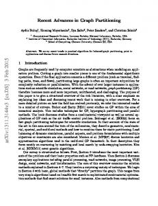
Problems of graph partitioning arise in various areas of computer science, engineering, and related fields. For example in route planning, community detection in social networks and high performance computing. In many of these applications large graphs need to be partitioned such that there are few edges between blocks (the elements of the partition). For example, when you process a graph in parallel on k processors you often want to partition the graph into k blocks of about equal size so that there is as little interaction as possible between the blocks. In this paper we focus on a version of the problem that constrains the maximum block size to (1 + ) times the average block size and tries to minimize the total cut size, i.e., the number of edges that run between blocks. It is well known that this problem is NP-complete [5] and that there is no approximation algorithm with a constant ratio factor for general graphs [5]. Therefore mostly heuristic algorithms are used in practice. A successful heuristic for partitioning large graphs is the multilevel graph partitioning (MGP) approach depicted in Figure 1 where the graph is recursively contracted to achieve smaller graphs which should reflect the same basic structure as the input graph. After applying an initial partitioning algorithm to the smallest graph, the contraction is undone and, at each level, a local refinement method is used to improve the partitioning induced by the coarser level. Although several successful multilevel partitioners have been developed in the last 13 years, we had the impression that certain aspects of the method are not well understood. We therefore have built our own graph partitioner KaPPa [14] (Karlsruhe Parallel Partitioner) with focus on scalable parallelization. Somewhat astonishingly, we also obtained improved partitioning quality through rather simple methods. This motivated us ?

Partially supported by DFG SA 933/10-1.

2 2.1

refinement phase

contraction phase

to make a fresh start putting all aspects of MGP on trial. This paper gives an overview over our most recent work, KaFFPa [23] and KaFFPaE [22]. KaFFPa is a classical matching based graph partitioning algorithm with focus on local improvement methods and overall search strategies. It is a system that can be configured to either achieve the best known partitions for many standard benchmark instances or to be the fastest available system for large graphs while still improving partitioning quality compared to the previous fastest system. KaFFPaE is a technique which integrates an evolutionary search algorithm with our multilevel graph partitioner KaFFPa and its scalable parallelization. It uses novel mutation and combine operators which in contrast to previous evolutionary methods that use a graph partitioner [24, 8] do not need random perturbations of edge weights. The combine operators enable us to combine individuals of different kinds (see Section 5 for more details). Due to the parallelization our system is able to compute partitions that have quality comparable or better than previous entries in Walshaw’s well known partitioning benchmark within a few minutes for graphs of moderate size. Previous methods of Soper et. al [24] required runtimes of up to one week for graphs of that size. We therefore believe that in contrast to previous methods, our method is very valuable in the area of high performance computing. The paper is organized as follows. We beinput output gin in Section 2 by introducing basic congraph partition cepts which is followed by related work ... ... local improvement match in Section 3. In Section 4 we present the techniques used in the multilevel graph contract uncontract initial partitioner KaFFPa. We continue describing the main components of our evolupartitioning tionary algorithm KaFFPaE in Section 5. Fig. 1. Multilevel graph partitioning. A summary of extensive experiments to evaluate the performance of the algorithm is presented in Section 6. We have implemented these techniques in the graph partitioner KaFFPaE (Karlsruhe Fast Flow Partitioner Evolutionary) which is written in C++. Experiments reported in Section 6 indicate that KaFFPaE is able to compute partitions of very high quality and scales well to large networks and machines.

Preliminaries Basic concepts

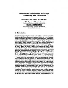
Consider an undirected graph G = (V, E, c, ω) with edge weights ω : E → R>0 , node weights |, and m = |E|. We extend c and ω to sets, i.e., P c : V → R≥0 , n = |VP c(V 0 ) := v∈V 0 c(v) and ω(E 0 ) := e∈E 0 ω(e). Γ (v) := {u : {v, u} ∈ E} denotes the neighbors of v. We are looking for blocks of nodes V1 ,. . . ,Vk that partition V , i.e., V1 ∪ · · · ∪ Vk = V and Vi ∩ Vj = ∅ for i 6= j. The balancing constraint demands that ∀i ∈ {1..k} : c(Vi ) ≤ Lmax := (1 + )c(V )/k + maxv∈V c(v) for some parameter . The last term in this equation arises because each node is atomic and therefore a deviation P of the heaviest node has to be allowed. The objective is to minimize the total cut i 1 is another parameter. The core is then temporarily contracted to a single vertex s and the ring into a single vertex t to compute the minimum s-t-cut between them using the given edge weights as capacities. To assure that every vertex eventually belongs to at least one Fig. 6. On the top we see the compucore, and therefore is inside at least one cut, the tation of a natural cut. A BFS Tree vertices v are picked uniformly at random among which starts from v is grown. The gray all vertices that have not yet been part of any core area is the core. The dashed line is the in any round. The process is stopped when there natural cut. It is the minimum cut between the contracted versions of the are no such vertices left. core and the ring (shown as the solid In the original work [8] each connected com- line). During the computation several ponent of the graph GC = (V, E\C), where C is natural cuts are detected in the input the union of all edges cut by the process above, is graph (bottom). contracted to a single vertex. Since we do not use v

9

natural cuts as a preprocessing technique at this place we don’t contract these components. Instead we build a clustering C of G such that each connected component of GC is a block. This technique yields the third instantiation of the combine framework C3 which is divided into two stages, i.e. the clustering used for this combine step is dependent on the stage we are currently in. In both stages the partition P used for the combine step is selected from the population using tournament selection. During the first stage we choose f uniformly at random in [5, 20], α uniformly at random in [0.75, 1.25] and we set U = |V |/3k. Using these parameters we obtain a clustering C of the graph which is then used in the combine framework described above. This kind of clustering is used until we reach an upper bound of ten calls to this combine step. When the upper bound is reached we switch to the second stage. In this stage we use the clusterings computed during the first stage, i.e. we extract elementary natural cuts and use them to quickly compute new clusterings. An elementary natural cut (ENC) consists of a set of cut edges and the set of nodes in its core. Moreover, for each node v in the graph, we store the set of ENCs N (v) that contain v in their core. With these data structures its easy to pick a new clustering C (see Algorithm 2) which is then used in the combine framework described above. Algorithm 2 computeNaturalCutClustering (second stage) 1: unmark all nodes in V 2: for each v ∈ V in random order do 3: if v is not marked then 4: pick a random ENC C in N (v) 5: output C 6: mark all nodes in C’s core

5.2

Mutation Operators

We define two mutation operators, an ordinary and a modified F-cycle. Both mutation operators use a random individual from the current population. The main idea is to iterate coarsening and refinement several times using different seeds for random tie breaking. The first mutation operator M1 can assure that the quality of the input partition does not decrease. It is basically an ordinary F-cycle which is an algorithm used in KaFFPa. Edges between blocks are not contracted. The given partition is then used as initial partition of the coarsest graph. In contrast to KaFFPa, we now can use the partition as input to the partition in the very beginning. This ensures nondecreasing quality since our refinement algorithms guarantee no worsening. The second mutation operator M2 works quite similar with the small difference that the input partition is not used as initial partition of the coarsest graph. That means we obtain very good coarse graphs but we cannot assure that the final individual has a higher quality than the input individual. In both cases the resulting offspring is inserted into the population using the eviction strategy described in Section 5.1. 5.3

Putting Things Together and Parallelization

We now explain the parallelization and describe how everything is put together. Each processing element (PE) basically performs the same operations using different random 10

seeds (see Algorithm 3). First we estimate the population size S: each PE performs a partitioning step and measures the time t spent for partitioning. We then choose S such that the time for creating S partitions is approximately ttotal /f where the fraction f is a tuning parameter and ttotal is the total running time that the algorithm is given to produce a partition of the graph. Each PE then builds its own population, i.e. KaFFPa is called several times to create S individuals/partitions. Afterwards the algorithm proceeds in rounds as long as time is left. With corresponding probabilities, mutation or combine operations are performed and the new offspring is inserted into the population. We choose a parallelization/communication protocol that is quite similar to randomized rumor spreading [9]. Let p denote the number of PEs used. A communication step is organized in rounds. In each round, a PE chooses a communication partner and sends her the currently best partition P of the local population. The selection of the communication partner is done uniformly at random among those PEs to which P not already has been sent to. Afterwards, a PE checks if there are incoming individuals and if so inserts them into the local population using the eviction strategy described above. If P is improved, all PEs are again eligible. This is repeated log p times. Note that the algorithm is implemented completely asynchronously, i.e. there is no need for a global synchronisation. The process of creating individuals is parallelized as follows: Each PE makes s0 = |S|/p calls to KaFFPa using different seeds to create s0 individuals. Afterwards we do the following S − s0 times: The root PE computes a random cyclic permutation of all PEs and broadcasts it to all PEs. Each PE then sends a random individual to its successor in the cyclic permutation and receives a individual from its predecessor in the cyclic permutation which is then inserted into the local population. When this particular part of the algorithm (quick start) is finished, each PE has |S| partitions. After some experiments we fixed the ratio of mutation to crossover operations to 1 : 9, the ratio of the mutation operators M1 : M2 to 4 : 1 and the ratio of the combine operators C1 : C2 : C3 to 3 : 1 : 1. Note that the communication step in the last line of the algorithm could also be performed only every x iterations (where x is a tuning parameter) to save communication time. Since the communication network of our test system is very fast (see Section 6), we perform the communication step in each iteration. Algorithm 3 All PEs perform the same operations using different random seeds. procedure locallyEvolve estimate population size S while time left if elapsed time < ttotal /f then create individual and insert into local population else flip coin c with corresponding probabilities if c shows head then perform a mutation operation else perform a combine operation insert offspring into population if possible communicate according to communication protocol

11

6

Experiments

Implementation. We have implemented the algorithm described above using C++. Overall, our program (including KaFFPa) consists of about 22 500 lines of code. We use two base case partitioners, KaFFPaStrong and KaFFPaEco. KaFFPaEco is a good tradeoff between quality and speed, and KaFFPaStrong is focused on quality (see [23] for more details).

graph n m Random Geometric Graphs rgg16 216 ≈342 K rgg17 217 ≈ 729 K Delaunay delaunay16 216 ≈ 197 K delaunay17 217 ≈ 393 K Kronecker G500 kron simple 16 216 ≈ 2 M kron simple 17 217 ≈ 5 M Numerical adaptive ≈6 M ≈14 M channel ≈5 M ≈42 M venturi ≈4 M ≈8 M packing ≈2 M ≈17 M 2D Frames hugetrace-00000 ≈5 M ≈7 M hugetric-00000 ≈6 M ≈9 M Sparse Matrices af shell9 ≈500 K ≈9 M thermal2 ≈1 M ≈4 M Coauthor Networks coAutCiteseer ≈227 K ≈814 K coAutDBLP ≈299 K ≈978 K Social Networks cnr ≈326 K ≈3 M caidaRouterLvl ≈192 K ≈609 K Road Networks luxembourg ≈144 K ≈120 K belgium ≈1 M ≈2 M netherlands ≈2 M ≈2 M italy ≈7 M ≈7 M great-britain ≈8 M ≈8 M germany ≈12 M ≈12 M asia ≈12 M ≈13 M europe ≈51 M ≈54 M

Systems. Experiments have been done on three machines. Machine A is a cluster with 200 nodes where each node is equipped with two Quad-core Intel Xeon processors (X5355) which run at a clock speed of 2.667 GHz. Each node has 2x4 MB of level 2 cache each and run Suse Linux Enterprise 10 SP 1. All nodes are attached to an InfiniBand 4X DDR interconnect which is characterized by its very low latency of below 2 microseconds and a point to point bandwidth between two nodes of more than 1300 MB/s. Machine B has four Quad-core Opteron 8350 (2.0GHz), 64GB RAM, running Ubuntu 10.04. Machine C has two Intel Xeon X5550, 48GB RAM, running Ubuntu 10.04. Each CPU has 4 cores (8 cores when hyperthreading is active) running at 2.67 GHz. Experiments in Section 6.1 were conducted on machine A. Shortly after these experiments were conducted the machine had a file system crash and was not available for two weeks (and after that the machine was very full). Therefore we switched to the much smaller machines B and C, focused on a small subset of the challenge and restricted further experiments to k = 8. Experiments in Section 6.2 have been conducted on machine B, and experiments in Section 6.3 have been conducted on machine C. All programs were compiled using GCC Version 4.4.3 and optimization level 3 using Table 1. Basic properties of the OpenMPI 1.5.3. Henceforth, a PE is one core of a choosen graph subsets (except the Walshaw Instances). machine. Instances. We report experiments on a subset of the graphs of the 10th DIMACS Implementation Challenge [3]. Experiments in Section 6.1 were done on all graphs of the Walshaw Benchmark. Here we used k ∈ {2, 4, 8, 16, 32, 64} since they are the default values in [26]. Experiments in Section 6.2 focus on the graph subset depicted in Table 1 12

(except the road networks). Section 6.3 has a closer look on all road networks of the Challenge. Our default value for the allowed imbalance is 3% since this is one of the values used in [26] and the default value in Metis. Our default number of PEs is 16. 6.1

Walshaw Benchmark

We now apply KaFFPaE to Walshaw’s benchmark archive [24] using the rules used there, i.e., running time is not an issue but we want to achieve minimal cut values for k ∈ {2, 4, 8, 16, 32, 64} and balance parameters  ∈ {0, 0.01, 0.03, 0.05}. We focus on  ∈ {1%, 3%, 5%} since KaFFPaE (more precisely KaFFPa) is not made for the case  = 0. We run KaFFPaE with a time limit of two hours using 16 PEs (two nodes of the cluster) per graph, k and  and report the best results obtained in Appendix A. On the eight largest graph of the archive we gave KaFFPaE eight hours per graph, k and . KaFFPaE computed 300 partitions which are better than previous best partitions reported there: 91 for 1%, 103 for 3% and 106 for 5%. Moreover, it reproduced equally sized cuts in 170 of the 312 remaining cases. When only considering the 15 largest graphs and  ∈ {1.03, 1.05} we are able to reproduce or improve the current result in 224 out of 240 cases. Overall our systems (including KaPPa, KaSPar, KaFFPa, KaFFPaE) now improved or reproduced the entries in 550 out of 612 cases (for  ∈ {0.01, 0.03, 0.05}). 6.2

Various DIMACS Graphs

In this Section we apply KaFFPaE (and on some graphs KaFFPa) to a meaningful subset of the graphs of the DIMACS Challenge. Here we use all cores of machine B and give KaFFPaE eight hours of time per graph to compute a partition into eight blocks. When using KaFFPa to create a partition we use one core of this machine. The experiments were repeated three times. A summary of the results can be found in Table 2. graph best avg. graph rgg16 1 067 1 067 coAutDBLP rgg17 1 777 1 778 channel∗ delaunay16 1 547 1 547 packing∗ delaunay17 2 200 2 203 adaptive kron simple 16∗ 1 257 512 1 305 207 venturi kron simple 17∗ 2 247 116 2 444 925 hugetrace-00000 cnr 4 687 4 837 hugetric-00000 caidaRouterLevel 42 679 43 659 af shell9 coAutCiteseer 42 875 43 295 thermal2

best 94 866 333 396 108 771 8 482 5 780 3 656 4 769 40 775 6 426

avg. 95 866 333 396 111 255 8 482 5 788 3 658 4 785 40 791 6 426

Table 2. Results achieved for k = 8 various graphs of the DIMACS Challenge. Results which were computed by KaFFPa are indicated by *.

13

6.3

Road Networks

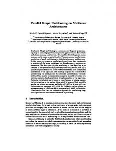
In this Section we focus on finding pargrp. algorithm/runtime t titions of the street networks of the DIBbest Bavg tavg [m] Kbest Kavg tavg [m] MACS Challenge. We implemented a lux. 79 79 60.1 81 83 0.1 specialized algorithm, Buffoon, which is bel. 307 307 60.5 320 326 0.9 similar to PUNCH [8] in the sense that net. 191 193 60.6 207 217 1.2 it also uses natural cuts as a preprocessita. 200 200 64.3 205 210 3.9 ing technique to obtain a coarser graph gb. 363 365 63.0 381 395 6.5 ger. 473 475 65.3 482 499 11.3 on which the graph partitioning problem asia. 47 47 67.6 52 55 6.4 is solved. For more information on natueur. 526 527 131.5 550 590 76.1 ral cuts, we refer the reader to [8]. Using our (shared memory) parallelized version Table 3. Results on road networks for k = 8: of natural cut preprocessing we obtain a average and best cut results of Buffoon (B) and coarse version of the graph. Note that our KaFFPa (K) as well as average runtime [m] (inpreprocessing uses slightly different pa- cluding preprocessing) . rameters than PUNCH (using the notan , f = 10, α = 1). Since partitions of the tion of [8], we use C = 2, U = (1 + ) 2k coarse graph correspond to partitions of the original graph, we use KaFFPaE to partition the coarse version of the graph. After preprocessing, we gave KaFFPaE one hour of time to compute a partition. In both cases we used all 16 cores (hyperthreading active) of machine C for preprocessing and for KaFFPaE. We also used the strong configuration of KaFFPa to partition the road networks. In both cases the experiments were repeated ten times. Table 3 summarizes the results.

7

Conclusion and Future Work

We presented two approaches to the graph partitioning problem, KaFFPa and KaFFPaE. KaFFPa uses novel local improvement methods and more sophisticated global search strategies to tackle the problem. KaFFPaE is an distributed evolutionary algorithm which uses KaFFPa as a base case partitioner. Due to new crossover and mutation operators as well as its scalable parallelization it is able to compute the best known partitions for many standard benchmark instances in only a few minutes. We therefore believe that KaFFPaE is still helpful in the area of high performance computing. Regarding future work, we want look at more DIMACS Instances, more values of k and more values of . In particular we want to have a closer look at the case  = 0. Furthermore we want to look at other objective functions such as communication volume.

References 1. R. Andersen and K.J. Lang. An algorithm for improving graph partitions. In Proceedings of the nineteenth annual ACM-SIAM symposium on Discrete algorithms, pages 651–660. Society for Industrial and Applied Mathematics, 2008. 2. Thomas B¨ack. Evolutionary algorithms in theory and practice : evolution strategies, evolutionary programming, genetic algorithms. PhD thesis, 1996.

14

3. David Bader, Henning Meyerhenke, Peter Sanders, and Dorothea Wagner. 10th DIMACS Implementation Challenge - Graph Partitioning and Graph Clustering, http://www.cc. gatech.edu/dimacs10/. 4. Una Benlic and Jin-Kao Hao. A multilevel memtetic approach for improving graph kpartitions. In 22nd Intl. Conf. Tools with Artificial Intelligence, pages 121–128, 2010. 5. Thang Nguyen Bui and Curt Jones. Finding good approximate vertex and edge partitions is NP-hard. Inf. Process. Lett., 42(3):153–159, 1992. 6. Pierre Chardaire, Musbah Barake, and Geoff P. McKeown. A probe-based heuristic for graph partitioning. IEEE Trans. Computers, 56(12):1707–1720, 2007. 7. Kenneth Alan De Jong. Evolutionary computation : a unified approach. MIT Press, 2006. 8. Daniel Delling, Andrew V. Goldberg, Ilya Razenshteyn, and Renato F. Werneck. Graph Partitioning with Natural Cuts. In 25th IPDPS. IEEE Computer Society, 2011. 9. Benjamin Doerr and Mahmoud Fouz. Asymptotically optimal randomized rumor spreading. In ICALP (2), volume 6756 of LNCS, pages 502–513. Springer, 2011. 10. D. Drake and S. Hougardy. A simple approximation algorithm for the weighted matching problem. Information Processing Letters, 85:211–213, 2003. 11. C. M. Fiduccia and R. M. Mattheyses. A Linear-Time Heuristic for Improving Network Partitions. In 19th Conference on Design Automation, pages 175–181, 1982. 12. P.O. Fjallstrom. Algorithms for graph partitioning: A survey. Linkoping Electronic Articles in Computer and Information Science, 3(10), 1998. 13. David E. Goldberg. Genetic algorithms in search, optimization, and machine learning. Addison-Wesley, 1989. 14. M. Holtgrewe, P. Sanders, and C. Schulz. Engineering a Scalable High Quality Graph Partitioner. 24th IEEE International Parallal and Distributed Processing Symposium, 2010. 15. G. Karypis, V. Kumar, Army High Performance Computing Research Center, and University of Minnesota. Parallel multilevel k-way partitioning scheme for irregular graphs. SIAM Review, 41(2):278–300, 1999. 16. Jin Kim, Inwook Hwang, Yong-Hyuk Kim, and Byung Ro Moon. Genetic approaches for graph partitioning: a survey. In GECCO, pages 473–480. ACM, 2011. 17. K. Lang and S. Rao. A flow-based method for improving the expansion or conductance of graph cuts. Integer Programming and Combinatorial Optimization, pages 383–400, 2004. 18. J. Maue and P. Sanders. Engineering algorithms for approximate weighted matching. In 6th Workshop on Exp. Alg. (WEA), volume 4525 of LNCS, pages 242–255. Springer, 2007. 19. Brad L. Miller and David E. Goldberg. Genetic algorithms, tournament selection, and the effects of noise. Complex Systems, 9:193–212, 1995. 20. V. Osipov and P. Sanders. n-Level Graph Partitioning. 18th European Symposium on Algorithms (see also arxiv preprint arXiv:1004.4024), 2010. 21. F. Pellegrini. Scotch home page. http://www.labri.fr/pelegrin/scotch. 22. P. Sanders and C. Schulz. Distributed Evolutionary Graph Partitioning (see ArXiv preprint arXiv:1110.0477). Technical report, Karlsruhe Institute of Technology, 2011. 23. P. Sanders and C. Schulz. Engineering Multilevel Graph Partitioning Algorithms. 19th European Symposium on Algorithms (see also arxiv preprint arXiv:1012.0006v3), 2011. 24. A.J. Soper, C. Walshaw, and M. Cross. A combined evol. search and multilevel optimisation approach to graph-partitioning. Journal of Global Optimization, 29(2):225–241, 2004. 25. C. Walshaw. Multilevel refinement for combinatorial optimisation problems. Annals of Operations Research, 131(1):325–372, 2004. 26. C. Walshaw and M. Cross. Mesh Partitioning: A Multilevel Balancing and Refinement Algorithm. SIAM Journal on Scientific Computing, 22(1):63–80, 2000. 27. C. Walshaw and M. Cross. JOSTLE: Parallel Multilevel Graph-Partitioning Software – An Overview. In F. Magoules, editor, Mesh Partitioning Techniques and Domain Decomposition Techniques, pages 27–58. Civil-Comp Ltd., 2007. (Invited chapter).

15

A

Detailed Walshaw Benchmark Results

Graph/k 2 4 8 16 32 64 add20 642 594 1 194 1 159 1 727 1 696 2 107 2 062 2 512 2 687 3 188 3 108 data 188 188 377 378 656 659 1 142 1 135 1 933 1 858 2 966 2 885 3elt 89 89 199 199 340 341 568 569 967 968 1 553 1 553 uk 19 19 40 40 80 82 144 146 251 256 417 419 add32 10 10 33 33 66 66 117 117 212 212 486 493 bcsstk33 10 096 10 097 21 390 21 508 34 174 34 178 55 327 54 763 78 199 77 964 109 811 108 467 whitaker3 126 126 380 380 654 655 1 091 1 091 1 678 1 697 2 532 2 552 crack 183 183 362 362 676 677 1 098 1 089 1 697 1 687 2 581 2 555 wing nodal 1 695 1 695 3 563 3 565 5 422 5 427 8 353 8 339 12 040 11 828 16 185 16 124 fe 4elt2 130 130 349 349 603 604 1 002 1 005 1 620 1 628 2 530 2 519 vibrobox 11 538 10 310 18 956 19 098 24 422 24 509 33 501 32 102 41 725 40 085 49 012 47 651 bcsstk29 2 818 2 818 8 029 8 029 13 904 13 950 22 618 21 768 35 654 34 841 57 712 57 031 4elt 138 138 320 320 532 533 932 934 1 551 1 547 2 574 2 579 fe sphere 386 386 766 766 1 152 1 152 1 709 1 709 2 494 2 488 3 599 3 584 cti 318 318 944 944 1 749 1 752 2 804 2 837 4 117 4 129 5 820 5 818 memplus 5 491 5 484 9 448 9 500 11 807 11 776 13 250 13 001 15 187 14 107 17 183 16 543 cs4 366 366 925 934 1 436 1 448 2 087 2 105 2 910 2 938 4 032 4 051 bcsstk30 6 335 6 335 16 596 16 622 34 577 34 604 70 945 70 604 116 128 113 788 176 099 172 929 bcsstk31 2 699 2 699 7 282 7 287 13 201 13 230 23 761 23 807 37 995 37 652 59 318 58 076 fe pwt 340 340 704 704 1 433 1 437 2 797 2 798 5 523 5 549 8 222 8 276 bcsstk32 4 667 4 667 9 195 9 208 20 204 20 323 35 936 36 399 61 533 60 776 94 523 91 863 fe body 262 262 598 598 1 026 1 048 1 714 1 779 2 796 2 935 4 825 4 879 t60k 75 75 208 208 454 454 805 815 1 320 1 352 2 079 2 123 wing 784 784 1 610 1 613 2 479 2 505 3 857 3 880 5 584 5 626 7 680 7 656 brack2 708 708 3 013 3 013 7 040 7 099 11 636 11 649 17 508 17 398 26 226 25 913 finan512 162 162 324 324 648 648 1 296 1 296 2 592 2 592 10 560 10 560 fe tooth 3 814 3 815 6 846 6 867 11 408 11 473 17 411 17 396 25 111 24 933 34 824 34 433 fe rotor 2 031 2 031 7 180 7 292 12 726 12 813 20 555 20 438 31 428 31 233 46 372 45 911 598a 2 388 2 388 7 948 7 952 15 956 15 924 25 741 25 789 39 423 38 627 57 497 56 179 fe ocean 387 387 1 816 1 824 4 091 4 134 7 846 7 771 12 711 12 811 20 301 19 989 144 6 478 6 478 15 152 15 140 25 273 25 279 37 896 38 212 56 550 56 868 79 198 80 406 wave 8 658 8 665 16 780 16 875 28 979 29 115 42 516 42 929 61 104 62 551 85 589 86 086 m14b 3 826 3 826 12 973 12 981 25 690 25 852 42 523 42 351 65 835 67 423 98 211 99 655 auto 9 949 9 954 26 614 26 649 45 557 45 470 77 097 77 005 121 032 121 608 172 167 174 482

Table 4. Computing partitions from scratch  = 1%. In each k-column the results computed by KaFFPaE are on the left and the current Walshaw cuts are presented on the right side.

16

Graph/k 2 4 8 16 32 64 add20 623 576 1 180 1 158 1 696 1 689 2 075 2 062 2 422 2 387 2 963 3 021 data 185 185 369 369 638 638 1 111 1 118 1 815 1 801 2 905 2 809 3elt 87 87 198 198 334 335 561 562 950 950 1 537 1 532 uk 18 18 39 39 78 78 140 141 240 245 406 411 add32 10 10 33 33 66 66 117 117 212 212 486 490 bcsstk33 10 064 10 064 20 767 20 854 34 068 34 078 54 772 54 455 77 549 77 353 108 645 107 011 whitaker3 126 126 378 378 650 651 1 084 1 086 1 662 1 673 2 498 2 499 crack 182 182 360 360 671 673 1 077 1 077 1 676 1 666 2 534 2 529 wing nodal 1 678 1 678 3 538 3 542 5 361 5 368 8 272 8 310 11 939 11 828 15 967 15 874 fe 4elt2 130 130 342 342 595 596 991 994 1 599 1 613 2 485 2 503 vibrobox 11 538 10 310 18 736 18 778 24 204 24 170 33 065 31 514 41 312 39 512 48 184 47 651 bcsstk29 2 818 2 818 7 971 7 983 13 717 13 816 22 000 21 410 34 535 34 400 55 544 55 302 4elt 137 137 319 319 522 523 906 908 1 523 1 524 2 543 2 565 fe sphere 384 384 764 764 1 152 1 152 1 698 1 704 2 474 2 471 3 552 3 530 cti 318 318 916 916 1 714 1 714 2 746 2 758 3 994 4 011 5 579 5 675 memplus 5 353 5 353 9 375 9 362 11 662 11 624 13 088 13 001 14 617 14 107 16 997 16 259 cs4 360 360 917 926 1 424 1 434 2 055 2 087 2 892 2 925 4 016 4 051 bcsstk30 6 251 6 251 16 399 16 497 34 137 34 275 69 592 69 763 113 888 113 788 173 290 171 727 bcsstk31 2 676 2 676 7 150 7 150 12 985 13 003 23 299 23 232 37 109 37 228 58 143 57 953 fe pwt 340 340 700 700 1 410 1 411 2 773 2 776 5 460 5 488 8 124 8 205 bcsstk32 4 667 4 667 8 725 8 733 19 956 19 962 35 140 35 486 59 716 58 966 91 544 91 715 fe body 262 262 598 598 1 018 1 016 1 708 1 734 2 738 2 810 4 643 4 799 t60k 71 71 203 203 449 449 793 802 1 304 1 333 2 039 2 098 wing 773 773 1 593 1 602 2 451 2 463 3 807 3 852 5 559 5 626 7 561 7 656 brack2 684 684 2 834 2 834 6 800 6 861 11 402 11 444 17 167 17 194 25 658 25 913 finan512 162 162 324 324 648 648 1 296 1 296 2 592 2 592 10 560 10 560 fe tooth 3 788 3 788 6 764 6 795 11 287 11 274 17 176 17 310 24 752 24 933 34 230 34 433 fe rotor 1 959 1 959 7 118 7 126 12 445 12 472 20 076 20 112 30 664 31 233 45 053 45 911 598a 2 367 2 367 7 816 7 838 15 613 15 722 25 563 25 686 38 346 38 627 56 153 56 179 fe ocean 311 311 1 693 1 696 3 920 3 921 7 657 7 631 12 437 12 539 19 521 19 989 144 6 434 6 438 15 203 15 078 25 092 25 109 37 730 37 762 55 941 56 356 78 636 78 559 wave 8 591 8 594 16 665 16 668 28 506 28 495 42 259 42 295 60 731 61 722 84 533 85 185 m14b 3 823 3 823 12 948 12 948 25 390 25 520 41 778 41 997 65 359 65 180 96 519 96 802 auto 9 673 9 683 25 789 25 836 44 785 44 832 75 719 75 778 119 157 120 086 170 989 171 535

Table 5. Computing partitions from scratch  = 3%. In each k-column the results computed by KaFFPaE are on the left and the current Walshaw cuts are presented on the right side.

17

Graph/k 2 4 8 16 32 64 add20 598 546 1 169 1 149 1 689 1 675 2 061 2 062 2 411 2 387 2 963 3 021 data 182 181 363 363 628 628 1 088 1 084 1 786 1 776 2 832 2 798 3elt 87 87 197 197 329 330 557 558 944 942 1 509 1 519 uk 18 18 39 39 75 76 137 139 237 242 395 400 add32 10 10 33 33 63 63 117 117 212 212 483 486 bcsstk33 9 914 9 914 20 167 20 179 33 919 33 922 54 333 54 296 77 457 77 101 106 903 106 827 whitaker3 126 126 377 378 644 644 1 073 1 079 1 650 1 667 2 477 2 498 crack 182 182 360 360 666 667 1 065 1 076 1 661 1 655 2 505 2 516 wing nodal 1 669 1 668 3 521 3 522 5 341 5 345 8 241 8 264 11 793 11 828 15 892 15 813 fe 4elt2 130 130 335 335 578 580 983 984 1 575 1 592 2 461 2 482 vibrobox 11 254 10 310 18 690 18 696 23 924 23 930 32 615 31 234 40 816 39 183 47 624 47 361 bcsstk29 2 818 2 818 7 925 7 936 13 540 13 575 21 459 20 924 33 851 33 817 55 029 54 895 4elt 137 137 315 315 515 515 888 895 1 504 1 516 2 514 2 546 fe sphere 384 384 762 762 1 152 1 152 1 681 1 683 2 434 2 465 3 528 3 522 cti 318 318 889 889 1 684 1 684 2 719 2 721 3 927 3 920 5 512 5 594 memplus 5 281 5 267 9 292 9 297 11 624 11 543 13 095 13 001 14 537 14 107 16 650 16 044 cs4 353 353 909 912 1 420 1 431 2 043 2 079 2 866 2 919 3 973 4 012 bcsstk30 6 251 6 251 16 189 16 186 34 071 34 146 69 337 69 288 112 159 113 321 170 321 170 591 bcsstk31 2 669 2 670 7 086 7 088 12 853 12 865 22 871 23 104 36 502 37 228 57 502 56 674 fe pwt 340 340 700 700 1 405 1 405 2 743 2 745 5 399 5 423 7 985 8 119 bcsstk32 4 622 4 622 8 441 8 441 19 411 19 601 34 481 35 014 58 395 58 966 90 586 89 897 fe body 262 262 588 588 1 013 1 014 1 684 1 697 2 696 2 787 4 512 4 642 t60k 65 65 195 195 443 445 788 796 1 299 1 329 2 021 2 089 wing 770 770 1 590 1 593 2 440 2 452 3 775 3 832 5 538 5 564 7 567 7 611 brack2 660 660 2 731 2 731 6 592 6 611 11 193 11 232 16 919 17 112 25 598 25 805 finan512 162 162 324 324 648 648 1 296 1 296 2 592 2 592 10 560 10 560 fe tooth 3 773 3 773 6 688 6 714 11 154 11 185 17 070 17 215 24 733 24 933 34 320 34 433 fe rotor 1 940 1 940 6 899 6 940 12 309 12 347 19 680 19 932 30 356 30 974 45 131 45 911 598a 2 336 2 336 7 728 7 735 15 414 15 483 25 450 25 533 38 476 38 550 56 377 56 179 fe ocean 311 311 1 686 1 686 3 893 3 902 7 385 7 412 12 211 12 362 19 400 19 727 144 6 357 6 359 15 004 14 982 25 030 24 767 37 419 37 122 55 460 55 984 77 430 78 069 wave 8 524 8 533 16 558 16 533 28 489 28 492 42 084 42 134 60 537 61 280 83 413 84 236 m14b 3 802 3 802 12 945 12 945 25 154 25 143 41 465 41 536 65 237 65 077 96 257 96 559 auto 9 450 9 450 25 271 25 301 44 206 44 346 74 636 74 561 119 294 119 111 169 835 171 329

Table 6. Computing partitions from scratch  = 5%. In each k-column the results computed by KaFFPaE are on the left and the current Walshaw cuts are presented on the right side.

18