May 28, 2015 - some of the other available free software for Bayesian inference on networks. .... conflict or double accounting with PC, the total prior is:.
arXiv:1505.07228v1 [stat.CO] 27 May 2015
Graph sampler : a C language software for fully Bayesian analyses of Bayesian networks Sagnik Datta* , Ghislaine Gayraud*,*** , Eric Leclerc* , and Frederic Y. Bois*,** *
Sorbonne universit´es, UTC ** INERIS *** Crest-Insee May 28, 2015 Abstract
Bayesian networks (BNs) are widely used graphical models usable to draw statistical inference about network structures. We present here Graph sampler a fast free C language software for structural inference on BNs. Graph sampler uses a fully Bayesian approach in which the marginal likelihood of the data (the data prior predictive distribution) and prior information about the network structure are considered. Inference on continuously valued BNs is treated as a Gaussian regression problem where the regressands are children nodes and the regressors their parents. Normal-gamma or Zellner likelihoods can then be used. For the discrete case a Dirichlet-multinomial model is available. A MetropolisHastings algorithm with fast jump kernel is used to sample graphs from their joint posterior distribution. The source C code distributed is very compact, fast, uses low memory and disk storage. We also reviewed the key features and working environment of other available software. As an illustration we compared the performance of our code to that of Structmcmc, a R package, using simulated data sets for graphs of 5 to 120 nodes. Our results show that Graph sampler is time efficient in identifying the underlying network and is time efficient. Several problems that arise when using Zellner priors are discussed. The relative weights of prior and likelihood are also discussed.
1
1
Introduction
Representing knowledge with uncertainty and automatic reasoning is often carried out using graphical models [1, 2, 3]. Judea Pearl and Richard E. Neapolitan were the first to summarize the properties of directed acyclic graphs (DAGs) and established them as a new field of study. In the recent years, formal statistical inference on systems of multiple interacting components is often done using DAGs [4] or Markov networks [5]. A Bayesian network (BNs) or a belief network is a probabilistic model denoted by a graph G = (V, E) in which each node or vertex v ∈ V represents one of the random variables in set X = (X1 , X2 , ..., XN ), where N is the number of nodes and each edge e ∈ E express the dependence among the variables in X. A BN is always directed and acyclic and is therefore a DAG. Besides static BNs, there are also dynamic BNs [6, 7], which are actually generalizations of hidden Markov models. In that paradigm, all the random variables of the network are considered to be potentially related to each other over adjacent time points. In computational biology and bioinformatics, BNs have been proposed, for example, for modeling gene regulatory networks, protein structure and gene expression. DAGs have been used for more than two decades in biomedicine and health-care for handling uncertainty in disease diagnosis, selecting the optimal treatment and predicting treatment outcome [8]. Other applications are found in social network analyses, high dimensional data analyses etc. Most of the available software programs which do BN parameter estimation or structural inference are generally slow and run on commercial platforms. Most of the results are presented for less than 30 nodes or so. Moreover many of them are not maintained regularly. In this article we present an efficient software for Bayesian inference on the structure of BN and perform a comparative study with Structmcmc, a versatile and easy to use R package [9]. The remainder of the paper is organized as follows: Section 2 briefly discusses the statistical inference for BNs with Graph sampler ; Section 3 is about the installation and running of Graph sampler ; Section 4 discusses the benmarking of Graph sampler for discrete as well as continuous data set along with the difficulties in the flipping technique and Section 5 presents some of the other available free software for Bayesian inference on networks. In Section 6 we discuss our results.
2
2
Statistical inference for BNs with Graph sampler
Recent work on BNs by Mukherjee and Speed [9], used Markov chain Monte Carlo (MCMC) simulations to infer on network structure from node values. They also considered priors encoding information relative to existence of edges, degree distribution and sparsity structure of the graph. Bois and Gayraud recently extended informative priors to account for motifs frequencies in order to generate realistic gene regulating graphs [10]. For baseline information they proposed to use Bernoulli distributions to model prior knowledge on individual edges. Variational Bayes (VB) methods have also been proposed as an alternative to full Bayesian inference. VB is an efficient way to deal with intractable integrals arising in a full Bayesian context and can be considered as an entension of the expectation-maximization (EM) algorithm [11]. VB can also help in model selection by providing a lower bound for the data marginal likelihood. However it provides only an approximate analytical solution for the posterior probability of the parameters and latent variables involved in a graphical model. Hence we focus here on a full Bayesian approach. The following sections describe the prior densities and data likelihood available in Graph sampler.
2.1
Priors on graph structure
It is quite a challenging problem to make inference on graphical model structure even with moderate number of variables, partly because of the huge number of possible graphs. For N nodes, the number of possible DAGs can be computed recursively [12] as: aN =
N X
k−1
(−1)
k=1
� � N k(N −k) 2 aN −k k
where a0 = 1 by convention. So for 2, 3, 4 and 5 node networks there are 3, 25, 543 and 29281 possible DAGs respectively. All of those possible graphs are usually not equally plausible a priori and thus certain features may be incorporated as more likely than the others, a priori. To make inference on graph structure, Bois and Gayraud [10] considered three different priors. In the most general case, a set of independent Bernoulli priors (PB ) is used to model the prior knowledge on individual edges. If pi,j is the probability of existence of a directed edge ei,j from node i to node j, and ei,j ∼ B(pi,j ) for all (i, j) ∈ {1, ..., N } × {1, ..., N }, then the
3
global Bernoulli prior PB on the graph G is PB (G) =
N Y
(pi,j )ei,j (1 − pi,j )1−ei,j
i6=j=1
The choice of the value for each hyperparameter pi,j depends on the prior evidence we have on the existence of the given edge from the scientific literature. The degree deg(v) of a vertex v is defined as the number of edges involving v. We can also define the degree distribution (PD ) for G as a function PD = card{v ∈ V : deg(v) = d} for all the vertices having degree d. The prior on degree can be expressed as a power law PD (G) ∝ d−γ ,
with
γ>0
In addition to PB and PD [9, 10], if we consider a Beta-Binomial prior (PM ) on the occurence of three-nodes motifs then the total prior on the graph G can be expressed in a product form as: PT (G) ∝ PB (G) × PD (G) × PM (G) Alternative to the Bernoulli prior for the presence of edges is the so called concordance prior (PC ) (see [9]). The latter required the specification of a prior matrix E with elements Ei,j = 1 representing a desired edge and -1 representing a non-desired edge. At each iteration the prior is calculated by counting the number of disagreements with the adjacency matrix A with elements Ai,j = 1 or 0 representing the presence or absence of edges between nodes i and j respectively of graph G. The form of the concordance prior is then PC (G) ∝ exp(−ρ|Ai,j − Ei,j |) where ρ is a positive valued hyperparameter. If PC is used, then the total prior is: PT (G) ∝ PC (G) × PD (G) × PM (G) or, equivalently, if PB is a flat prior (with pi,j = 0.5 for i 6= j) to avoid any conflict or double accounting with PC , the total prior is: PT (G) ∝ PB (G) × PC (G) × PD (G) × PM (G)
4
(1)
2.2
Data likelihood and the prior predictive distribution
Our main interest is to uncover the underlying structure of BNs. In any Bayesian network, a parent node has always an influence on its child nodes. Let us denote by x = (x1 , ..., xN ) the data we have on N nodes, where xi is a n-dimensional vector. Even though the model considered involves many parameters, the posterior distribution of each of these parameters are not of our primary interest. For computational reasons it is advisable to average out the parameters of f (·) analytically and to work with the prior predictive distribution [18]. Integrating out the parameters in Bayesian context is called Occam’s razor, since it allows simple explanations (models) for the given dataset over complex ones [19]. The prior predictive distribution or the joint N Q f (xi |Pa (xi )), marginal likelihood of the data can be expressed as f (x|G) = i=1
where Pa (xi ) is the set of parent values of xi in graph G [9] and f (·) is the prior predictive distribution of xi given its parenthood. For a global parent Pa (xi ) = ∅ and thus f (xi |Pa (xi )) reduces to f (xi ). 2.2.1
Case of a Gaussian regression model with a Normal-Gamma prior
The general expression for the linear Gausian regression for a given node xi is: xi = M (xi )β + u
(2)
where xi = (x1 , x2 , · · · , xn ) is a vector of n observations of the dependent variable x = ((xi,j )1≤i≤n;1≤j≤k ), k is the cardinality of Pa (xi ), M (xi ) is a so-called design matrix of order (n × k) with the first column as 1’s and other colums as Pa (xi ), β is a real valued vector of regression parameters of length k, and u follows a N (0, λ−1 In ) distribution with λ being a positive real valued precision and In is the identity matrix of order n. The likelihood for this regression model is therefore:
L(λ, β|xi , Pa (xi )) = (
λ λ n/2 ) exp(− (xi − M (xi )β)t (xi − M (xi )β)) 2π 2
where C t denotes the transpose of the matrix C. It is classical to choose conjugate form for the priors on the parameters
5
(i.e. β and λ) involved in the regression model : P (β, λ) = Nk (β | β0 , (n0 λ)−1 )Ga(λ | α, ω) � � k (ω)α (n0 )k/2 λ +α−1 t = (λ) 2 exp − (β − β0 ) n0 (β − β0 ) − ωλ (2π)k/2 Γ(α) 2 where β0 (real valued vector) and n0 (matrix of dimension k×k) are hyperparameters related to β and α, ω, both being real valued positive numbers, are hyper-parameters of λ. In the above equation Γ(.) represents the Gamma function. In that case, the prior predictive distribution is tν (µ, Σ), the n-dimensional multivariate t-distribution with parameters µ, Σ and ν, whose density function is: � �− ν+n 2 1 Γ(ν + n)/2 −1/2 t −1 1 + | Σ | (x − µ) Σ (x − µ) f (xi |Pa (xi )) = i i Γ(ν/2)(νπ)n/2 ν where, µ = [µ1 , . . . , µn ]t is the location parameter, Σ is the scalar matrix of dimension (k × k) and ν is the degrees of freedom and µ = Σ = h(M (xi )) = ν = −1
2.2.2
M (xi )β0 h(M (xi ))αω −1 In − M (xi )[M (xi )t M (xi ) + n0 ]−1 M (xi )t 2α
Case of a Gaussian regression model with a Zellner prior
With Graph sampler we can also use the Zellner g-prior [9, 21] for the parameters β and (λ)−1 : P (β|λ−1 ) = Nk (0, gλ−1 [M (xi )0 M (xi )]−1 ) and P (λ−1 ) ∝ λ where g is a user defined positive scale factor. The prior predictive distribution of the data is given by: f (xi |Pa (xi )) ∝ (1 + g)−(k+1)/2 s−n/2 where k is the cardinality of Pa (xi ) and g x0i M (xi )[M (xi )0 M (xi )]−1 M (xi )0 xi s = x0i xi − 1+g However, one of the disadvantage of the Zellner g-prior is that the number of parents for a dependent variable (child node) must be less than the number of observations for that variable (node). 6
2.2.3
Discrete data case
For discrete data, Graph sampler offers the possibility to use a Multinomial model with a Dirichlet prior on its parameters. In that case the closed form of the prior predictive [9] is given by: mi 0 0 Y Γ(Dijk + Dij ) ) Γ(Dij f (x|G) = · 0 Γ(Dij + Dij ) k=1 Γ(Dijk ) i=1 j=1 si n Y Y
where Dijk is the number of components of xi that takes the value k given 0 that Pa (xi ) has configuration j, Dijk are the Dirichlet hyperparameters, si represents the possible number of configurations of the parents of xi , mi 0 and Dij are given by: stands for the number of possible values of xi and Dij 0 Dij
=
mi X
0 Dijk
and
Dij =
k=1
2.3
mi X
Dijk
k=1
Efficient sampling of graphs
Graph sampler can efficiently generate random samples for general directed graphs [10], but we focus here on the sampling of BNs from a posterior distribution conditionned by data (observed node values). We use an adjacency matrix representation for the graph and store only the eventual difference between adjacency matrix as it is a fast and efficient storage method. A Metropolis-Hasting sampler [22] is used to sample random graphs according to the prescribed posterior probability distribution. If we denote the current graph by G and its adjacency matrix by AG , we first propose a new graph 0 G G0 through its adjacency matrix AG by selecting AG i,j while scanning A and then decide the presence of the edge ei,j by a random Bernoulli draw zi,j with probability pi,j (the Bernoulli prior for that edge). We use a simplified jumping kernel in which only adding or removing an edge is allowed. Thus while proposing G0 , if zi,j = 0, the proposed graph G0 is equal to G if AG i,j = 0, 0 G0 0 G else Ai,j is set to zero. For zi,j = 1, G will be equal G if Ai,j = 1, else AG i,j is set to one provided G0 is still a DAG. Scanning of the adjacency matrix is systematic (sweeping) as described in [10]. G0 is accepted with a probability f (x|G0 )PT (G0 )PB (G) ) δ = min(1, f (x|G)PB (G0 )PT (G) where x is the whole dataset, f (x|G) =
N Q
f (xi |Pa (xi )) is the prior predictive
i=1
and PT (·) is the total prior on the graph (·) structure. Clearly this simplifies 7
since PB (·) is a part of PT (·) (see eq(1)) In case of rejection, G’ is discarded, and the graph G remains the current graph. The procedure is repeated ˆ criterion until convergence in probability is attained. Gelman and Rubin’s R [24] is used on each element of the graph’s adjacency matrix to check the convergence of several simulation chains. For BNs we need to ensure that the proposed graphs are DAGs. This is done with a fast topological sorting algorithm (similar to that of [14]) operating on a list index of the nodes.
3
Graph sampler installation
Graph sampler is an easily available free software that can be redistributed or modified under the terms of the GNU General Public License as published by the Free Software Foundation. It is an inference as well as simulation tool for networks and can simulate random graphs for general directed graphs as well as for DAGs. In the case of BNs, we can also infer about their probable structure through the joint use of priors and data about node values. Graph sampler is written in ANSI-standard C language and can be compiled in any system having a ANSI C compliant compiler. The GNU gcc compiler (freeware) is highly recommended and the automated compilation script (called Makefile) can be successfully used if the standard ’make’ command is available. In order to modify the input file parser, the ’lex’ and ’yacc’ are highly recommended. The full software along with the manual can be downloaded from: https://sites.google.com/site/utcchairmmbsptp/software. Once downloaded, the software should be decompressed using ’gunzip’ and ’tar’ commands. Other archiving tools can also be used. Graph sampler can be compiled using the ’make’ command. On successful compilation of Graph sampler, it is ready for running. In order to run /textitGraph sampler, an input file specifying the simulation parameters should be provided. In Unix the command-line syntax to run that executable is: graph sampler [input-file [output-prefix]] where the brackets indicate optional arguments. If no input file and/or output prefix are not specified, the program uses the defaults. The default input file is script.txt and the output files created depends on the parameters specified in the input file. Default output file names are best graph.out, graph samples.out, degree count.out, motifs count.out edge p.out, results mcmc.bin. A Graph sampler input file is a text (ASCII) file that obeys relatively simple syntax (see the manual). Values of all the predefined variables in the input file should be properly defined. Description and range of each variable is illustrated in the manual. In case of improper assignment of 8
values, Graph sampler post error messages during runtime.
4
Graph sampler benchmarking
In order to benchmark the efficiency and accuracy of Graph sampler, an intensive comparison between Graph sampler and Structmcmc [9] was carried out. We selected the Structmcmc for comparison, because the sampling technique and the inference procedure of this software is very similar to Graph sampler and it helped us to explain the advantages and disadvantages efficiently. Structmcmc proposes a Zellner prior for continuous datasets and a Multivariate Dirichlet prior for discrete datasets. The Normal Gamma model is not available to Structmcmc users. In all the cases we used a null matrix as the initial adjacency matrix. For the prior on edges, we used the concordance prior [9] (PC ) with ρ = 1 since Structmcmc does not provide a Bernoulli prior. We followed the simulation procedure described in [9] to generate discrete datasets. For the continuous case, we generate data as described in equation (2). We simulated networks of 5 to 120 nodes, with 100 data points for each node. Figure 1 represents the network with 120 nodes. It is clearly a descending tree network. We used three different seeds to run three chains for each software program. We saved the three chains separately and calculated ˆ convergence diagnostic at each iteration. The first iteration for Gelman’s R ˆ which R attained at most 1.05 for all edges of the graph was considered as the minimum number of iterations required for convergence. Graph sampler was compiled with gcc version 4.2.1 (Apple Inc. build 5666) while Structmcmc was run with R 3.0.2 [33].
4.1
Discrete Case
We studied the performance of Graph sampler for discrete datasets, using the Multinomial model. Figure 2 gives a graphical summary of our timing results. Because of memory problems we could not achieve convergence with Structmcmc for networks of more than 60 nodes. Similarly for 120 nodes, Graph sampler did not converge with a billion iteration. Graph sampler was about 100 times faster than the Structmcmc for the same number of iterations. Graph sampler running time was also less influenced by the network size (i.e. it increased by a factor 4.06 when going from 5 to 60 nodes with Graph sampler and that factor being 16.5 for Structmcmc). With 30 nodes, Graph sampler took about 2 × 10⁷ iterations (275 seconds) to converge while for Structmcmc it was 106 iterations (3848 seconds). Thus Structmcmc re9
59 75
4
2
1
3
6
8
5
7
11
76
14 10 12
9
13 15 16
18 17 53
19 54 20 21
22 55
25 24 23 56 29 27 26 61 62 30 31 28 64 44 33 35 34 32 63 70 39 45
36
37 72 71
41 42 38 40 86 84 51
50
43 47
68
9 3 101
4 6 9 4 102
52 69 73
74
48 49
103 104
58 57 60
67
119 95 120
77
65 81 78 96
82
6 6 8 8 8 7 8 0 110
85 92 79 97 89 98 100 112 9 9 8 3 109 113 111
117
107
91 105
114 106
90 108
115
118 116
Figure 1: Hierarchical representation10 of the 120 nodes network used to generate our simulated data. All the other smaller networks were subsets from this network
quired 10 to 100 times less iterations to reach convergence but was about 14 times slower than Graph sampler . We compared the edge probability matrices from both the software by the accuracy curve to check whether they converge to the true graph.
B
Time (seconds)
1e+06 N=5 N = 10 N = 20 N = 30 N = 40 N = 60 N = 80 N = 100
1e+04
A 1e+02
1e+00 1e+03
1e+05
1e+07
1e+09
Number of iterations
Figure 2: Comparison of Graph sampler (A) and Structmcmc (B) performance for various network size (N) with discrete data. The x-axis represents the number of iterations performed and the y-axis the time taken on an Apple mac book 2.53 GHz Intel Core 2 Duo processor. The black lines with circles give the minimum number of iteration required to reach convergence. Figure 3 represents the posterior edge probabilities in the form of a heat map. It was observed that with small threshold values Structmcmc had higher accuracy than Graph sampler. Thus Structmcmc performed better than Graph sampler in retrieving edges correctly. However with a threshold values above 0.5, both the software had almost the same accuracy. Altogether, Graph sampler reaches convergence faster in time and has equal accuracy as Structmcmc for threshold values above 0.5.
11
�
�
�
�
Figure 3: Heat map of the true network with 30 nodes (A), heat map of the posterior edge probabilities obtained from Graph sampler with discrete data � and heat map of posterior edge probabilities obtained � (B) from Structmcmc with discrete data (C). The x-axis represent the parent nodes and the y-axis the corresponding children. The accuracy curve representing the efficiency of the two software for various threshold values (D). 4.1.1
Discrete case with degree prior
The accuracy of Graph sampler can be improved with the introduction of the degree prior (PD ) with γ = 2. As our network is a descending tree network, the inclusion of the degree prior is very beneficial. Figure 4(A) represents the posterior probabilities of the edges and resembles more like the true graph. It was observed that with the prior PD , the accuracy of Graph sampler improved significantly (figure 4(B)) and even with very low 12
threshold values, the accuracy was almost equal to 0.9. �
�
Figure 4: Heat map of the posterior edge probabilities obtained from Graph sampler with discrete data with concordance and degree priors (A) and the improvement in the accuracy curve due to the use of degree prior in Graph sampler (B). �
4.2
�
Continuous case
For continuous data, Structmcmc uses a Zellner prior on regression parameters. With Graph sampler either a normal-gamma prior or a Zellner prior can be used. The two models are compared here. 4.2.1
Graph sampler Normal-gamma model
For the continuous data set, convergence with Graph sampler was achieved with almost 10 times less iteration compared to Structmcmc. It was observed that with networks having 60 nodes, Structmcmc faced problems in convergence. Regarding the time taken for iterations, Graph sampler was almost 10 times faster than Structmcmc. For networks with more than 20 nodes, time efficiency of Structmcmc decreases sharply. The very narrow band width (A) reveals that for Graph sampler the increase in network size does not have much influence on time. Figure 5 represents our study in a graphical way. We also studied the posterior edge probabilities obtained from each of the software to draw inference on their efficiency to retrieve the true graph structure. We plotted the posterior edge probabilities in the form of heat 13
1e+06
Time (seconds)
B
N=5 N = 10 N = 20 N = 30 N = 40 N = 60 N = 80 N = 100 N = 120
1e+04
A
1e+02
1e+00 1e+05
1e+06
1e+07
1e+08
1e+09
Number of iterations
Figure 5: Comparison of Graph sampler (A) with the Structmcmc(B) for varying network size with continuous data set. The Graph sampler uses a normal gamma prior while Structmcmc uses a Zellner g-prior maps to compare the two software. Figure 6 represents the three heat maps for a network with 30 nodes. We plotted the accuracy curve for the two software. Figure 6(D) represents that the accuracy of Structmcmc is slightly higher than that of Graph sampler for smaller threshold values. However this difference is not much and for higher threshold values, both the software have almost equal accuracy. 4.2.2
Normal-gamma model with degree prior
The degree prior (PD ) with γ = 2 was introduced to check the improvement in the accuracy of Graph sampler. Figure 7(A) represents the posterior probabilities of the edges and resembles more like the true graph. It was observed that with the prior PD , there was no significant improvement in the accuracy of Graph sampler (figure 7(B)). 14
�
�
�
�
�
�
Figure 6: heat map of the true network with 30 nodes (A), heat map of the posterior edge probabilities estimated with Graph sampler (B), heat map for the Structmcmc code result (C). Here the x-axis represent the parents and y-axis the corresponding children and the accuracy curve for the two software (D). 4.2.3
Graph sampler Zellner model
For continuous datasets, we can also use the Zellner g-prior as used in Structmcmc. Unlike Structmcmc, we run Graph sampler for various g-prior values. We started with a g-prior of 1 for all the networks considered in our study. We checked the time required and the convergence point. Later we performed similar runs for different g-prior with values 5, 10, 50 and 100. In each case we observed the convergence rate and the posterior edge probabilities. 15
�
�
Figure 7: Heat map of the posterior edge probabilities obtained from Graph sampler with Normal-gamma model with concordance and degree priors (A) and the improvement in the accuracy curve due to the use of degree prior in Graph sampler (B). With a g-prior value of 1 or 5, convergence was achieved for all the networks. As we increased the value of g-prior to 10, runs with networks having � � ˆ being 1.12. This 5 and 10 nodes converged with the maximum value of R was not the case for networks with 20, 30, 40 and 60 nodes as they conˆ = 1.05 approx). However increasing the g-prior value to 50 and verged (R 100, convergence was not achieved for any of the networks. Thus in such a situation, Graph sampler and Structmcmc differs. For smaller network sizes, Graph sampler performed well with g-prior value equal to 1 or 5. With bigger networks sizes having 100 data points for each nodes, the g-prior value can range from 1 to 40. Graph sampler failed to converge when the g-prior value was equal to the number of data points. On the other hand, Structmcmc performed well with higher g-prior values and was most efficient when the g-prior value was equal to the number of data points. In order to understand the reason behind such a difference in convergence rate between the two software, we discuss the flipping technique used in Graph sampler along with its advantages and disadvantages. 4.2.4
Problem with flips
The primary advantage of the reduced jump kernel (only adding or deleting one edge at a time) used in Graph sapmpler is that it is faster than the jump kernel allowing flips. Since the choice of pairs of nodes is systematic, there 16
is no need to check the neighbourhood cardinality [6]. This jump kernel has some drawbacks also. Consider a network with 5 nodes where node 4 is a parent of node 5. In the MCMC simulations, at a particular step, we propose to add an edge from node 5 to node 4. As the log posterior for the proposed network is quite high (if 4 conditions 5, the two are correlated and 5 conditioning 4 has high probability), we accept such a proposal. According to our flipping technique, in order to retrieve the true edge (from 4 to 5), we need to first delete the edge from 5 to 4, leaving them independent. However a network with 4 and 5 independent has low log posterior probability and we rarely accept such a move. Figure 8 is a dot plot where the blue and the red dots appearing in pairs represents the difference in log probability for a network when passing from an edge (4 to 5) to an edge (5 to 4) respectively using the jump kernel specified in Graph sampler. For a pair A, a move from the red dot (log probability -675) to a blue dot (log probability -676), the log probability has to pass through -720 (4 and 5 independent) making such a move impossible. So in the most likely regions of G the flip is very unlikely. For the pair B, a move from the red dot (log probability of -698) to a state of independence (log probability of -685) is easy, but the next move to a blue dot (log probability of -700) is not easy. This is also an unlikely region where some flips are possible. The flip for the pair C is unlikely to occur as the log probability has to pass by -687 while going from -678 to -681. Flips would occur easily when they are close to the diagonal. The difficulty with the jump kernel can be due to the large data set for which the posterior mass favours fewer graphs. Under such a situation, the standard MCMC scheme faces difficulty in moving between graphs, or finding the high-scoring graphs. In such a case parallel tempering is a proficient option to speed up the MCMC-based convergence of network inference. This tempering approach is generally referred to as Model Composition by Metropolis-Coupled Markov Chain Monte Carlo (MC4 ) [28]. The parallel tempering involved in this MC4 approach allows proper mixing of the Markov chain and helps to escape the local maxima. 4.2.5
Sensitivity to the prior on graph structure
To check the sensitivity of the normal-gamma model with respect to informative and non informative priors, we considered a network with 40 nodes having 100 data points for each node and defined only the PB priors on the edges. We first considered an informative prior on edges with each desired edge having a prior probability of 0.9 and 0.1 for others except for autoloops for which probability was 0. We define a less informative prior with 0.8 and 17
-660
log probability of 5
A C
-680
B -700
-720
-740
-740
-720
-700
-680
-660
log probability of 4 independent of 5
Figure 8: The flips for a network with 5 nodes along with the log posterior probability after each flip. The blue dots represent the presence of the edge from 4 to 5 and the red dots for the edge from 5 to 4 in a 5 node network. The vertical and the horizontal lines in the graph are kept for easy reference of the marked pairs with both the axis. 0.2 and carry out our experimental run. We repeated the process and finally defined a flat non informative prior of 0.5 for all the edges. For each run with different prior probabilities, convergence was obtained in Graph sampler and then retrieved the posterior edge probabilities as it conveyed the information regarding the sensitivity of Graph sampler in selecting the desired graph out of all the equivalent graphs. With a strong informative prior of 0.9 and 0.1, Graph sampler converged and was able to retrieve all the desired edges with a high probability. The posterior probabilities of some undesired edges were also high. This is mainly observed as we move down the network due to the presence of partial correlation between the nodes higher up in the network and those at the bottom. As we use less informative priors, this behaviour becomes more prominent 18
and the efficiency of Graph sampler decreases (Figure 9). With a flat prior of 0.5 for all the edges, the efficiency of Graph sampler is the least. Figure 1 and the heat map of figure 9(A) show that the true network is a descending tree (the upper triangular matrix of the heat map has zero edge probability). For the informative prior, we observe that the normal-gamma model works well for the upper part of the tree network. However as we descend down the tree, the sensitivity of the model decreases as more children are involved. One way to increase the performance of the model can be by increasing the number of data points for each node present in the lower part of the network. We plotted the accuracy curve to depict the efficiency of Graph sampler for the various informative priors. Figure 9(D) represents the accuracy curve of Graph sampler. We observed that Graph sampler was very versatile with the type of prior information provided. With very strong prior the accuracy was almost equal to 0.9 for threshold values above 0.2. This stated that Graph sampler was efficient enough to retrieve the true edges with higher posterior probabilies and allot low probability (less than the threshold) to false edges. For noninformative priors Graph sampler had an accuracy of 0.65 for threshold below 0.3. The accuracy increased to 0.8 and above with the increase in threshold from 0.5 to 1.0. 4.2.6
Sensitivity to the degree prior on graph structure
We checked the sensitivity of Graph sampler for degree prior (PD ) with a noninformative Bernoulli prior on edges. We observed that there was not much improvement in the accuracy of Graph sampler in this case figure 10.
19
�
�
�
�
�
�
Figure 9: Heat map of the true (desired) network with 40 nodes (A), heat map of posterior edge probabilities obtained from Graph sampler with an informative prior of 0.9 for desired edges (B) and heat map of posterior edge probabilities obtained from Graph sampler with a noninformative prior of 0.5 (C) with a Normal gamma likelihood. Here the x-axis represent the parents and y-axis the corresponding children and the accuracy curve for the various informative priors (D) �
�
20 edge probabilities obtained from Figure 10: Heat map of the posterior Graph sampler with Normal-gamma model with a noninformative Bernoulli prior and degree priors (A) the accuracy curve due to the use of degree prior in Graph sampler (B). �
�
5
Other software
Apart from Structmcmc, there are several other very efficient BN software that are capable of performing Bayesian inference on parameter estimation and/or on network structure. Some of these software are free while others run on commercial platforms. Korb [23] presents some of the free software available presently that do inference on network structure. In this section we discuss about some of these software and their key features. B-Course: This is an online tool for data analysis allowing users to analyze data in the form of Bayesian networks. This tool is implemented as an Application Service Provider (ASP) and does not require any downloading or installation. B-Course requires a text file containing the user data in a tabular format. It has a good GUI and capable of doing inference on parameters as well as on network structure [29]. Banjo: This software was developed for structure learning of both static as well as Bayesian networks. This software lacks a proper GUI and the primary focus of this tool is on score-based structure inference. Banjo is uses the simulated annealing and greedy hill-climbing algorithm for inference. This software is written in Java and can do inference only on network structure. It is also good for dynamic Bayesian networks. BNT: This is a Matlab based software for inference on parameters and network structure. This software is suitable for both decision networks and dynamic Bayesian networks. However this tool lacks the GUI. Inference is carried out using various algorithms like the Junction tree, variable elimination and Pearl’s polytree. BNT has various options for parameter learning as well as for structure learning. It is very clearly documented, free and is very object-oriented. Elvira: This is tool is designed for constructing decision support systems based on models. This tool has a very good and easy GUI allowing users to define their respective models. Elvira is Java based and can be used in any operating system. This software is capable to doing inference on parameter estimation as well as on network structure. GMTk: This is an open source, readily available tool using dynamic graphical model (DGMs) and dynamic Bayesian networks (DBNs) for solving statistical models. This tool has a wide range of application in language processing, activity recognition, time series and in bioinformatics. GMTk allows both exact as well as approximate inference and includes dense, sparse and deterministic conditional probability tables. The GUI is very user friendly and inference can be carried out on both parameters and network structure. For the inference, this tool uses the junction tree algorithm. WinMine: This toolkit was developed for Windows 2000/NT/XP for 21
building statistical models from data. Most of the tools present here are command-line executable and requires very simple scripts. This tool is very well maintained and is updated periodically. This tool has a good GUI and can be used for both parameter estimation and inference on network structure. This tool cannot be used for commercial purpose. deal: This package is scripted in R language and uses BNs to analyse the data which can be discrete and/or continuous types. However this package is restricted to Gaussian networks. For the network parameters, suitable priors can be constructed and parameter estimation is possible using successive updating. This package is useful for structure learning of the network and uses the heuristic search algorithm [30]. statnet: This is also a R language software package for network analysis. This package uses the exponential-family random graph models (ERGM) for modelling of networks. This suite of packages includes several tools for effective model estimation, model-based network simulation, model evaluation and network visualization. statnet is based on MCMC algorithm that allows this package to deal with networks involving several thousand nodes. Moreover MCMC provides greater range, flexibility and insight into the network formation during network analysis. The coding of statnet is done in a combination of R and C language. Commands are generally provided from the command line from within the R graphical user interface. This suite of packages includes two obligatory tools and several user optional tools present in the Comprehensive R Archive Network (CRAN) [31]. Hadoop: This package is Java scripted and is very efficient for parameter as well as structure learning of continuous time BNs. This package uses the Gibbs sampling procedure. Structure learning is possible with both complete as well as incomplete data. Parameter learning is done for complete data using maximum likelihood and for incomplete data using expectation maximization algorithm. The learning algorithm for the continuous time BNs is the MapReduce algorithm. This package works well on a Linux OS, but is also efficient on Mac OS and Windows PC [32].
6
Discussion
We find that Graph sampler is efficient with respect to time and convergence. The Structmcmc is also a very efficient software coded in R language. However the time scaling with respect to N nodes inStructmcmc is not efficient. For large networks, Structmcmc faced problem in convergence. Graph sampler on the other hand is proficient in dealing with large networks and the time scaling is much lower compared to Structmcmc. The reduced 22
jump kernel proposed in Graph sampler makes it more faster and efficient compared to Structmcmc. This reduced jumping kernel requires less memory for storage. We observed that using Normal-gamma prior for the model parameters is better than the Zellner g-prior in uncovering the true edge probabilities. Disadvantage of using a Zellner g-prior is that number of parents should not be greater than the number of data points per node. Thus in actual situation where the number of parents is greater than number of available data, we cannot use the Zellner g-prior. Graph sampler has problems with convergence when using Zellner g-prior. Graph sampler is a very flexible software that allows to change the g-prior value accordingly. Focussing on time efficiency, convergence and retrievability of the desired network, Graph sampler is quite efficient and usable for large networks. Graph sampler is available in the following link: https://sites.google.com/site/utcchairmmbspt
7
Acknowledgments
S.D. is funded by a Ph.D. studentship for the French Ministry of Research.
23
References [1] Pearl, J. ”Probabilistic reasoning in intelligent systems: networks of plausible inference.”; San Mateo, CA, USA: Morgan Kaufmann; 1988. [2] Lauritzen, S.L. ”Graphical models.”; Oxford Univ Press, New York ; 1996. [3] Neapolitan, Richard E. ”Probabilistic reasoning in expert systems: theory and algorithms.”; Wiley. ISBN 978-0-471-61840-9.; 1990. [4] Heckerman, D., Geiger, D., and Chickering, D. ”Learning Bayesian Networks: The combination of Knowledge and Statistical Data.”; Machine Learning; vol. 20, pp 197-243, 1995. [5] Edwards, D.I. ”Introduction to graphical modelling.” ; 2nd ed. New York, USA: Springer ; 2000. [6] Husmeier, D. ”Sensitivity and specificity of inferring genetic regulatory interactions from microarray experiments with dynamic Bayesian networks.”; Bioinformatics; vol. 19, no. 17, pp 2271-2282, 2003. [7] Friedman, N., Murphy, K. and Russell, S. ”Learning the structure of dynamic probabilistic networks.” Proceedings of the Fourth Conference on Uncertainity in Artificial Intelligence (UAI) : Morgan Kaufmann Publishers Inc. San Francisco, CA, USA; pp 139-147, 1998. [8] Andreassen, S., Riekehr, C., Kristensen, B., Schonheyder, H.C., Leibovici, L. ”Using probabilistic and decision-theoretic methods in treatment and prognosis modeling.”; Artificial Intelligence in Medicine; vol 15, pp 121-134, 1999. [9] Mukherjee, S., and Speed, P. ” Network inference using informative priors.”; Proc Natl Acad Sci USA; vol. 105, no. 38 , pp 14313-14318 , September 2008. [10] Bois, F.Y. and Gayraud, G. ”Probabilistic generation of random networks taking into account information on motifs occurrence.”; Journal of Computational Biology; vol. 22, no. 1, pp 25-36, 2015. [11] Matthew, J. B. and Ghahramani, Z. ”The Variational Bayesian EM Algorithm for Incomplete Data: with Application to Scoring Graphical Model Structures.”; BAYESIAN STATISTICS 7 : Oxford University Press; editors: Bernardo, J.M., Bayarri, M.J., Berger, J.O., Dawid, A.P., Heckerman, D., Smith, A.F.M. and West M.; 2003. 24
[12] Robinson, R.W. ”Counting labeled acyclic digraphs.”; New Directions in the Theory of Graphs : New York Academic Press; pp 239-273, 1973. [13] Milo, R., Shen Orr S, Itzkovitz, S., Kashtan, N., Chklovskii, D., Alon, U. ” Network Motifs: Simple Building Blocks of Complex Networks.”; Science; vol. 298, pp 824-827, 2002. [14] Pearce, D.J. and Kelly, P.H.J. ”A dynamic topological sort algorithm for directed acyclic graphs.”; ACM Journal of Experimental Algorithmics; vol. 11, pp 1-7, 2006. [15] Alon, U. ” Network motifs: theory and experimental approaches.”; Nature Reviews Genetics; vol. 8, pp 450-461, 2007 [16] Shen Orr S, Milo, R., Mangan, S. and Alon, U. ” Network Motifs in the transcriptional regulation network of Escherichia coli.”; Nat. Ganet.; vol. 31, pp 64-68, 2002. [17] Mangan, S., Zaslaver, A. and Alon, U. ”The coherent feedforward loop serves as a sign-sensitive delay element in transcription networks. ”; J. Mol. Biol.; vol. 334, pp 197-204, 2003. [18] Ickstadt,K. ”Nonparametric Bayesian Networks (with discussion.”; In Bernardo,J. et al. (ed.)Bayesian Statistics 9. Oxford University Press, Oxford ; pp. 135–155, 2010. [19] Jefferys, W.H. and Berger, J.O. ”Ockham’s razor and Bayesian analysis”; American Scientist; vol 80, pp 64-72 , 1992. [20] Beal. ”Variational algorithms for approximate Bayesian Inference.”; PhD. thesis; 1998. [21] Nott, D.J. and Green, P.J. ”Bayesian Variable Selection and the Swendsen- Wang Algorithm.”; Journal of Computational and Graphical Statistics; vol. 13, no. 1, 2004. [22] Casella, G. and Robert, C.P. ”Monte Carlo Statistical Methods.”; Springer-Verlag , Berlin; 2004. [23] Korb, K.B. and Nicholson, A.E. ”Bayesian Artificial Intelligence.”; CRC Press, editors: David Blei, Princeton University, David Madigan, Rutgers University, Marina Meila, University of Washington and Fionn Murtagh, Royal Holloway, University of London; pp 414-415, 2010.
25
[24] Gelman, A. and Rubin, D.B. ”Inference from iterative simulation using multiple sequences.”; Stat. Sci.; vol 7, pp 457-511, 1992. [25] Murphy, K. ”Software for Graphical Models : A Review.”; ISBA (Intl. Soc. for Bayesian Analysis) Bulletin; vol. 14, no. 4, pp 13-15, 2007. [26] Celeux, G., Anbari, M.El., Marin, J.M. and Robert, C.P. ”Regularization in regression: comparing Bayesian and frequentist methods in a poorly informative situation.”; Bayesian Anal.; vol. 2, pp 477-502, 2012. [27] Kass R. and Wasserman L. ”A reference Bayesian test for nested hypotheses and its relationship to the Schwarz criterion.”; J. American Statist. Assoc.; vol. 90, pp 928-934, 1995. [28] Barker, D.J., Hill, S.M. and Mukherjee, S. ”MC4: A Tempering Algorithm for Large-Sample Network Inference.”; Pattern Recognition in Bioinformatics; vol. 6282, pp 431-442, 2010. [29] Myllymaki, P., Silander, T., Tirri, H. and Uronen, P. ”B-COURSE: A web-based tool for Bayesian and causal data analysis.”; Int. J. Artif. Intell. Tools; vol. 11, no. 3, 2002. [30] Boettcher, S.G. and Dethlefsen, C. ”deal: A Package for Learning Bayesian Networks.”; Journal of Statistical Software; vol. 8, no. 20, 2003. [31] Handcock, M.S., Hunter, D.R., Butts, C.T., Goodreau, S.M. and Morris, M. ”statnet: Software Tools for the Representation, Visualization, Analysis and Simulation of Network Data.”; Journal of Statistical Software; vol. 24, no. 1, 2008. [32] Villa, S. and Rossetti, M. ”Learning Continuous Time Bayesian Network Classi ers Using MapReduce.”; Journal of Statistical Software; vol. 62, no. 3, 2014. [33] R Core Team ”R: A Language and Environment for Statistical Computing.”; R Foundation for Statistical Computing, Vienna, Austria; http://www.R-project.org/, 2013.
26