to the NETWORK dataset in our experiments; (b) Email net- .... Parameter-free: GraphScope is completely automatic, requiring no ...... We construct sender-to-.
Research Track Paper
GraphScope: Parameter-free Mining of Large Time-evolving Graphs Jimeng Sun‡ Philip S. Yu§ ‡
Spiros Papadimitriou§ Christos Faloutsos‡
Carnegie Mellon University
§
IBM TJ Watson lab
{spapadim,psyu}@us.ibm.com
{jimeng,christos}@cs.cmu.edu
ABSTRACT
To complicate matters further, large amounts of data such as those in the above examples are continuously collected and patterns are also changing over time. Therefore, batch methods for pattern discovery are not sufficient. We need tools that can incrementally find the communities and monitor the changes. In summary, there are two key problems that need to be addressed:
How can we find communities in dynamic networks of social interactions, such as who calls whom, who emails whom, or who sells to whom? How can we spot discontinuity timepoints in such streams of graphs, in an on-line, any-time fashion? We propose GraphScope, that addresses both problems, using information theoretic principles. Contrary to the majority of earlier methods, it needs no user-defined parameters. Moreover, it is designed to operate on large graphs, in a streaming fashion. We demonstrate the efficiency and effectiveness of our GraphScope on real datasets from several diverse domains. In all cases it produces meaningful time-evolving patterns that agree with human intuition.
P1) Community discovery: Which groups or communities of nodes are associated with each other? P2) Change detection: When does the community structure change and how to quantify the change? Moreover, we want to answer these questions (a) without requiring any user-defined parameters, and (b) in a streaming fashion. For example, we want to answer questions such as: How do the network hosts interact with each other? What kind of host groups are there, e.g., inactive/active hosts; servers; scanners? Who emails whom? Do the email communities in a organization such as ENRON remain stable, or do they change between workdays (e.g., business-related) and weekends (e.g., friend and relatives), or during major events (e.g.,the FBI investigation and CEO resignation)? We propose GraphScope, which addresses both of the above problems simultaneously. More specifically, GraphScope is an efficient, adaptive mining scheme on time-evolving graphs. Unlike many existing techniques, it requires no userdefined parameters, and it operates completely automatically, based on the Minimum Description Length (MDL) principle. Furthermore, it adapts to the dynamic environment by automatically finding the communities and determining good change-points in time. In this paper we consider bipartite graphs, which treat source and destination nodes separately (see example in Figure 2). As will become clear later, we discover separate source and destination partitions, which are desirable in several application domains. Nonetheless, our methods can be easily modified to deal with unipartite graphs, by constraining the source-partitions to be the same as the destinationpartitions [6]. The main insight of dealing with such graphs is to group “similar” sources together into source-groups (or row-groups), and also “similar” destinations together, into destinationgroups (or column-groups). Examples in Section 6.2 show how much more orderly (and easier to compress) the adjacency matrix of a graph is, after we strategically re-order its rows and columns. The exact definition of “similar” is actually simple, and rigorous: the most similar source-partitions
Categories and Subject Descriptors H.2.8 [Database applications]: Data mining
General Terms Algorithms
1. INTRODUCTION Graphs arise naturally in a wide range of disciplines and application domains, since they capture the general notion of an association between two entities. However, the aspect of time has only recently begun to receive some attention [15, 20]. Some examples of the time-evolving graphs include: (a) Network traffic events indicate ongoing communication between source and destination hosts, similar to the NETWORK dataset in our experiments; (b) Email networks associate a sender and a recipient at a given date, like the ENRON data set [2] in the experiments; (c) Call detail records in telecommunications networks associate a caller with a callee. The set of all conversation pairs over each week forms a graph that evolves over time, like the publicly available ‘CELLPHONE’ dataset of MIT users calling each other [1]; (d) Transaction data: in a financial institution, who accessed what account, and when; (e) In a database compliance setting [4], again we need to record which user accessed what data item and when.
Permission to make digital or hard copies of all or part of this work for personal or classroom use is granted without fee provided that copies are not made or distributed for profit or commercial advantage and that copies bear this notice and the full citation on the first page. To copy otherwise, to republish, to post on servers or to redistribute to lists, requires prior specific permission and/or a fee. KDD’07, August 12–15, 2007, San Jose, California, USA. Copyright 2007 ACM 978-1-59593-609-7/07/0008 ...$5.00.
687
Research Track Paper
2. RELATED WORK
for a given source node is the one that leads to small encoding cost (see Section 4 for more details). Furthermore, if these communities (source and destination partitions) do not change much over time, consecutive snapshots of the evolving graphs have similar descriptions and can also be grouped together into a time segment, to achieve better compression. Whenever a new graph snapshot cannot fit well into the old segment (in terms of compression), GraphScope introduces a change-point, and starts a new segment at that time-stamp. Those change points often detect drastic discontinuities in time. For example on the ENRON dataset, the change points all coincide with important events related to the ENRON company, as shown in Figure 1 (more details in Section 6.2).
Here we discuss related work from three areas: mining static graphs, mining dynamic graphs, and stream mining.
2.1 Static Graphs Graph mining has been a very active area in the data mining community. From the exploratory aspect, Faloutsos et al. [10] have shown the power-law distribution on the Internet graph. Kumar et al. [14] discovered the bow-tie model for web graphs. From the algorithmic aspect, graph partitioning has attracted much interest, with prevailing methods being METIS [12] and spectral partitioning [16]. Even in these topperforming methods, users must specify the number of partitions k. Moreover, they typically also require a measure of imbalance between the two pieces of each cut. Information-theoretic Co-clustering [9] simultaneously reorders the rows and columns of a normalized contingency table or a two-dimensional probability distribution, where the number of clusters has to be specified. The Cross-association method [7] formulates the co-clustering problem as a binary matrix compression problem. Noble and Cook [17] propose an entropy-based anomaly detection scheme for graphs. All these methods deal with static matrices or graphs, while GraphScope is designed to work with dynamic streams. Moreover, most of methods except for cross-association require some user-defined parameters, which may be difficult to set and which may dramatically affect the final result, as observed in [13]. Keogh et al. [13] proposed the notion of parameter free data mining. GraphScope shares the same spirit but focuses on different problems. In addition to graph mining, several storage schemes [11, 18] have been proposed to compress large binary matrices (graphs) by column reordering. However, none of those scheme perform both column and row reordering and their focus is on compression rather than mining.
Enron timeline
15K
Intensity
Cost savings (split)
20K
10K 5K 0 −5K 0
20
40 60 80 100 Nov 1999: Enron launched
120
140
160
Feb 2001: Jeffrey Skilling takes over as CEO Jun 2001: Rove divests his stocks in energy 14 Aug 2001: Kenneth Lay takes over as CEO 19 Nov 2001: Enron restates 3rd quarter earnings 29 Nov 2001: Dynegy deal collapses 10 Jan 2002: DOJ confirms criminal investigation begun 23 Jan 2002: Kenneth Lay resigns from CEO 23 Jan 2002: FBI begins investigation of document shredding 30 Jan 2002: Enron names Stephen F. Cooper new CEO 4 Feb 2002: Lay implicated in plot to inflate profits and hide losses 24 Apr 2002: House passes accounting reform package
Figure 1: ENRON dataset (Best viewed in color). Relative compression cost versus time. Large cost indicates change points, which coincide with the key events. E.g., at time-tick 140 (Feb 2002), CEO Ken Lay was implicated in fraud.
2.2 Dynamic Graphs From the exploratory viewpoint, Leskovec et al. [15] discovered the shrinking diameter phenomena on time-evolving graphs. Backstrom et al. [5] study community evolution in social networks. From the algorithmic aspect, Sun et al. [20] present dynamic tensor analysis, which incrementally summarizes tensor streams (high-order graph streams) as smaller core tensor streams and projection matrices. This method still requires user-defined parameters (like the size of the core tensor). Moreover, it gives lossy compression. Aggarwal and Yu [3] propose a method to selectively store a subset of graphs to approximate the entire graph stream and to find community changes in time-evolving graphs based on the user specified time interval and the number of communities. Again, our GraphScope framework avoids all these user-defined parameters.
Contributions. Our proposed approach, GraphScope, monitors communities and their changes in a stream of graphs efficiently. It has the following key properties: • Parameter-free: GraphScope is completely automatic, requiring no parameters from the user (like number of communities, thresholds to assess community drifts, and so on). Instead, it is based on sound informationtheoretic principles, specifically, MDL. • Adaptive: It can effectively track communities over time, discovering both communities as well as changepoints in time, that agree with human intuition. • Streaming: It is fast, incremental and scalable for the streaming environment. We demonstrate the efficiency and effectiveness of our approach in discovering and tracking communities in real graphs from several domains.
3. PROBLEM DEFINITION In this section, we formally introduce neccessary notation and formulate the problems.
The rest of the paper is organized as follows: Section 2 reviews the related work. Section 3 introduces some necessary definitions and formalizes the problem. Section 4 presents the objective function. Section 5 presents our proposed method to search for an optimal solution, Section 6 shows the experimental evaluation and Section 7 concludes.
3.1 Notation and definition Calligraphic letters always denote graph streams or graph stream segments (consisting of one or more graph snapshots),
688
Research Track Paper Sym. G, G (s) t m, n G(t) i, j (t) Gi,j s ts ks ,!s p, q (s) Ip (s)
Jq (s) mp (s) np (s) Gp,q (s) |Gp,q | (s)
|E|p,q (s) ρp,q
H(.)
Definition Graph stream, Graph segment Timestamp, t ≥ 1. Number of source(destination) nodes. Graph at time t (m × n adjacency matrix). Node indices, 1 ≤ i ≤ m, 1 ≤ j ≤ n. Indicator for edge (i, j) at time t. Graph segment index, s ≥ 1. Starting time of s-th segment. Number of source (dest.) partitions for segment s. Partition indices, 1 ≤ p ≤ ks , 1 ≤ q ≤ !s . Set of sources belonging to the p-th partition, during the s-th segment. (s) Similar to Ip , but for destination nodes. (s) (s) Source partition size, mp ≡ |Ip |, 1 ≤ p ≤ ks . (s) (s) Dest. partition size, np ≡ |Jp |, 1 ≤ p ≤ !s . Subgraphs induced by p-th and q-th partitions of segment s, i.e., subgraph segment (s) (s) (s) Size of subgraphs segment, |Gp,q | := mp nq (ts+1 − ts ). (s) Number of edges in Gp,q (s)
Density of Gp,q ,
Intuitively, a “graph stream segment” (or just “graph segment”) is a set of consecutive graphs in a graph stream. For example in Figure 2, G (1) is a graph segment consisting of two graph G(1) and G(2) . Next, within each segment, we will partition the source and destination nodes into source partitions and destination partitions, respectively. Definition 3.3 (Graph segment partitions). For each segment s ≥ 1, we partition source nodes into ks source partitions and destination nodes into !s destination partitions. The set of source nodes that are assigned into the p(s) th source partition 1 ≤ p ≤ ks is denoted by Ip . Similarly, the set of destination nodes assigned to the q-th destination (s) partition is denoted by Jq , for 1 ≤ q ≤ !s . (s)
The sets Ip (1 ≤ p ≤ ks ) partition the source nodes, in the S (s) (s) (s) sense that Ip ∩Ip! = ∅ for p (= p" , while p Ip = {1, . . . , m}. (s)
Similarly, the sets Jq (1 ≤ q ≤ ls ) partition the destination nodes. For example in Figure 2, the first graph segment (1) (1) G (1) has source partitions I1 = {1, 2}, I2 = {3, 4}, and (1) (1) destination partitions J1 = {1}, J2 = {2, 3} where k1 = 2, !1 = 2. We can similarly define source and destination partition for the second graph segment G (2) , where k2 = 3, !2 = 3.
(s)
|E|p,q
(s) |Gp,q |
Shannon entropy function
3.2 Problem formulation
Table 1: Definitions of symbols while individual graph snapshots are denoted by non-calligraphic, upper-case letters. Superscripts in parentheses denote either timestamps t or graph segment indices s, accordingly. Similarly, subscripts denote either individual nodes i, j or node partitions p, q.
In this paper, the ultimate goals are to find communities on time-evolving graphs along with the change-points, if any. Thus, the following two problems need to be addressed. Problem 1 (Partition Identification). Given a graph stream segment G (s) , how to find good partitions of source and destination nodes, which summarize the fundamental community structure.
Definition 3.1 (Graph stream). A graph stream G is a sequence of graphs G(t) , i.e., G := {G(1) , G(2) , . . . , G(t) , . . .},
The meaning of “good” will be made precise in the next section, which formulates our cost objective function. However, to obtain an answer for the above problem, two important sub-questions need to be answered (see Section 5.1):
which grows indefinitely over time. Each of these graphs links m source nodes to n destination nodes. For example in Figure 2, the first row shows the first three graphs in a graph stream, where m = 4 and n = 3. Furthermore, the graphs are represented as sparse matrices in the bottom of Figure 2 (a black entry is 1, which indicates an edge between the corresponding nodes; likewise a white entry is 0). In general, each graph may be viewed as an m × n binary adjacency matrix, where rows 1 ≤ i ≤ m correspond to source nodes and columns 1 ≤ j ≤ n correspond to destination nodes. We use sparse representation of the matrix (i.e., only non-zero entries are stored) whose space consumption is similar to adjacency list representation. Without loss of generality, we assume m and n are the same for all graphs in the stream; if not, we can introduce all-zero rows or columns in the adjacency matrices. One of our goals is to track how the structure of the graphs G(t) , t ≥ 1, evolves over time. To that end, we will group consecutive timestamps into segments.
• How to assign the m source and n destination nodes into ks source and !s destination partitions? • How to determine ks and !s ? Problem 2 (Time Segmentation). Given a graph stream G, how can we incrementally construct graph segments, by selecting good change points ts . Section 5.2 presents the algorithms and formalizes the notion of “good” for both problems above. We name the whole analytic process GraphScope.
4. GRAPHSCOPE ENCODING OBJECTIVE Our mining framework is based on one form of the Minimum Description Length (MDL) principle and employs a lossless encoding scheme for a graph stream. Our objective function estimates the number of bits needed to encode the full graph stream so far. Our proposed encoding scheme takes into account both the community structures, as well as their change points in time, in order to achieve a concise description of the data. The fundamental trade-off that decides the “best” answers to problems 1 and 2 in Section 3.2
Definition 3.2 (Graph stream segment). The set of graphs between timestamps ts and ts+1 −1 (inclusive) consist the s-th segment G (s) , s ≥ 1, which has length ts+1 − ts , G (s) := {G(ts) , G(ts +1) , . . . , G(ts+1 −1) }.
689
Research Track Paper cost for storing three integers is log!|E| + log!m + log!n bits, where log!is the universal code length for an integer2 . Notice that this scheme can be extended to a sequence of graphs in a segment. More generally, if the random variable X can take values from the set M , with size |M | (a multinomial distribution), the entropy of X is P H(X) = − x∈M p(x) log p(x).
where p(x) is the probability that X = x. Moreover, the 1 for all x ∈ M maximum of H(X) is log |M | when p(x) = |M | (pure random, most difficult to compress); the minimum is 0 when p(x) = 1 for a particular x ∈ M (deterministic and constant, easiest to compress). For the binomial case, if all symbols are all 0 or all 1 in the string, we do not have to store anything because by knowing the number of ones in the string and the sizes of matrix, the receiver is already able to decode the data completely. With this observation in mind, the goal is to organize the matrix (graph) into some homogeneous sub-matrices with low entropy and compress them separately, as we will describe next.
Figure 2: Notation illustration: A graph stream with 3 graphs in 2 segments. First graph segment consisting (1) of G(1) and G(2) has two source partitions I1 = {1, 2}, (1)
(1)
(1)
I2 = {3, 4}; two destination partitions J1 = {1}, J2 = {2, 3}. Second graph segment consisting of G(3) has three (2) (2) (2) source partitions I1 = {1}, I2 = {2, 3}, I3 = {4}; three (2)
(2)
4.2 Graph Segment encoding
(2)
destination partitions J1 = {1}, J2 = {2}, J2 = {3}.
Given a graph stream segment G (s) and its partition assignments, we can precisely compute the cost for transmitting the segment as two parts: 1) Partition encoding cost: the model complexity for partition assignments, 2) Graph encoding cost: the actual code for the graph segment.
is between (i) the number of bits needed to describe the communities (or, partitions) and their change points (or, segments) and (ii) the number of bits needed to describe the individual edges in the stream, given this information. We begin by first assuming that the change-points as well the source and destination partitions for each graph segment are given, and we show how to estimate the bit cost to describe the individual edges (part (ii) above). Next, we show how to incorporate the partitions and segments into an encoding of the entire stream (part (i) above).
4.1
Partition encoding cost The description complexity for transmitting the partition assignments for graph segment G (s) consists of the following terms: First, we need to send the number of source and destination nodes m and n using log!m + log!n bits. Note that, this term is constant, which has no effect on the choice of final partitions. Second, we shall send the number of source and destination partitions which is log!ks + log!!s . Third, we shall send the source and destination partition assignments. To exploit the non-uniformity across partitions, the encoding cost is mH(P ) + nH(Q) where P is a
Graph encoding
In this paper, a graph is presented as a m-by-n binary matrix. For example in Figure 2, G(1) is represented as 0 1 1 0 0 B 1 0 0 C C G(1) = B (1) @ 0 1 1 A 0 0 1
(s)
m
Conceptually, we can store a given binary matrix as a binary string with length mn, along with the two integers m and n. For example, equation 1 can be stored as 1100 0010 0011 (in column major order), along with two integers 4 and 3. To further save space, we can adopt some standard lossless compression scheme (such as Huffman coding, or arithmetic coding [8]) to encode the binary string, which formally can be viewed as a sequence of realizations of a binomial random variable X. The code length for that is accurately estimated as mnH(X) where H(X) is the entropy of variable X. For notational convenience, we also write that as mnH(G(t) ). Additionally, three integers need to be stored: the matrix sizes m and n, and the number of ones in the matrix (i.e., the number of edges in the graph) denoted as |E| 1 . The 1
|E| is needed for computing the probability of ones or zeros, which is required for several encoding scheme such as Huffman coding
690
multinomial random variable with the probability pi = mi (s) and mi is the size of i-th source partition 1 ≤ i ≤ ks ). Similarly, Q is another multinomial random variable with (s)
n
(s)
qi = ni and ni is the size of i-th destination partition, 1 ≤ i ≤ !s . For example in Figure 2, the partition sizes for first seg(1) (1) (1) (1) ment G (1) are m1 = m2 = 2, n1 = 1, and n2 = 2; the (1) 2 2 partition assignments for G costs −4( 4 log( 4 )+ 24 log( 24 ))− 3( 13 log( 13 ) + 32 log( 32 )) bits. In summary, the partition encoding cost for graph segment G (s) is Cp(s)
:=
log!m + log!n + log!ks + log!!s +
(2)
mH(P ) + nH(Q) 2
To encode a positive integer x, we need log!x ≈ log2 x + log2 log2 x + . . ., where only the positive terms are retained and this is the optimal length, if the range of x is unknown [19]
Research Track Paper where P and Q are multinomial random variables for source and destination partitions, respectively.
Having defined the objective precisely in equation 3 and equation 4, the next step is to search for optimal partition and time segmentation. However, finding the optimal solution is NP-hard3 . Next, in Section 5, we present an alternating minimization method coupled with an incremental segmentation process to perform the overall search.
Graph encoding cost After transmitting the partition encoding, the actual graph segment G (s) is transmitted as ks !s subgraph segments. To facilitate the discussion, we define the entropy term for a (s) subgraph segment Gp,q as ` (s) (s) (s) (s) (s) ´ H(Gp,q ) = − ρp,q log ρp,q + (1 − ρp,q ) log(1 − ρp,q ) (3) (s)
(s)
where ρp,q =
|E|p,q
(s) |Gp,q |
(s)
5. GRAPHSCOPE In this section we describe our method, GraphScope by solving the two problems proposed in Section 3.2. The goal is to find the appropriate number and position of changepoints, and the number and membership of source and destination partitions so that the cost of (6) is minimized. Exhaustive enumeration is prohibitive, and thus we resort to alternating minimization. Note that we drop the subscript s on ks and !s whenever it is clear from the context. Specifically, we have two steps: (a) how to find good communities (source and destination partitions), for a given set of graph snapshots that belong to the same segment. (b) when to declare a time-tick as a change point and start a new graph segment. We describe each next.
(s)
is the density of subgraph segment Gp,q .
Intuitively, H(Gp,q ) quantifies how difficult it is to compress (s) the subgraph segment Gp,q . In particular, if the entire subgraph segment is all 0 or all 1 (the density is exactly 0 or 1), the entropy term becomes 0. With this, the graph encoding cost is Cg(s) :=
ks X "s X ` p=1 q=1
(s)
(s) (s) (s) ´ log!|E|p,q + |Gp,q | · H(Gp,q ) .
(4)
5.1 Partition Identification
where |E|p,q is the number of edges in the (p, q) sub-graphs (s) of segment s; |Gp,q | is the size of sub-graph segment, i.e, (s) (s) (s) mp nq (ts+1 −ts ), and H(Gp,q ) is the entropy of the subgraph segment defined in equation 3. (1) In the sub-graph segment G2,2 of Figure 2, the number (1)
Here we explain how to find source and destination partitions for a given graph segment G (s) . In order to do that, we need to answer the following two questions: • How to find the best partitioning given the number of source and destination partitions?
(1)
(1)
of edges |E|2,2 = 3 + 4, G2,2 has the size |G2,2 | = 2 × 2 × 2, (1)
(1)
the density ρ2,2 = 87 , and the entropy H(G2,2 ) = −( 78 log 87 + 1 log 18 ). 8 Putting everything together, we obtain the segment encoding cost as the follows: Definition 4.1
• How to search for the appropriate number of source and destination partitions? Next, we present the solution for each step.
(Segment encoding cost).
C (s) := log!(ts+1 − ts ) + Cp(s) + Cg(s) .
Algorithm 1: ReGroup(Graph Segment G (s) ; partition size k,!; initial partitions I (s) , J (s) )
(5) 1
(s) Cp
is the partition where ts+1 − ts is the segment length, (s) encoding cost, Cg is the graph encoding cost.
2
4.3 Graph stream encoding
3 4 5
Given a graph stream G, we partition it into a number of graph segments G (s) (s ≥ 1) and compress each segment separately such that the total encoding cost is small. Definition 4.2
(Total cost). The total encoding cost
is C :=
P
(s) sC .
6 7
(s)
Compute density ρp,q for all p, q based on I (s) , J (s) . repeat forall source s in G (s) do // assign s to the most similar partition s is split in ! parts compute source density pi for each part assign s to source partition with the minimal encoding cost (Equation 8). Update destination partitions similarly until no change;
(6)
where C (s) is the encoding cost for s-th graph stream segment.
Finding the best partitioning
For example in Figure 2, the encoding cost C up to timestamp 3 is the sum of the costs of two graph stream segments G (1) and G (2) .
Given the number of the best source and destination partitions k and !, we want to re-group sources and destinations into the better partitions. Typically this regrouping procedure alternates between source and destination nodes. Namely, we update the source partitions with respect to the current destination partitions, and vice versa. More specifically, we alternate the following two steps until it converges:
Intuition. Intuitively, our encoding cost objective tries to decompose the graph into subgraphs that are homogeneous, i.e., close to either fully-connected (cliques) or fully-disconnected. Additionally, if such cliques are stable over time, then it places subsequent graphs into the same segment. The encoding cost penalizes a large number of cliques or lack of homogeneity. Hence, our model selection criterion favors simple enough decompositions that adequately capture the essential structure of the graph over time.
• Update source partitions: for each source (a row of the graph matrix), consider assigning it to the source partition that incurs the smallest encoding cost 3 It is NP-hard since, even allowing only column re-ordering, a reduction to the TSP problem can be found [11].
691
Research Track Paper • Update destination partitions: Similarly, for each destination (column), consider assigning it to the destination partition that yields smaller encoding cost.
ure 2, the edges from the 4-th source node are split into two (1) sets, where the first set J1 has 0 edges and the second set (1) J2 3 edges4 . More formally, the edge pattern out of a source node is generated from ! binomial distributions pi (1 ≤ i ≤ !) with respect to ! destination partitions. Note that pi (1) is the density of the edges from that source node to the destination (s) partition Ji , and pi (0) = 1 − pi (1). In G (1) of Figure 2, the 4-th source node has p1 (1) = 0 since there are 0 edges from (1) 4 to J1 = {1}, and p1 (1) = 43 since 3 out of 4 possible edges (2) from 4 to J1 = {2, 3}. One possible way of encoding the edges of one source node is based on precisely these distributions pi , but as we shall see later, this is not very practical. More specifically, using the “true” distributions pi , the encoding cost of the source node’s edges in the graph segment G (s) would be P C(p) = (ts+1 − ts ) "i=1 ni H(pi ) (7)
The cost of assigning a row to a row-group is discussed later (see (8)). The pseudo-code is listed in Algorithm 1. The initialization of Algorithm 1 is discussed separately in Section 5.3.
Determining the number of partitions Given different values for k and !, we can easily run Algorithm 1 and choose those leading to a smaller encoding cost. However, the search space for k and ! is still too large to perform exhaustive tests. The central idea is to do local search around some initial partition assignments, and adjust the number of partitions k and ! as well as the partition assignments based on the encoding cost. Algorithm 2: SearchKL(Graph Segment G (s) ; initial partition size k,!; initial partitions I (s) , J (s) ) 1 2 3 4 5 6 7 8 9 10 11 12 13 14
where (ts+1 − ts ) is the number of graphs in the graph segment, n is the number of possible edges out of a source node P for each graph5 , H(pi ) = x={0,1} pi (x) log pi (x) is the entropy for the each source node’s partition. In G (1) of Figure 2, the number of graphs is ts+1 − ts = 3−1 = 2; the number of possible edges out of the 4-th source node n = 3; therefore, the 4-th source node costs 2×3×(0 + 3 log 43 + 14 log 41 ) = 2.25. Unfortunately, this is not practical 4 to do so for every source node, because the model complexity is too high. More specifically, we have to store additional m! integers in order to decode all source nodes. The practical option is to group them into a handful of source partitions and to encode/decode one partition at a time instead of one node at a time. Similar to a source node, the edge pattern out of a source partition is also generated from ! binomial distributions qi (1 ≤ i ≤ !). Now we encode the i-th source node based on the distribution qi for a partition instead of the “true” distribution pi for the node. The encoding cost is P C(p, q) = (ts+1 − ts ) "i=1 ni H(pi , qi ) (8) P where H(pi , qi ) = x={0,1} pi (x) log qi (x) is the cross-entropy. Intuitively, the cross-entropy is the encoding cost when using the distribution qi instead of the “true” distribution pi . In G (1) of Figure 2, the cost of assigning the 4-th node to (1) second source partition I2 is 2×3×(0+43 log 87+14 log 18 ) = 2.48 which is slightly higher than using the true distribution that we just computed (2.25). However, the model complexity is much lower, i.e., k! integers are needed instead of m!.
repeat // try to merge source partitions repeat Find the source partition pair (x, y) s.t. merging x and y gives smallest encoding cost for G (s) . if total encoding decrease then merge x,y until no more merge; // try to split source partition repeat Find source partition x with largest average entropy per node. foreach source s in x do if average entropy reduces without s then assign s to the new partition ReGroup(G (s) , updated partitions) until no decrease in encoding cost; Search destination partitions similarly until no changes;
Cost computation for partition assignments Here we present the details of how to compute the encoding cost of assigning a node to a particular partition. Our discussion focuses on assigning a source node to a source partition. The assignment for a destination node is symmetric. Recall a graph segment G (s) consists of (ts+1 − ts ) graphs, (ts) G , . . . , G(ts+1 −1) . For example in Figure 2, G (1) consists of 2 graphs, G(1) and G(2) . Likewise, every source node in a graph segment G (s) is associated with (ts+1 −ts ) sets of edges in these (ts+1 − ts ) graphs. Therefore, the total number of possible edges out of one source node in G (s) is (ts+1 − ts )n. (s) Furthermore, the destination partitions Ji divide the des(s) tination nodes into ! disjoint sets with size ni (1 ≤ i ≤ !, P (s) (1) of Figure 2 has two destii ni = n). For example, G nation partitions (! = 2), where the first destination parti(1) (1) tion J1 = {1}, and the second destination partition J2 = {2, 3}. Similarly, all the edges from a single source node in graph segment G (s) are also split into these ! sets. In G (1) of Fig-
5.2 Time Segmentation So far, we have discussed how to partition the source and destination nodes given a graph segment G (s) . Now we present the algorithm to construct the graph segments incrementally when new graph snapshots at arrive every timetick. Intuitively, we want to group “similar” graphs from consecutive timestamps into one graph segment and encode them all together. For example, in Figure 2, graphs G(1) and G(2) are similar (only one different edge), and therefore 4
One edge from 4 to 3 in G(1) , two edges from 4 to 2 and 3 in G(2) in Figure 2. 5 (ts+1 − ts )n is the total number of possible edges of a source node in the graph segment
692
Research Track Paper we group them into one graph segment, G (1) . On the other hand, G(3) is quite different from the previous graphs, and hence we start a new segment G (2) whose first member is G(3) . The guiding principle here is still the encoding cost. More specifically, the algorithm will combine the incoming graph with the current graph segment if there is a storage benefit, otherwise we start a new segment with that graph. The meta-algorithm is listed in Algorithm 3.
• Speed: How fast is it, and how does it scale up (Section 6.3). Finally, we present some additional mining observations that our method automatically identifies. To the best of our knowledge, no other parameter-free and incremental method for time-evolving graphs has been proposed to date. Our goal is to automatically determine the best change-points in time, as well as the best node partitionings, which concisely reveal the basic structure of both communities as well as their change over time. It is not clear how parameters of other methods (e.g., number of partitions, graph similarity thresholds, etc) should be set for these methods to attain this goal. GraphScopeis fully automatic and, as we will show, still able to find meaningful communities and change points.
Algorithm 3: GraphScope(Graph Segment G (s) ; Encoding cost co ; New Graph G(t) output: updated graph segment, new partition assignment I (s) , J (s) (s) S 1 Compute new encoding cn of G {G(t) } (t) 2 Compute encoding cost c for just G // check if there is any encoding benefit 3 if cn − co < c then // add G(t) in G (s) S 4 G (s) ← G (s) {G(t) } 5 SearchKL for updated G (s) 6 7 8
6.1 Datasets In this section, we describe the datasets in our experiments. name NETWORK ENRON CELLPHONE DEVICE TRANSACTION
else // start a new segment from G(t) G (s+1) := {G(t) } SearchKL for new G (s+1)
5.3
avg.|E| 12K 15K 430 689 132
time T 1, 222 165 46 46 51
Table 2: Dataset summary
The NETWORK Dataset
Initialization
The traffic trace consists of TCP flow records collected at the backbone router of a class-B university network. Each record in the trace corresponds to a directional TCP flow between two hosts, with timestamps indicating when the flow started and finished. With this traffic trace, we use a window size of one hour to construct the source-destination graph stream. Each graph is represented by a sparse adjacency matrix with the rows and the columns corresponding to source and destination IP addresses, respectively. An edge in a graph G(t) means that there exist TCP flows (packets) sent from the i-th source to the j-th destination during the t-th hour. The graphs involve m=n=21,837 unique campus hosts (the number of source and destination nodes) with a per-timestamp average of over 12K distinct connections (the number of edges). The total number of timestamps T is 1,222. Figure 3(a) shows an example of superimposing6 all source-destination graphs in one time segment of 18 hours. Every row/column corresponds to a source/destination; the dot there indicates there is at least a packet from the source to the destination during that time segment. The graphs are correlated, with most of the traffic to or from a small set of server-like hosts. GraphScope automatically exploits the sparsity and correlation by organizing the sources and destinations into homogeneous groups as shown in Figure 3(b).
Once we decide to start a new segment, how should we initialize the number and membership of its partitions? There are several ways to do the initialization. Trading-off convergence speed versus compression quality, we propose and study two alternatives:
Fresh-start. One option is to start from a small k and !, typically k = 1 and ! = 1, and progressively increase them (see Algorithm 2) as well as re-group sources and destinations (see Algorithm 1). From our experiments, this scheme is very effective in leading to a good result. In terms of computational cost, it is relatively fast, since we start with small k and !. Resume. For time evolving graphs, consecutive graphs often have a strong similarity. We can leverage this similarity in the search process by starting from old partitions. More specifically, we initialize ks+1 and !s+1 to ks and !s , respectively. Additionally, we initialize I (s+1) and J (s+1) to I (s) and J (s) . We study the relative CPU performance of fresh-start and resume in Section 6.3.
6.
m-by-n 29K-by-29K 34k-by-34k 97-by-3764 97-by-97 28-by-28
EXPERIMENTAL EVALUATION
In this section, we will evaluate the result on both community discovery and change detection of GraphScope using several real, large graph datasets. We first describe the datasets in Section 6.1. Then we present our experiments, which are designed to answer the following two questions:
The ENRON Dataset This consists of the email communications in Enron Inc. from Jan 1999 to July 2002 [2]. We construct sender-torecipient graphs on a weekly basis. The graphs have m = n = 34, 275 senders/recipients (the number of nodes) with
• Mining Quality: How good is our method in terms of finding meaningful communities and change points (Section 6.2).
6 Two graphs are superimposed together by taking the union of their edges.
693
Research Track Paper
The DEVICE dataset
(a) before
DEVICE dataset is constructed on the same 97 users whose cellphones periodically scan for nearby phones and computers over Bluetooth. The goal is to understand people’s behavior from their proximity to others. Figure 6(a) plots the superimposed user-to-user graphs for one time segment where every dot indicates that the two corresponding users are physically near each other. Note that the first row represents all the devices that do not belong to any of the 97 individual users (mainly laptop computers, PDAs and other peoples’ cellphones). Figure 6(b) shows the resulting user partitions for that time segment, where cluster structure is revealed (see Section 6.2 for details).
(b) after
Figure 3: NETWORK before and after GraphScope for the graph segment between Jan 7 1:00, 2005 and Jan 7 19:00, 2005. GraphScope successfully rearrange the sources and destinations such that the sub-matrices are much more homogeneous.
an average of 1,479 distinct sender-receiver pairs (the number of edges) every week. Like the NETWORK dataset, the graphs in ENRON are also correlated. GraphScope can reorganize the graph into homogeneous partitions (see the visual comparison in Figure 4).
0
0
10
10
20
20
30
30
40
40
50
50
60
60
70
70
80
80
90
90
0
10
20
30
40
50 nz = 1766
60
70
80
90
0
10
20
(a) before
30
40
50 nz = 1766
60
70
80
90
(b) after
Figure 6: DEVICE before and after GraphScope for the time segment between week 38, 2004 and week 42, 2004. Interesting communities are identified
The Transaction Dataset (a) before
The TRANSACTION dataset has m=n=28 accounts of a company, over 2,200 days. An edge indicates that the source account had funds transfered to the destination account. Each graph snapshot covers transaction activities over a window of 40 days, resulting in T =51 time-ticks for our dataset. Figure 7(a) shows the transaction graph for one timestamp. Every black square at the (i, j) entry in Figure 7(a) indicates there is at least one transaction debiting the ith account and crediting the jth account. After applying GraphScope on that timestamp (see Figure 7(b)), the accounts are organized into very homogeneous groups with a few exceptions (more details in Section 6.2).
(b) after
Figure 4: ENRON before and after GraphScope for the graph segment of week 35, 2001 to week 38, 2001. GraphScope can achieve significant compression by partitioning senders and recipients into homogeneous groups
The CELLPHONE Dataset The CELLPHONE dataset records the cellphone activity for m=n=97 users from two different labs in MIT [1]. Each graph snapshot corresponds to a week, from Jan 2004 to May 2005. We thus have T =46 graphs, one for each week, excluding weeks with no activity. We plot the superimposed graphs of weeks 38 to 42 in 2004 at Figure 5(a), which looks much more random than NETWORK and ENRON. However, GraphScope is still able to extract the hidden structure from the graph as shown in Figure 5(b), which looks much more homogeneous (more details in Section 6.2). 0
0
10
10
20
20
30
30
40
40
50
50
60
60
70
70
80
80
90
500
1000
1500
2000 nz = 1582
2500
3000
3500
5
10
10
15
15
20
20
25
25
5
10
15
20
25
(a) before
5
10
15
20
25
(b) after
Figure 7: TRANSACTION before and after GraphScope for a time segment of 5 months. GraphScope is able to group accounts into partitions based on their types. Darker color indicates multiple edges over time.
6.2 Mining Case-studies
90
0
5
0
500
1000
(a) before
1500
2000 nz = 1582
2500
3000
Now we qualitatively present the mining observation on all the datasets. More specifically, we illustrate that (1) source and destination groups correspond to semantically meaningful clusters; (2) the groups evolve over time; (3) time segments indicate interesting change-points.
3500
(b) after
Figure 5: CELLPHONE before and after GraphScope, for the period of week 38 to 42 in 2004
694
Research Track Paper 0
0
10
10
20
20 30
30 40
G2’
50
40
50 60
G1 60 70
70
80
G2
G1’ 80
90
0
500
1000
1500
2000 nz = 1582
2500
3000
3500
90
G3 0
(a) fall semester Figure 8: NETWORK zoom-in (log-log plot): (a) Source nodes are grouped into active hosts and security scanning program; Destination nodes are grouped into active hosts, clusters, web servers and mail servers. (b) on a different time segment, a group of unusual scanners appears, in addition to the earlier groups. NETWORK:
1500
2000 nz = 1713
2500
3000
3500
ing the fall semester; b) Call groups changed in the winter break. The change point corresponds to the winter break. 0
0
10
10
20
20
30
30
U140
Despite the bursty nature of network traffic, GraphScope can successfully cluster the source and destination hosts into meaningful groups. Figure 8(a) and (b) show the active source and destination nodes organized by groups for two different time segments. Note that Figure 8 is in loglog scale to visualize those small partitions. For example, source nodes are grouped into (1) active hosts which talk to a small number of hosts, (2) P2P hosts that scan a number of hosts, and (3) administrative scanning hosts7 which scan many hosts. Similarly, destination hosts are grouped into (1) active hosts, (2) cluster servers at which many students login remotely to work on different tasks, (3) web servers which hosts the websites of different schools, and (4) mail servers that have the most incoming connections. The main difference between Figure 8(a) and (b) is that a source group of unusual scanners emerges in the latter. GraphScope can automatically identify the change and decide to split into two time segments.
40
50
U2 50
U2 60
60
70
70
80
80
90
90
0
10
20
30
40
50 nz = 1766
60
70
(a) two groups
80
90
0
10
20
30
40
50 nz = 2109
60
70
80
90
(b) one group disappeared
Figure 10: DEVICE: (a) two groups are prominent. Users in U 1 are all from the same school with similar schedule possibly taking the same class; Users in U 2 are all working in the same lab. (b) U 1 disappears in the next time segment, while U 2 remains unchanged.
tion, these groups correspond to the different functional groups of the accounts (e.g., ‘marketing’, ‘sales’)8 . In Figure 7(b), the interaction between first source partition (from the top) and second destination partition (from the left) correspond to mainly the transactions from assets accounts to liability and revenue accounts, which obeys common business practice.
Evolving groups
As in NETWORK, we also observe meaningful groups in CELLPHONE. Figure 9 (a) illustrate the calling patterns in the fall semester of 2004, where two strong user partitions (G1 and G2) exist. The dense small partition G3 is the service call in campus, which has a lot of incoming calls from everyone. Figure 9 (b) illustrates that the calling patterns changed during the winter break which follows the fall semester. DEVICE:
1000
Figure 9: CELLPHONE: a) Two calling groups appear dur-
Interpretable groups
CELLPHONE:
500
(b) winter break
ENRON:
Change-point detection
The source and destination partitions usually correspond to meaningful clusters for the given time segment. Moreover, the time segments themselves usually encode important information about changes. Figure 1 plots the encoding cost difference between incorporating the new graph into the current time segment vs. starting a new segment. The vertical lines on Figure 1 are the top 10 splits with largest cost savings when starting a new segment, which actually correspond to the key events related to Enron Inc. Moreover, the intensity in terms of magnitude and frequency dramatically increases around Jan 2002 which coincides with several key incidents such as the investigation on document shredding, and the CEO resignation.
Evolving groups
The evolving group behavior is also observed in the DEVICE dataset. In particular, two dense partitions appear in Figure 10(a): after inspecting the user ids and their attributes, we found that the users in group U 1 are all from the same school with similar schedule, probably taking the same class; the users in U 2 all work in the same lab. In a later time segment (see Figure 10(b)), the partition U 1 disappeared, while the partition U 2 is unchanged.
6.3 Quality and Scalability We compare fresh-start and resume (see Section 5.3) in terms of compression benefit, against the global compression estimate and the space requirement for the original graphs, stored as sparse matrices (adjacency list representation). Figure 11 shows that both fresh-start and resume
TRANSACTION As shown in Figure 7(b), GraphScope successfully organizes the 28 accounts into three partitions. Upon closer inspec7
The campus network is constantly running some portscanning program to identify potential vulnerabilities of the in-network hosts.
8 Due to anonymity requirements, the account types are obfuscated.
695
Research Track Paper GraphScope achieve high compression gain (less than 4% of the original space), which is even better than the global compression on the graphs (the 3rd bar for each dataset). Our two variations require about the same space.
Acknowledgements: This material is based upon work supported by the National Science Foundation under Grants No. IIS-0326322 IIS-0534205 and under the auspices of the U.S. Department of Energy by University of California Lawrence Livermore National Laboratory under contract No.W-7405-ENG-48. This work is also partially supported by the Pennsylvania Infrastructure Technology Alliance (PITA), an IBM Faculty Award, a Yahoo Research Alliance Gift, with additional funding from Intel, NTT and Hewlett-Packard. Any opinions, findings, and conclusions or recommendations expressed in this material are those of the author(s) and do not necessarily reflect the views of the National Science Foundation, or other funding parties.
0.14
resume fresh−start Compression
0.12
ratio to original data
0.1
0.08
0.06
0.04
0.02
0
NETWORK
ENRON
CELLPHONE
8. REFERENCES
DEVICE TRANSACTION
Figure 11: Relative Encoding Cost: Both resume and
[1] http://reality.media.mit.edu/download.php. [2] http://www.cs.cmu.edu/ enron/. [3] C. C. Aggarwal and P. S. Yu. Online analysis of community evolution in data streams. In SDM, 2005. [4] R. Agrawal, R. Bayardo, C. Faloutsos, J. Kiernan, R. Rantzau, and R. Srikant. Auditing compliance with a hippocratic database. VLDB, 2004. [5] L. Backstrom, D. P. Huttenlocher, J. M. Kleinberg, and X. Lan. Group formation in large social networks: membership, growth, and evolution. In KDD, pages 44–54, 2006. [6] D. Chakrabarti. Autopart: Parameter-free graph partitioning and outlier detection. In PKDD, pages 112–124, 2004. [7] D. Chakrabarti, S. Papadimitriou, D. S. Modha, and C. Faloutsos. Fully automatic cross-associations. In KDD, pages 79–88. ACM Press, 2004. [8] T. M. Cover and J. A. Thomas. Elements of information theory. Wiley-Interscience, New York, NY, USA, 1991. [9] I. S. Dhillon, S. Mallela, and D. S. Modha. Information-theoretic co-clustering. In KDD, pages 89–98, 2003. [10] M. Faloutsos, P. Faloutsos, and C. Faloutsos. On power-law relationships of the internet topology. In SIGCOMM, 1999. [11] D. S. Johnson, S. Krishnan, J. Chhugani, S. Kumar, and S. Venkatasubramanian. Compressing large boolean matrices using reordering techniques. In VLDB, pages 13–23, 2004. [12] G. Karypis and V. Kumar. Multilevel k-way partitioning scheme for irregular graphs. Journal of Parallel and Distributed Computing, 48(1):96–129, 1998. [13] E. Keogh, S. Lonardi, and C. A. Ratanamahatana. Towards parameter-free data mining. In KDD, pages 206–215, New York, NY, USA, 2004. ACM Press. [14] R. Kumar, P. Raghavan, S. Rajagopalan, and A. Tomkins. Extracting large-scale knowledge bases from the web. In VLDB, 1999. [15] J. Leskovec, J. Kleinberg, and C. Faloutsos. Graphs over time: Densification laws, shrinking diameters and possible explanations. In SIGKDD, 2005. [16] A. Y. Ng, M. I. Jordan, and Y. Weiss. On spectral clustering: Analysis and an algorithm. In NIPS, pages 849–856, 2001. [17] C. C. Noble and D. J. Cook. Graph-based anomaly detection. In KDD, pages 631–636, 2003. [18] A. Pinar, T. Tao, and H. Ferhatosmanoglu. Compressing bitmap indices by data reorganization. In ICDE, pages 310–321, 2005. [19] J. Rissanen. A universal prior for integers and estimation by minimum description length. Annals of Statistics, 11(2):416–431, 1983. [20] J. Sun, D. Tao, and C. Faloutsos. Beyond streams and graphs: dynamic tensor analysis. In KDD, pages 374–383, 2006.
fresh-start methods give over an order of magnitude space saving compared to the raw data and are much better than global compression on the raw data.
Now we illustrate the CPU cost (scalability) of fresh-start and resume. As shown in Figure 12(a) for NETWORK (similar result are achieved for the other datasets, hence omitted), the CPU cost per timestamp/graph is stable over time for both fresh-start and resume, which suggests that both proposed methods are scalable to streaming environments. Furthermore, resume is much faster than fresh-start as shown in Figure 12(b), especially for large graphs such as in NETWORK. There, resume only uses 10% of CPU time compared to fresh-start. 1
18 16
resume fresh−start
Ratio between resume and fresh−start CPU cost 0.9 0.8
resum/fresh−start ratio
CPU cost (sec)
14 12 10 8 6
0.7 0.6 0.5 0.4 0.3
4 0.2
2 0.1
0 0
200
400 600 800 timestamp (hour)
1000
0
NETWORK
ENRON
CELLPHONE
DEVICE TRANSACTION
(a) CPU cost (NETWORK) (b) Relative CPU Figure 12: CPU cost: (a) the CPU costs for both resume and fresh-start GraphScope are stable over time; (b) resume GraphScope is much faster than fresh-start GraphScope on the same datasets (the error bars give 25% and 75% quantiles).
7. CONCLUSIONS We propose GraphScope, a parameter-free scheme to mine streams of graphs. Our method has all of the following desired properties: 1) It is rigorous and automatic, with no need for user-defined parameters. Instead, it uses the Minimum Description Language (MDL) principle, to decide how to form communities, and when to modify them. 2) It is fast and scalable, carefully designed to work in a streaming setting. 3) It is effective, discovering meaningful communities and meaningful transition points. We also present experiments on several real datasets, spanning 500 Gigabytes. The datasets were from widely diverse applications (university network traffic, email from the Enron company, cellphone call logs and Bluetooth connections). Because of its generality and its information theoretic underpinnings, GraphScope is able to find meaningful groups and patterns in all the above settings, without any specific fine-tuning on our side. Future research directions include extensions to create hierarchical groupings, both of the communities as well as of the time segments.
696