AbstractâThe need to monitor groups of mobile entities arises in many application contexts. Examples include the study of the social behavior of humans and ...
Group Monitoring in Mobile Wireless Sensor Networks Marco Cattani, S¸tefan Gun˘a, and Gian Pietro Picco Department of Information Engineering and Computer Science (DISI)—University of Trento, Italy Email: {cattani,guna,picco}@disi.unitn.it
Abstract—The need to monitor groups of mobile entities arises in many application contexts. Examples include the study of the social behavior of humans and wildlife, the shepherding of livestock, the care giving to people that are not self-sufficient. Human- or animal-borne wireless devices can be used to detect the joining or leaving of group members, even in infrastructureless scenarios. In this work, we apply wireless sensor networks devices to this problem that has hitherto received little attention. We analyze three points of the solution space. At one extreme, group membership information is proactively and collectively maintained by each node in the group. At the other extreme, the dissemination of group membership updates is triggered reactively by relying on a lower-level neighbor discovery protocol. In the middle lies a solution borrowing ideas from the two extremes. We compare our solutions through simulation of synthetic scenarios and real-world mobility traces of humans.
I. I NTRODUCTION The miniaturization fostered by wireless sensor networks (WSNs) enables scenarios where these tiny, untethered devices are carried by mobile entities. In these applications, the radio is often used as a sensor, enabling the detection of “contact” (i.e., physical proximity) among nodes, and in turn the study (or monitoring) of the dynamics of groups of mobile entities. The goal of this paper is to design an efficient communication protocol providing applications with knowledge about who is member of a group at any given time. Application examples. The research we present here was originally motivated by two of our recent projects that, albeit targeting different application domains, share the common challenge of group monitoring: • Social care. In the first project, WSNs are used in an Alzheimer’s daycare facility to monitor the patients’ activities. A concern of the caregivers is the safety of patients when outside the facility: the caregivers must ensure that patients move together, and should be alerted as soon as some go astray. Similar requirements are found in other contexts, e.g., shepherding or school trips. • Wildlife monitoring. In the second project we collaborate with biologists studying the social behavior of roe deer. Wildlife is studied either through direct observation or by using localization technologies such as GPS [1]. The former cannot be done on a large scale and is too invasive (or impractical) for some species. The latter is energyhungry, requires a clear sky, and provides only an indirect measure of interaction: to study social groups [2] biologists need to know which animals spend time together,
while GPS forces scientists to infer interaction from position traces—often sparse, to save energy. The group membership problem. We assume that each of the potential group members carries a battery-powered WSN device (e.g., a TMote Sky [3]), consisting of a microcontroller, memory and storage capabilities, and a radio transceiver. In this context, a group is a set of mobile entities that are “in contact” with each other either directly or indirectly. In other words, it is the set of WSN nodes that are either in wireless range of each other, or for which a multi-hop path connecting them exists. Our objective is to identify who is currently part of a given group. The group composition changes over time, either because existing members leave or new members, possibly previously unknown, join the group. Solving the problem when all the nodes are in direct communication among themselves, or towards a central node, is simple: it suffices for the WSN nodes to periodically broadcast a beacon announcing their presence. Otherwise, the problem is considerably more complex, but the application scenario is significantly richer and less constrained. For instance, caregivers need not be in direct communication with all patients: it is sufficient that they are in range of some, and that each patient is in range of at least another one. Similarly, a flock of animals may stretch over a considerable area, rendering impractical solutions that are centralized or rely on 1-hop connectivity. Therefore, we focus on a decentralized multi-hop solution. Because of mobility, a group may split, or distinct groups may merge in a larger one. Ideally, nodes should learn about changes as soon as they occur. This, however, is unfeasible in a distributed system, and even more so in the highly dynamic, resource-constrained scenario we target. Therefore, we ensure instead that the group view of each node eventually mirrors the physical one. In other words, transient inconsistencies are allowed to occur, but these must disappear “as soon as” the network topology stops changing. In practice, we found this requirement to be sufficient, at least in the scenarios we target. Finally, applications use the group membership information differently. For instance, the case where one or more nodes disappear from a node’s own group view may trigger an alarm to caregivers in the social care scenario, or be simply logged on flash memory in wildlife monitoring. These aspects are orthogonal to our contribution, and not mentioned further. Roadmap and contribution. From our survey of related work in Section II it appears that no solution is immediately appli-
cable to the above requirements. In this paper we design and compare three protocols. At one extreme, Section III describes a solution in which nodes proactively and collectively refresh soft-state group information, based on vector clocks. At the other extreme, the protocol in Section IV, inspired by link state routing, reactively triggers the dissemination of group information based on a lower-level neighbor discovery layer. Finally, the protocol in Section V, inspired by distance vector routing, attempts to strike a balance between the two. The protocols we design build upon well-known techniques. Nevertheless, these are applied to a novel problem in a challenging context—mobile WSNs. Section VI evaluates and compares these alternatives, implemented in Contiki [4], to determine their feasibility and tradeoffs. Finally, Section VII ends the paper with brief concluding remarks.
recent, alternative. GPS has already been applied to study the interaction patterns of wildlife [1], [15]. However, GPS is energy-hungry: frequent positions locks do not play well with lightweight batteries. Moreover, GPS is limited to a clear-sky environment and inappropriate for burrowing animals. To this end, RFID based solutions [16] have been designed. However, RFID readers are expensive, both cost- and energy-wise; the technology is limited to small ranges; and finally, interactions are captured only in the range of the, usually fixed, RFID readers, rather than directly among the mobile nodes. In all these solutions, group membership is determined indirectly, typically through a post-deployment analysis of position traces and contact logs. A fundamental asset of our approach is that the protocols we describe next empower each node with a run-time global view of the group membership.
II. R ELATED WORK
III. U SING LOGICAL CLOCKS Our first protocol is based on a “soft-state” approach. Each node periodically advertises its presence. After an interval when no advertisement is received, the advertising node is considered missing. We further refer to this solution as C LOCKS. Our solution is inspired by vector clocks [17]. Each node maintains i) a local (logical) clock and ii) an array containing the (logical) clocks of all the nodes currently part of the group—the vector clock. Every node broadcasts the vector clock periodically with the same frequency, yet asynchronously. When a message is received, the incoming vector clock and the local one are merged to preserve only the largest timestamps. However, in our case, differently from the original formulation, a node’s local clock is incremented periodically and not when the node receives or sends messages. Node leaving and joining. To identify a member that left the group, a node compares its local clock against every entry in the vector clock. If the difference between the local clock and a vector clock entry crosses a predefined threshold, the corresponding node is deemed departed and the entry evicted from the vector clock, to save space. When a node joins the group, its local clock is appended to the vector clock. However, before this, all local clocks must be realigned as follows. Managing local clocks. The local clock of a node may accumulate enough offset w.r.t. those at other nodes, leading the former to incorrectly believe that some of the latter are departed. This is particularly troublesome for nodes joining with a “fresh”, small value of the local clock. The problem is solved if clocks reflect absolute time. However, a time synchronization protocol (e.g., [18]) is not only expensive but also overkill. In our context, it is sufficient that, upon receiving a vector clock, the local clock is set to the largest among the clocks in the vector, therefore “realigning” the local clock with the logical time in the rest of the system. Message failures. As all nodes broadcast periodically and indefinitely their vector clock, its delivery is guaranteed to be eventually performed at neighboring nodes. � C LOCKS has a reasonable memory footprint: it maintains a vector of pairs hnode ID, clocki that grows linearly with the network size. On the negative side, this entire data structure
Wireless sensor networks. In a 1-hop environment, the problem of group membership reduces to the simpler problem of neighbor discovery, already covered in the WSN literature. The works in [5]–[9] carefully schedule the broadcasting of beacons, the listening on the channel, and the radio powerdown to obtain an energy-efficient duty cycle. We regard these protocols as a stepping stone to solving the group membership problem in a multi-hop environment. The problem becomes considerably more complex when nodes are to be discovered across several hops. This is because distinguishing between mobility (i.e., the node is still part of the group although with different links) and link or node failure is a non-trivial problem, impossible to solve with only local knowledge, as pointed out in [10], [11]. These works suggest the use of gossiping or restricted flooding as a viable approach. In this paper, we design dedicated protocols able to identify whether a moving node remains member of the same group, even if its links change because of mobility. Distributed systems and ad-hoc networks. Group membership is a problem long studied by the distributed systems community [12], although with a slightly different focus. Indeed, the emphasis is on providing high-level abstractions enabling group communication, and therefore on their semantics and expressiveness in the presence of faulty processes [13]. In mobile ad hoc networks, somehow closer to our context, the main emphasis has been on unicast and multicast routing protocols. A notable exception is [14], which addresses how multi-hop group communication can be kept consistent with node movement. The authors introduce the concept of “safe distance”, defined as the number of communication tasks a pair of nodes can complete in a given time and for a given mobility pattern. The paper extends this concept to multi-hop routes and presents protocols that allow a node to identify which are the groups it can safely communicate with. In contrast to these works, our emphasis is not on communication, rather on the simpler problem of providing each node with an up-to-date view of the current group, in a resource-constrained WSN. Alternative devices. As we mentioned in the introduction, using the on-board radio is only one, and arguably the most
step
node id
message broadcast
B
A
1
{(A,B) (B,C) (C,D)}
{(A,B) (B,C) (C,D)}
drop {(A,B) (B,C) (C,D)} (B,C)
A
B {(A,B)}
A
5
{(A,B) (B,C) (C,D)}
{(A,B) (B,C) (C,D)}
B {(A,B)}
{(A,B) (B,C) (C,D)}
D drop (B,C)
C
B {(A,B) (B,C) (C,D)}
4
D
neighbor discovery service notification
A
3
radio link
C
{(A,B) (B,C) (C,D)}
A
2
topology set
{(A,B) (B,C) (C,D)}
D
{(A,B)}
{(C,D)}
add (C,D) C {(A,B) (B,C)} add (A,B)
{(C,D) (B,C)}
{(A,B) (B,C) (C,D)}
D {(C,D)}
D
add {(A,B) (B,C) add {(A,B) (B,C) (C,D)} (C,D)} (B,C) (B,C) (C,D) (A,B) neighbor discovery service notification
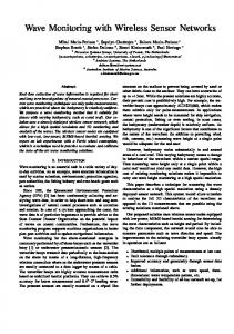
Fig. 1.
{(C,D)}
Operation of L INKS.
must be exchanged periodically. Depending on the network size and radio characteristics, this may require fragmentation into multiple packets, increasing overhead. Moreover, vector clocks are exchanged even in absence of configuration changes, wasting communication. This last observation motivates the design choices of the next protocol. IV. U SING LINK STATE INFORMATION At the other extreme, group membership information can be managed as “hard-state”, i.e., a node considers the group composition as stable until it receives a message saying otherwise. In this protocol, called L INKS, periodic messages to refresh state are not required, and nodes communicate only upon group configuration changes. To detect these, nodes rely on a lower-level neighbor discovery service, notifying the presence of new neighbors or the departure of existing ones. L INKS is independent of the neighbor discovery layer: any of the protocols in [5]–[9] can be used. Nevertheless, these generate their own traffic, which must be accounted for in the energy expenditure. We come back to this issue in Section VI, where we take into account the overhead introduced by Contiki’s neighbor discovery [19] used in our implementation. We take inspiration from link state routing protocols such as OSPF [20] and build each node’s view of the group by using topology information received from other nodes. Each node maintains a topology set summarizing all links in the network. Nodes run a topological sort on this set to determine all reachable nodes, i.e., the group members. Figure 1 illustrates how changes in the topology are discovered and propagated. In the example we assume nodes are initially connected in a chain and know all network links (step 1). For now, we also assume reliable links: later in this section we describe how communication faults are dealt with. Node leaving and joining. Whenever the underlying neighbor discovery layer notifies a neighbor departure, L INKS disseminates link information. For instance, upon the breakage of the link between B and C in step 2, both nodes broadcast a link update h#sequence, DROP, source, neighbori. Upon receiving an update tuple, a node checks its topology set to identify links that must be removed, and waits for a short time interval during which it buffers additional
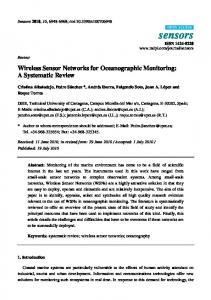
updates generated by the reconfiguration. Then, it packs the performed topology changes in as few messages as possible and broadcasts them. Any other receiving node repeats the process. Updates travel far away from the node that observed the change: in step 3, this process allows A to determine that C and D are no longer reachable, i.e., outside A’s group. Joining nodes are dealt with in a similar way. When a new neighbor is discovered, or a previously-broken link is reestablished as in step 4, the link end-points exchange updates in the form h#sequence, ADD, source, neighbori. In the figure, B notifies C about the existence of the link (A, B), allowing C to reconstruct the full topology. After the buffering interval, nodes re-propagate all changes in their topology set, e.g., in step 5 C broadcasts an update containing (A, B) and (B, C). A node receiving an update may determine that no changes to its topology set are required. This happens, for instance, in the case where updates about the same links, triggered by different nodes, are received by the same node through distinct paths. In this case, the node does not re-propagate the update, therefore avoiding unnecessary communication. Message failures. Unlike C LOCKS, in L INKS broadcasts are not idempotent and therefore cannot be sent repeatedly. Updates are generated and broadcast only once, i.e., when a change appears in a node’s topology set. Unfortunately, missing an update may lead to permanent errors. For instance, imagine that the update h#sequence, ADD, A, Bi in step 4 of Figure 1 is lost. As B will never re-broadcast the update, neither C nor D will become aware of A’s existence. To alleviate this problem, we implemented a positive acknowledgment scheme based on the update sequence numbers, ensuring reliable 1-hop broadcast. A node receiving an update (e.g., A in step 5) replies with a message containing a pair h#sequence, ACKi for all updates received in a predefined time window. If the update originator (B in this case) does not receive an acknowledgment from all of its neighbors in a given time frame, it repeats the operation for a limited number of times, hoping that the update is eventually received. � L INKS enjoys the desirable property that communication is proportional to the number of group changes. However, the need for reliability comes at a high cost, as described in Section VI. This problem is overcome by the next protocol. V. U SING DISTANCE VECTORS Our last protocol, called D IST, is inspired by distance vector routing protocols such as RIP [21]. Each node maintains a distance vector, i.e., a set of tuples hnode ID, next hop, minimum hop counti for every other node in the WSN. This information is managed as hard state, similarly to L INKS, therefore communication is required only upon group changes. Moreover, these are detected by an underlying neighbor discovery layer, as we already described in Section IV for L INKS. We rely on the example in Figure 2 to illustrate the operation of D IST, initially assuming reliable links. In step 1 the network is partitioned: A is out of range w.r.t. the group formed by B, C, and D. Nodes in the latter group have already exchanged their distance vector, represented as an array for simplicity. For
next hop for [A, B, C, D]
step
A
1
B [A, -, -, -] [0,∞,∞,∞]
hop count
A
B [A,B,B,B] [0,1,2,3]
A
3
C
B
B
[ -,C,C,D] [∞,2,1,0]
D [B,B,C,D] [2,1,0,1]
C [ -,B,C,C] [∞,0,1,2]
Fig. 2.
D
C
B [A, -, -, -] [0,∞,∞,∞]
[ -,C,C,D] [∞,2,1,0]
[B,B,C,D] [2,1,0,1]
[ -,B,C,C] [∞,0,1,2]
A
D
C [A,B,C,C] [1,0,1,2]
[A, -, -, -] [0,∞,∞,∞]
[ -,C,C,D] [∞,2,1,0]
[ -,B,C,D] [∞,1,0,1]
[C,C,C,D] [3,2,1,0]
D [ -,B,C,D] [∞,1,0,1]
B [A,B,B,D] [0,1,2,1]
D [ -,B,C,D] [∞,1,0,1]
[A,B,C,C] [1,0,1,2]
[A,B,B,B] [0,1,2,3]
A
5
C [ -,B,C,C] [∞,0,1,2]
2
4
A
distance vector broadcast
[C,C,C,D] [3,2,1,0]
Operation of D IST.
example, the one on B indicates that this node is 0 hops from itself, 1 hop from C, and 2 hops from D (reachable through C). The ∞ denotes that A is not a member of B’s group. Node joining. In step 2, node A approaches the group and the neighbor discovery layer notifies both A and B accordingly. The two nodes update and exchange their distance vectors in broadcast. B’s broadcast reaches also C, which identifies A as a new group member, reachable through B over 2 hops. Next, C updates its own distance vector with the proper hop count and broadcasts it (step 3), enabling D to discover A. Node leaving. When neighbor discovery notifies a node that a neighbor is no longer reachable, the node searches for alternative paths towards the departed node and the routes originally including it. If these exist, they include one of the remaining neighbors. If no alternative is found, the entry is purged from the distance vector. To find out, the node can either pull the distance vector from its neighbors or cache them locally. In our implementation, we chose the latter to limit complexity and communication overhead. For instance, upon A’s departure in step 4, neighbor discovery notifies A that B is no longer in direct radio range. As B was A’s only link to C and D, no alternative paths to these nodes exists and therefore their entries are purged from A’s distance vector. Similarly, B searches for alternative paths to A; its only option is a path through C. Still, this is invalid as B previously linked A and C. B is able to determine that the path is unsuitable by inspecting the next-hop field in the distance vector. Thus, B correctly purges A from its distance vector and broadcasts an update to its neighbors. The update allows C, after searching through the distance vector of its neighbors, to identify that no viable path to A exists. C prunes A from its distance vector and broadcasts an update (step 5). Eventually, D also evicts A, and the network reverts to the state in step 1. Handling loops. To avoid counting to infinity when loops occur, D IST measures the hop count to a destination on the shortest path. For instance, in step 3 B discards C’s broadcast due to its direct link to A, and correctly identifies A at 1 hop. Beyond a maximum hop count, a node is deemed unreachable. More interesting is the case of finding alternative paths over routing loops. Imagine a ring configuration as in Figure 3. At some point in time, the link (A, B) fails. According to
Fig. 3.
C [A,B,C,C] [1,0,1,2]
D [B,B,C,D] [2,1,0,1]
[A,C,C,D] [1,2,1,0]
D IST: finding alternative paths over loops.
the previous reasoning, B advertises an infinite distance to A, forcing C to discover the alternative path to A that passes through D. C advertises the found path further, and thus B identifies A as being still a member of the group. Message failures. For D IST to work properly, messages containing distance vectors cannot be lost. An easy solution is to retransmit them periodically, but all advantages over C LOCKS would be lost. However, unlike L INKS where updates are incremental, in D IST a single retransmission can make up for an earlier loss, restoring a node’s entire group view. Based on this observation, we employ a negative acknowledgment scheme that guarantees that nodes eventually update their distance vector in the correct way. A version number is associated to the distance vector of each node, incremented on every change and piggybacked on all broadcasts. Each node broadcasts periodically a digest, that is, a list of pairs hnode ID, last known version numberi. When another node receives a pair containing its identifier, it compares the received version number to its own—the true one. The receiving node is then able to determine gaps in the sequence, denoting that the sender missed earlier updates. If and only if this is the case, a rebroadcast of the full distance vector is required to bring the outdated node on par. VI. E VALUATION In this section we evaluate and compare our three protocols, implemented in Contiki [4], and simulated using COOJA [22]. We perform the evaluation in two settings. The first one is a synthetic scenario that allows us to control precisely the mobility patterns inside groups. The results gathered in this scenario, described in Section VI-A, are then validated in Section VI-B against simulations where the mobility patterns are instead derived from real-world GPS traces of humans. Goals. Our first objective is to assess the impact each protocol bears on the energy budget. In principle, one could use LPL [23] or other duty-cycling mechanisms in conjunction with our protocols, however biasing the overall energy figures. We decided to avoid this bias by performing our experiments with the radio always on and without taking into account the contribution of idle listening. Therefore, we compare protocols in their “purest” form, by focusing solely on the cost of message exchanges, and consequently by measuring energy consumption indirectly through the total number of bytes transmitted and received by each node: bitsRX bitsTX + IRX × ) b b For the popular TMote Sky platform we used in our experiments, V = 3 V, ITX = 21 mA, IRX = 23 mA, and b = 250 kbps [3]. For L INKS and D IST, our evaluation includes the traffic generated by the underlying neighbor discovery layer, in our case the one in Contiki’s RIME stack [19]. ∆
energy = V × (ITX ×
TABLE I P ROTOCOL PARAMETERS .
Description Beaconing period (for neighbor discovery and vector clock exchange) Timeout for declaring a neighbor missing Radio range C LOCKS Vector clock element size L INKS Update tuple size Minimum timespan between retransmissions Maximum retransmissions D IST Distance vector element size Digest retransmission period
A. Synthetic mobility patterns Value B ∈ {5, 10} s T = 120 s 30 m 2B 3B 1.5 s 5 3B D ∈ {30, 120} s
Our second objective is to evaluate the protocols’ accuracy, represented by two metrics: i) the error, i.e., the difference between the reported group size and the actual one— an instantaneous property whose value changes while protocols are detecting group changes; ii) the detection latency, i.e., the (average) delay between the group change and the time at which nodes become aware of it. The two metrics are related: given an initial error of zero, detection latency can be regarded as the time a protocol takes to bring the error back to zero after a group change occurs. Parameters. Key to the configuration of all protocols is the neighbor discovery latency, i.e., the delay after which a node becomes aware of the arrival or departure of a neighbor, which in turn may trigger a group membership change. There are two concerns that must be taken into account, as follows. First, while discovering a new neighbor is as simple as receiving a beacon from it, ascertaining a neighbor’s departure is significantly more difficult. Indeed, missing a beacon from a neighbor can be caused by movement, node crashes, or packet losses. In practice, neighbor discovery services declare a neighbor missing only after no beacons are received for a given predefined time interval T . In the discovery service we used [19], T =120 s. Second, the value of T affects the behavior of L INKS and D IST, which rely directly on neighbor discovery. However, in practice the configuration of C LOCKS is also affected by T , to ensure that results are comparable. We configured C LOCKS to identify departed nodes after the same timeout T = 120 s. Although the latter is managed as logical time, as described in Section III, this choice strikes the best tradeoff between a fair comparison and practical implementation concerns. We evaluate the impact of this value in more detail in Section VI-A2. We also match the vector clock broadcast rate with the beacon rate of the neighbor discovery service, noted hereafter B. We evaluate scenarios with B ∈ {5, 10} s. The D IST protocol has an additional parameter, namely the period D with which the digests are broadcast in our negative acknowledgment reliability scheme. We evaluate two instances of D IST, corresponding to D ∈ {30, 120} s. We show the other simulation and protocol parameters in Table I. The results for a given simulated scenario are averaged over 40 repetitions.
1) Energy consumption: We simulate our protocols using a 25-node group moving in a single direction with a constant velocity (1 m/s) for 3500 s, long enough to retrieve interesting insights about the protocols’ operation. Figure 4 illustrates our synthetic setting. The group is initially arranged in a grid configuration. Along the way, the group passes through a series of checkpoints (only one is illustrated). In between two consecutive checkpoints most nodes keep the same position within the group, except for a given, simulation-controlled number of nodes that swap positions, e.g., A and B. The swaps take place in between checkpoints, with the selected nodes moving at 1 m/s towards their target positions, and must complete at the destination checkpoint. At a checkpoint, a different set of nodes (e.g., C and D) are selected and begin swapping positions. Note that, in this scenario the group members change their positions within the group, but the group does not change its composition, i.e., no node joins or leaves the group. Indeed, our objective in this section is to analyze the impact of mobility alone on group maintenance. We analyze joining and leaving nodes in Section VI-A2, as this bears a direct impact on the accuracy of our protocols. Our synthetic scenario allows us to define a simple measure of the churn caused by mobility, as a combination of number of swaps and the distance between consecutive checkpoints: ∆
churn =
number of position swaps × 100 distance between checkpoints
We setup simulations for all dimensions affecting churn. The first one is the distance between checkpoints, which we consider to be either 10, 50, or 100 m. The second dimension is the number of position swaps: we take into consideration groups without swaps and groups experiencing 1 to 5 swaps between checkpoints. The last dimension we explore is the network density, which we control through the relationship between the grid unit (distance between nodes) and the radio range that, as shown in Table I, is fixed to 30 m. The configurations we simulate are: • a “sparse” one where the grid unit of 15 m allows nodes to communicate 2 hops (grid units) away. • a “dense” one where the grid unit of 8 m allows nodes to communicate 3 hops (grid units) away. The combination of all these parameters yields 64 different simulated scenarios per protocol, each repeated 40 times. Results. Figure 5 compares the protocols for churn = 20, corresponding to 2 position swaps every 10 m. In all scenarios, L INKS is the most energy-hungry among our protocols, especially in the case of a dense network. Logs show that the culprit for the high consumption is the acknowledgment scheme ensuring reliable broadcast. In fact, approximately 40% of the traffic is due to acknowledgments and retransmissions. Figure 5 also shows that the impact of the B parameter is bigger in C LOCKS than in D IST. This, however, is expected. In C LOCKS, B represents the period with which vector clocks are exchanged, and thus bears a direct influence on traffic, and
A
D B
C
START
CHECKPOINT
STOP
1 m/s
1 m/s
0.8 0.6 0.4 0.2 0
Our synthetic scenario for group movement. Energy (mJ)
Energy (mJ)
Fig. 4. LINKS CLOCKS
DIST(30)/ DIST(120) 0
500
1000
1500 2000 Time (s)
2500
3000
0.8 0.6 0.4 0.2 0
3500
LINKS
CLOCKSDIST(120) 0
LINKS CLOCKS
0
500
1000
1500 2000 Time (s)
DIST(30)/ DIST(120)
2500
500
1000
1500 2000 Time (s)
2500
3000
3500
(b) dense network, B = 10 s. Energy (mJ)
Energy (mJ)
(a) dense network, B = 5 s. 0.8 0.6 0.4 0.2 0
DIST(30)
3000
0.8 0.6 0.4 0.2 0
3500
LINKS DIST(30)
0
500
1000
DIST(120) CLOCKS
1500 2000 Time (s)
2500
3000
3500
(c) sparse network, B = 5 s. (d) sparse network, B = 10 s. Fig. 5. Cumulative energy for churn = 20, corresponding to 2 swaps every 10 m. 1.4
1.4 1.2
DIST(30) DIST(120) LINKS CLOCKS
1 0.8
Power (uW)
Power (uW)
1.2
0.6 0.4 0.2
DIST(30) DIST(120) LINKS CLOCKS
1 0.8 0.6 0.4 0.2
0
0 0
10
20
30
40
50
0
10
-1
(a) dense network, B = 5 s.
30
40
50
(b) dense network, B = 10 s.
1.4
1.4
1.2
1.2
DIST(30) DIST(120) LINKS CLOCKS
1 0.8
Power (uW)
Power (uW)
20
Churn (m-1)
Churn (m )
0.6 0.4 0.2
DIST(30) DIST(120) LINKS CLOCKS
1 0.8 0.6 0.4 0.2
0
0 0
10
20
30
40
50
-1
(c) sparse network, B = 5 s. Fig. 6.
0
10
20
30
40
50
Churn (m-1)
Churn (m )
(d) sparse network, B = 10 s. Power consumed as a function of churn.
in turn energy consumption. Instead, in D IST B is the beacon period used for neighbor discovery, which is only a fraction of the total traffic: the update and recovery messages in the network cannot be directly correlated to changes in the local neighborhood, yielding a reduced influence of B. Figure 5 also highlights the impact of density on energy consumption. For the dense scenario, each broadcast (i.e., a neighbor discovery beacon or the transmission of a vector clock, link update, or distance vector) reaches more nodes and therefore consumes more battery w.r.t. sparser networks. We now turn our attention to the impact of churn (i.e., mobility) on energy consumption. Instead of plotting the cumulative energy for all the aforementioned 64 scenarios covering all parameter combinations, we chose to analyze the slope ∆energy/∆time of the energy curves (i.e., the power consumed) as a function of churn, as shown in Figure 6. This approach is more concise, and captures effectively the impact of mobility on energy consumption. These charts report
results only for the time interval between 500 and 3500 s, to exclude the initial traffic required to “bootstrap” a network with an empty group view. Also, note that the “humps” around churn = 10 (evident for L INKS but present also in the other protocols) is caused by the non-linearity of our definition of churn. For instance, churn = 8 may correspond to 4 swaps every 50 m, and churn = 10 to a single swap every 10 m. The charts in Figure 6 show that L INKS is greatly affected by churn even in a static dense group, and becomes a viable alternative only for quasi-static groups in the sparse configuration. In our dense configuration, the energy consumption of L INKS is dominated by the reliability scheme, due the increased likelihood of collisions. On the other hand, the performance of C LOCKS and D IST is very similar for B = 5 s, where the short periodicity (of beacons and vector clock exchanges) affects directly the overhead. For B = 10 s, instead, D IST has an extra overhead caused by the exchange of distance vectors and their recovery, the latter clearly more
discovery
60
propagation
discovery
60
propagation
50
50
40
40
40
30 LINKS 20 10
DIST(30)
30 LINKS 20
DIST(30)
DIST(120) 10
CLOCKS
CLOCKS
350
discovery
400 Time (s)
450
0 500 300
350
LINKS 20
DIST(120) 10
DIST(30) CLOCKS
Fig. 7.
400
450
(b) 40% nodes leave. Error and detection latency vs time (B = 10 s).
marked in the dense scenario. 2) Error and detection latency: As mentioned at the beginning of Section VI, detecting node departure is more difficult than detecting node join. Consequently, we design our scenario around node departures and use it to measure accuracy. We start from a 25-node network displaced randomly in a 100×100 m2 area, with a radio range of 30 m. The network bootstraps and identifies all group members. Then, at 300 s, a number of randomly-selected nodes are suddenly separated from the rest of the network, creating a new partition. This actually represents a worst-case w.r.t. the more realistic scenario where nodes move away, instead of being instantaneously relocated, because in the former case the departure can be discovered gradually. We perform simulations where 25%, 40%, and 60% of the nodes are separated from the main group. Results. Figure 7 illustrates the accuracy of our protocols by showing i) how the error changes over time, and ii) the detection latency, i.e., the time necessary to reconstruct a correct group view on all nodes. We show only the experiments with B = 10 s, as those with B = 5 s yield similar results. L INKS and D IST both rely on the neighbor discovery layer for detecting the departed nodes. Nevertheless, as discussed earlier, this layer declares a neighbor as unavailable only upon a timeout, whose value in the RIME stack is T = 120 s. This explains the constant error in the initial part of curves: only at 420 s the nodes, alerted by the neighbor discovery layer, begin the propagation of information of the group change. The same timeout is used for C LOCKS, but in this case there are two interesting differences: i) in L INKS and D IST, no action other than local neighbor discovery is taken until the timeout T expires. Instead, in C LOCKS the nodes continuously propagate their vector clocks with a period B < T , therefore actively and continuously cooperating in reconstructing the global view; ii) recall that in C LOCKS the (logical) clocks in the network continuously realign themselves to the largest one. Therefore, it is as if “time runs faster” for C LOCKS, reaching the deadline set by T faster than in physical time. The net effect of the considerations above is that, in all configurations of Figure 7, C LOCKS is much faster than the other protocols in converging to a consistent group view. However, this should not be taken as a direct comparison given that, in the absence of better choices, we use the same T = 120 s for both physical and logical time, and therefore a direct comparison is somewhat biased. In principle, one could
DIST(120)
latency
0 500 300
Time (s)
(a) 25% nodes leave.
propagation
30
latency
latency
0 300
Error (%)
50
Error (%)
Error (%)
60
350
400
450
500
Time (s)
(c) 60% nodes leave.
set the value of T appropriately for L INKS and D IST, to reduce their initial “waiting time”; indeed we have simulations for T = 30 s which show a much shorter initial plateau for these protocols. Still, because of the first consideration above, during this time C LOCKS actively works to reconcile the global view: this is an intrinsic property of the protocol that may help speed up convergence w.r.t. L INKS and D IST when these use relatively high values of T . Remember that if T is too small, packet losses are mistaken for neighbor departures. Figure 7 shows another interesting difference between C LOCKS and the other two protocols, in terms of how the network converges to the same global view, ultimately determining the group detection latency. Detection latency is a function of the number of hops in the network, but the delay at each hop depends on the protocol. In C LOCKS, the global view of all nodes is maintained in synchronous steps: as evidenced in the figure, convergence occurs by an alternation of plateaus (where nodes wait for T to expire) and bursts of node evictions. Instead, the other two protocols propagate the global information entirely asynchronously, at a faster pace but with longer tails. B. Real-world GPS traces We now seek validation of the results in our synthetic scenarios through experiments on real-world GPS traces. We use the CRAWDAD KAIST data [24] representing daily records of students in a university campus over 3 months. We pick randomly 25 out of the 92 traces, and scale them into a 300×300 m2 area. We use B = 10 s and a 30 m radio range. Due to the nature of the traces, the scenario is very challenging because i) nodes are continuously moving, i.e., the system never stabilizes; ii) nodes move of their own volition, not as a group: therefore, the ratio of joining and leaving nodes is much higher than in the applications we target. The energy consumption is reported in Figure 8(a) along with the average number of neighborhood changes. We notice trends similar to Figure 5: an excessive overhead for L INKS, similar performance of C LOCKS and D IST, a slightly better performance of D IST (120) due to the lighter recovery traffic. More interesting is the error, reported in Figure 8(b) along with neighborhood changes. Because nodes are continuously moving at a high rate the error never stabilizes at zero, unlike the experiments in Section VI-A2. This is also the reason why the detection latency is not shown, as it cannot be computed. Nevertheless, the chart is interesting because the three protocols exhibit very different behaviors. L INKS is
Energy (mJ)
1.5 LINKS
1 0.5 0 0
500
Neighborhood changes
22 20 18 16 14 12 DIST(30) 10 DIST(120) 8 CLOCKS 6 4 2 0 1000 1500 2000 Time (s)
neighborhood changes 2
40 35 30 25 20 15 10 5 0 0
Fig. 8.
22 20 18 16 14 12 LINKS DIST(30) DIST(120) CLOCKS 10 8 6 4 2 0 500 1000 1500 2000 Time (s)
neighborhood changes
Neighborhood changes
Error (%)
(a) Cumulative energy.
(b) Error Experiments with the real-world GPS traces in [24].
able to reduce progressively the error and stabilize it around 10-15%. In contrast, both versions of D IST cannot keep up with the mobility rate, although they have the same B and T configuration of L INKS: their error appears to grow with time. The best performance is achieved by C LOCKS, which keeps the error very close to zero despite the high mobility. VII. C ONCLUSION AND F UTURE W ORK In this paper we tackled the problem of monitoring groups of mobile nodes equipped with WSN devices, a problem that has hitherto received little attention. We presented and compared three protocols covering a big fraction of the solution space. Our study indicates that C LOCKS is resilient to the changes induced by mobility, has comparatively low energy demands and quick convergence time. C LOCKS is the protocol of choice if the sole goal of the network is to monitor groups. However, in many mobile WSN applications a neighbor discovery service is necessary for other purposes. For instance, in our applications it is used to detect proximity to hazards or log “contacts” with other mobile nodes. If this is the case, the D IST protocol allows one to build upon this already-present functionality with promising results: D IST has energy demands comparable to C LOCKS (and even lower for slowly-changing groups) and, if properly configured, can achieve similarly fast convergence, although this aspect must be studied further. This issue is already on our research agenda, along with a concrete test of C LOCKS and D IST in the real-world deployments we concisely discussed in Section I, namely, the care of Alzheimer’s patients, and the study of the social behavior of roe deer. ACKNOWLEDGMENTS The work described in this paper was partially supported by the Autonomous Province of Trento under the call for proposals “Major Projects 2006” (project ACUBE) and by the EU Cooperating Objects Network of Excellence (CONET: FP7-2007-2-224053).
R EFERENCES [1] F. Cagnacci, L. Boitani, R. A. Powell, and M. S. Boyce, “Animal ecology meets GPS-based radiotelemetry: a perfect storm of opportunities and challenges,” Philosophical Transactions of The Royal Society Biological Sciences, vol. 365, no. 1550, 2010. [2] D. Lusseau and M. E. J. Newman, “Identifying the role that individual animals play in their social network,” Proc. R. Soc. London B (Suppl.), vol. 271, 2004. [3] Sentilla, “TMote Sky Datasheet,” http://www.sentilla.com/moteivtransition.html, accessed on 1/2011. [4] A. Dunkels, B. Gronvall, and T. Voigt, “Contiki - a lightweight and flexible operating system for tiny networked sensors,” in Proc. of the 1st IEEE Workshop on Embedded Networked Sensors (Emnets-I), 2004. [5] P. Dutta and D. Culler, “Practical asynchronous neighbor discovery and rendezvous for mobile sensing applications,” in Proc. of the 6th Int. Conf. on Embedded network sensor systems (SenSys), 2008. [6] A. Kandhalu, K. Lakshmanan, and R. Ragunathan, “U-Connect: A lowlatency energy-efficient asynchronous neighbor discovery protocol,” in Proc. of the 9th Int. Conf. on Information Processing in Sensor Networks (IPSN), 2010. [7] M. J. McGlynn and S. A. Borbash, “Birthday protocols for low energy deployment and flexible neighbor discovery in ad hoc wireless networks,” in Proc. of the 2nd Int. Symp. on Mobile ad hoc networking & computing (MobiHoc), 2001. [8] Y.-C. Tseng, C.-S. Hsu, and T.-Y. Hsieh, “Power-saving protocols for IEEE 802.11-based multi-hop ad hoc networks,” Comput. Netw., vol. 43, no. 3, 2003. [9] R. Zheng, J. C. Hou, and L. Sha, “Asynchronous wakeup for ad hoc networks,” in Proc. of the 4th Int. Symp. on Mobile ad hoc networking & computing (MobiHoc), 2003. [10] N. Sridhar, “Decentralized local failure detection in dynamic distributed systems,” in Proc. of the 25th IEEE Symp. on Reliable Distributed Systems (SRDS), 2006. [11] A. Jhumka and L. Mottola, “On consistent neighborhood views in wireless sensor networks,” in Proc. of the 28th IEEE Symp. on Reliable Distributed Systems (SRDS), 2009. [12] K. P. Birman and T. A. Joseph, “Reliable communication in the presence of failures,” ACM Trans. Comput. Syst., vol. 5, no. 1, 1987. [13] R. Vitenberg, I. Keidar, G. V. Chockler, and D. Dolev, “Group communication specifications: A comprehensive study,” ACM Computing Surveys, vol. 33, no. 4, 1999. [14] G.-C. Roman, Q. Huang, and A. Hazemi, “Consistent group membership in ad hoc networks,” in Proc. of the 23rd Inter. Conf. on Software Engineering (ICSE), 2001. [15] P. Juang, H. Oki, Y. Wang, M. Martonosi, L. S. Peh, and D. Rubenstein, “Energy-efficient computing for wildlife tracking: design tradeoffs and early experiences with ZebraNet,” SIGARCH Comput. Archit. News, vol. 30, no. 5, 2002. [16] V. Dyo, S. A. Ellwood, D. W. Macdonald, A. Markham, C. Mascolo, B. P´asztor, S. Scellato, N. Trigoni, R. Wohlers, and K. Yousef, “Evolution and sustainability of a wildlife monitoring sensor network,” in Proc. of the 8th Conf. on Embedded Networked Sensor Systems (SenSys), 2010. [17] F. Mattern, “Virtual time and global states of distributed systems,” in Proc. Workshop on Parallel and Distributed Algorithms, 1989. [18] M. Mar´oti, B. Kusy, G. Simon, and A. L´edeczi, “The flooding time synchronization protocol,” in Proc. of the 2nd Int. Conf. on Embedded networked sensor systems (SenSys), 2004. ¨ [19] A. Dunkels, F. Osterlind, and Z. He, “An adaptive communication architecture for wireless sensor networks,” in Proc. of the 5th Int. Conf. on Embedded Networked Sensor Systems (SenSys), 2007. [20] J. Moy, “OSPF Version 2,” IETF, 1998. [21] C. Hedrick, “Routing Information Protocol,” IETF, 1988. ¨ [22] F. Osterlind, A. Dunkels, J. Eriksson, N. Finne, and T. Voigt, “Crosslevel sensor network simulation with COOJA,” in Proc. of the 1st Int. Workshop on Practical Issues in Building Sensor Network Applications (SenseApp 2006), 2006. [23] J. Polastre, J. Hill, and D. Culler, “Versatile low power media access for wireless sensor networks,” in Proc. of the 2nd Int. Conf. on Embedded networked sensor systems (SenSys), 2004. [24] I. Rhee, M. Shin, S. Hong, K. Lee, S. Kim, and S. Chong, “CRAWDAD trace ncsu/mobilitymodels/gps/kaist (v. 2009-07-23),” From http://crawdad.cs.dartmouth.edu/ncsu/mobilitymodels/GPS/KAIST.