group-sma algorithm based joint estimation of train parameter and state

W. Zheng, J. Han, W. Kong, L. Wang: Group-SMA Algorithm Based Joint Estimation of Train Parameter and State

WEI ZHENG, Ph.D. Corresponding author E-mail: [email protected] JUAN HAN E-mail: [email protected] WEIJIE KONG E-mail: [email protected] LIXIANG WANG E-mail: [email protected] National Engineering Research Center of Rail Transportation Operation and Control System, Beijing Jiaotong University No.3 Shangyuancun, Xizhimenwai, Haidian District, Beijing, 100044, China

Transport Technology Review Submitted: Mar. 20, 2014 Approved: Feb. 3, 2015

GROUP-SMA ALGORITHM BASED JOINT ESTIMATION OF TRAIN PARAMETER AND STATE

ABSTRACT The braking rate and train arresting operation is important in the train braking performance. It is difficult to obtain the states of the train on time because of the measurement noise and a long calculation time. A type of Group Stochastic M-algorithm (GSMA) based on Rao-Blackwellization Particle Filter (RBPF) algorithm and Stochastic M-algorithm (SMA) is proposed in this paper. Compared with RBPF, GSMA based estimation precisions for the train braking rate and the control accelerations were improved by 78% and 62%, respectively. The calculation time of the GSMA was decreased by 70% compared with SMA.

KEY WORDS parameter estimation; state estimation; particle filter; rail braking system;

1. INTRODUCTION With the high-speed development of rail transportation, the safety and efficiency requirements during the transport process are increasing. Urban train parking precision affects the alignment of the train door with the platform screen door (PSD). The train braking system is a crucial factor affecting the parking accuracy. The braking rate is affecting the performance of the train braking system. The long-time continuous operation and the variation of the loading conditions and operation system will lead to the inevitable change of the braking rate. The displacement and velocity measurement accuracy is affecting the braking accuracy and it Promet – Traffic&Transportation, Vol. 27, 2015, No. 1, 85-95

is affected by the performance of the velocity sensors. The aforementioned precision problems can be converted to the joint estimation of unknown parameter and states by modelling the train braking process. In the train braking model, the velocity and displacement are states in the state space model, and the braking rate is the unknown parameter to be estimated. The commonly used parameter identification methods are point estimation algorithms and filtering algorithms [1]. The traditional point estimation algorithms contain the least squares [2], maximum likelihood estimation method [3] and EM algorithm (Expectation Maximization) [4]. When the point estimation algorithms are used for the parameter estimation, it requires that the objective function is continuous and derivable. The estimated parameter value is searched by the gradient information, so it easily falls into the local minimum. The parameter identification method based on neural network [5] has the ability to approximate non-linear functions with arbitrary precision, but there are still several problems such as the determination of the network structure, sample data selection and network training algorithms. Genetic algorithm [6] has defects of premature or slow convergence. The Kalman filter and extended Kalman filter (EKF) have been applied successfully in the state estimation [7]. The Interacting Multiple Model (IMM) algorithm [8] is based on Kalman Filter (KF) and it has been used for the state estimation of the hybrid system. Knowledge of the transition probability between different models must be achieved in advance, which is difficult in practical engineering. 85

W. Zheng, J. Han, W. Kong, L. Wang: Group-SMA Algorithm Based Joint Estimation of Train Parameter and State

The Particle Filter (PF) uses the non-parametric Monte Carlo method to achieve the recursive Bayesian filter. This algorithm is suitable for any non-linear systems that can be modelled by state space equation and its estimation precision is approximate to the optimal estimation. N. Metropolis and S. Ulam in [9] proposed a particle filter for the first time. Development of the particle filter is introduced in [10] and its application in sensor diagnosis and accident detection in [11, 12]. There exist two major defects of the method. Firstly, the particle diversity decreases after several steps and all the particles tend to be of the same value. The Auxiliary particle filter (APF) and Gaussian particle filter (GPF) were discussed to solve this problem in [13]. The second problem is that the particle filter needs a large number of samples to approximate the posterior density of the system state. Rao-Blackwellization technology in [14] reduces the number of particles by reducing the dimension of the state vector. In RBPF algorithm, the state space is divided into linear substate space estimated by Kalman filter algorithm and non-linear sub-state space estimated by particle filter algorithm [15-18]. The RBPF has applications in the hybrid Gaussian [19-21], fixed parameters estimation [22], hidden Markov models (HMMs) [20-21], Dirichlet process models and Dynamic Bayesian Networks (DBN) [23]. There is no transition function for the unknown parameter in the state space equations. After several steps of the iterative calculation, all values of the parameter particles will tend to the same if the RBPF algorithm is used for the joint train braking rate estimation and the train states. SMA [24] is more efficient than RBPF for the state estimation of the hybrid system. SMA originally grows from the stochastic Malgorithm [25], based on a random sampling. In the SMA algorithm, the unknown parameter is discrete in several values and each discrete value corresponds to a system mode. When each parameter particle is predicted, the particle is transferred to all the possible discrete values from the unknown parameter, leading to an exponential growth of the particles number. The GSMA is proposed to reduce the computation complexity, keeping the estimation precision. The second part of this paper introduces the principle of the estimation algorithms for the hybrid system. The GSMA is proposed in the third part. After the train braking model is specified in the fourth part, the RBPF algorithm, the SMA algorithm and the GSMA are employed for the joint estimation of train braking rate and states in the fifth part. Advantages and limitations of the GSMA algorithm are given in section six.

2. PROBLEM FORMULATION Train braking system main function is to achieve consistent braking performance by a brake control86

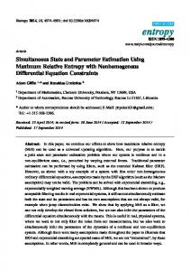
ler. The driver completes the vehicle control using the vehicle traction control system and the brake control system, but the driver cannot directly manipulate the train power actuators. The brake model is a vehicle operating model including train braking control system [26-28]. The target acceleration has the fixed linear relationship with the drive input so it is chosen as the input of the braking controller and represented by aTar ^ t h . The brake controller will track aTar ^ t h by feedback regulation. The dynamic regulation process is described as Equation (1): 1 f (1) ato ^ t h = - x at ^ t h + x aTar ^t - T h where at ^ t h denotes the control acceleration and it is the output of the controller, ato ^ t h means the derivation of at ^ t h after value t and f represents the braking rate which is defined as the ratio of the actual braking power with the expected braking power. The nominal value of f is 1, meaning the actual braking power is ideally equal to the expected braking power. Response time of the power actuator x represents the time needed for the braking power to reach the desired value. Transmission delay time from the generation of the target acceleration to the execution of the power actuator is T, so aTar ^t - T h denotes the execution of the target acceleration with aTar ^t - T h = 0 where t # T . The accumulated acceleration of the vehicle is denoted by vo ^ t h and it can be calculated from at ^ t h and additional acceleration caused by the bends and gradients of the railroad track, denoted by d ^ t h : (2) vo ^ t h = at ^ t h + d ^ t h The displacement of the urban railway is represented by D ^ t h and it is calculated from the velocity represented by v ^ t h : (3) Do ^ t h = v ^ t h Equations, from (1) to (3), describe the relationships between the target acceleration rate and the train operation status consisting of the acceleration, velocity and displacement. The corresponding block diagram of urban train braking model is presented in Figure 1. Notation 5 represents the input signals point. The Laplace linear operator of function f ^ t h with a real argument t ^t $ 0h , transforms f ^ t h to function F^ sh =

3

#

0

f ^ t h e -st dt

with complex argument s. After Laplace transformation, differentiation and integration become multiplica-1 x aTar ^t - T h f x

ato ^ t h

d^ t h

#

at ^ t h

vo ^ t h

#

v^ t h

#

D^ t h

Figure 1 - Block diagram of urban train braking model

Promet – Traffic&Transportation, Vol. 27, 2015, No. 1, 85-95

W. Zheng, J. Han, W. Kong, L. Wang: Group-SMA Algorithm Based Joint Estimation of Train Parameter and State

tion and division in polynomial equations. The inverse Laplace transformation reverts the solution to the time domain. The Laplace transformation of Figure 1 is shown as Figure 2. d^ sh aTar ^ s h

e -Ts

at ^ s h f xs + 1

1 v^ sh 1 D^ sh s s

Here 1/s represents the integration element and f/ ^xs + 1h is the inertial transfer function in the Laplace space. Value e -Ts denotes delay of T in the Laplace space, approximated with ^- s + mh / ^ s + mh . Figure 1 is now approximated by Figure 3(a) and then by Figure 3(b) [26]. d^ sh at ^ s h f xs + 1

1 v^ sh 1 D^ sh s s

Figure 3(a) - Approximation transfer block of urban train braking model d^ sh aTar ^ s h

at ^ s h f xs + 1

-1 2m s+m

1 v^ sh 1 D^ sh s s

y = Cx

T x = 7D v at azA

T

E = 60 1 0 0@T JK1 0 0 0NO K O (4)1 C = KKK0 1 0 0OOO . KK OO 0 0 0 1 L P JK0 1 0 0 NO KK O KK0 0 1 0 OOO A = KK 1 fO KK0 0 - x x OOO KK O 0 0 0 - mO L P Here x represents the state vector of the system, y denotes the observation vector of the system and m is a parameter related to the transmission delay time T. The system coefficient matrices are A, b, E and C and X represents the process Gaussian noise. The train braking model was demonstrated and verified with the practical operation data of YIZHUANG subway line in Beijing in literature [28]. As can be seen in the state space model, there are parameters m , x , f to be estimated. Static parameters m and x are estimated through offline methods.

3. PRESENTATION OF GSMA ALGORITHM The hybrid system, particle filter algorithm, SMA and GSMA algorithms are presented further in the text.

az ^ s h

Figure 3(b) - Equivalent transfer block of urban train braking model from Figure 3(a)

3.1 Hybrid system

Here value m is an introduced coefficient calculated from T with the Pade ^ h function in Matlab Software and az ^ s h is considered as the value derived from aTar ^ s h [26]. Displacement D ^ t h velocity v ^ t h , control acceleration at ^ t h and intermediate variables az ^ t h are selected as the state variables. By inverse Laplace transformation, values from Figure 3(b) are transformed to Figure 4. Function d ^ t h is assumed as the process Gaussian noise and it is denoted by scalar X ^ t h . Assum-

2m

ao z ^ t h

The state of the hybrid system ^ik, xk h is composed of parameter ik and the state xk . Each system model corresponds to a set of state space equations containing state transition equations and observation equations: (5) ik + 1 + p ^ik + 1 ik h (6) xk + 1 = { ^ik h xk + B ^ik h uk + C ^ik h wk 1.

In this formula T represents the transposition for the rows with columns. -1 x

-m aTar ^t h

T

f b = ;0 0 - x 2mE

Figure 2 - Laplace transformation blocks of urban train braking model

aTar ^ s h - s + m s+m

ing that x = 7D v at azA and y = 7D v azA , the state space equations of the model can be described as: xo = Ax + bat + EX

#

az ^ t h

f x

ato ^ t h

d^ t h

#

at ^ t h

vo ^ t h

#

v^ t h

#

D^ t h

-1

Figure 4 - Inverse Laplace transformation from Figure 3(b)

Promet – Traffic&Transportation, Vol. 27, 2015, No. 1, 85-95

87

W. Zheng, J. Han, W. Kong, L. Wang: Group-SMA Algorithm Based Joint Estimation of Train Parameter and State

(7) yk = H ^ik h xk + vk Here, ik + 1 represent the value of the discrete system parameter at discrete moment k + 1 . The input value of the system at moment k is uk . The probability transition matrix of discrete parameters is p ^ik + 1 ik h . The system coefficient matrices are { ^ik h , B ^ik h , C ^ik h and H ^ik h . Process noise and measurement noise at moment k are ~k and vk and both are the independent white Gaussian noise. Parameter ik + 1 is calculated from the probability transition matrix p ^ik + 1 ik h by (5). The continuous state transition equation and observation equation are (6) and (7), respectively. The state estimation is in calculating the parameter and state posterior probability density p ^ik, xk Y1: k h , where Y1:k describes the system measurements from moment 1 to moment k in steps.

3.2 Particle Filter algorithm (1) Filter is sequential to estimate parameter i and state x of a system given a set of observation variables. Variable z is used to represent the parameters and states variables set "i, x , . The posterior probability density of z for i = 0, 1, f, k - 1, k is estimated by the given observation process values yi , which presents the value of y at moment i, i = 0 , 1 , f, k - 1 , k . (2) Particle filters use a large random number of sample points sampled from the sampling function in the state space to approximate the posterior probability distribution of the estimated variables. (3) The procedures of particle filters are as follows [20]: 1) For draw samples from i = 1, f, N , ^i h ^i h zk + p _ zk zk - 1 i . Here N is the number of the sample particles. 2) For i = 1, f, N , update the importance weights by ^i h ^i h ^i h ~t k = ~k - 1 p _ yk zk i , 3) For i = 1, f, N , normalize the importance weights by ^i h ~t ^i h ~k = N k / _~t ^ki hi2 i=1

4) Compute an estimation of the effective number of particles Nt eff by: 1 Nt eff = N / _~t ^ki hi2 i=1

5) If the effective number of particles Nt eff is less than the given threshold Nthr , then resample in steps: (a) Draw N particles from the current particle set with probabilities proportional to their weights. Replace the current particle set with the new one. ^i h (b) For i = 1, f, N , set ~k = 1/N 6) go back to step 2). 88

3.3 RBPF algorithm RBPF algorithm is commonly used for parameter and state estimation of hybrid system. From the Bayesian theory, the state posterior probability density function p ^ik, xk Y1: k h can be decomposed: p ^ik, xk Y1: k h = p ^ xk Y1: k, ik h p ^ik Y1: k h

(8)

The numerical solution of p ^ik Y1: k h can be approximately calculated through the particle filter algorithm. Given the available parameter values and the state coefficient matrices of the system, the analytic solution of p ^ xk Y1: k, ik h can be derived using Kalman filter algorithm. If the particle filter is used to estimate ^ jh the unknown parameter, p _ik i1: k - 1, Y1: k i is chosen as the sampling function to approximate the unknown posterior probability density function of the parameter. The parameter particles are obtained based ^ jh on p _ik i1: k - 1, Y1: k i and then the probability density function of p ^ik Y1: k h in (8) can be estimated. Func^ jh tion p _ik i1: k - 1, Y1: k i denotes the probability density function of the unknown parameter ik given the his^ jh tory values of the parameter particle i1:k - 1 and observations Y1:k . According to the theory of probability, ^ jh p _ik i1: k - 1, Y1: k i can be simplified as [12]: p _ik i1: k - 1, Y1: k i \ ^ jh ^ jh ^ jh    \ p _ yk ik , i1: k - 1, Y1: k - 1 i p _ik i1: k - 1, Y1: k - 1 i ^ jh

   = p _ik i1: k - 1 i # p _ yk, xk ik, i1: k - 1, Y1: k - 1 i dxk ^ jh

^ jh

   = p _ik i1: k - 1 i $

(9)

^ jh

     $ # p ^ yk xk, ik h p _ xk ik, i1: k - 1, Y1: k - 1 i dxk ^ jh

The border of the integral is the value space of xk . ^ jh Values ik denote the j-th particle estimation values at moment k. If the mean of the observation values and variance of measurement noise vk in (7) are denoted by H ^ik h xk and Qv , respectively, then p ^ yk xk, ik h is expressed as: p ^ yk xk, ik h = N ^H ^ik h xk, Qv h

(10)

In formula (9), p _ xk ik, i1: k - 1, Y1: k - 1 i is derived through the Kalman filter algorithm as [12]: p _ xk

^ jh

ik, i1: k - 1, Y1: k - 1 i = N ` xtk

^ jh

^ jh k - 1, P k k - 1 j

^ jh

^ jh

^ jh ^ jh ^ jh ^ jh xtk k - 1 = { _ik i xk - 1 + B _ik i uk ^ jh

Pk

k-1

^ jh ^ jh ^ jh ^ jh ^ jh = { _ik i Pk - 1 {T _ik i + C _ik i Q~ CT _ik i ^ jh

(11)

^ jh

where xk and ik represent the state particles and parameter particles of the system at moment k. Here, ^ jh ^ jh xtk k - 1 and Pk k - 1 represent the predicted state mean ^ jh and variance of state xk , respectively for the given ^ jh state xk - 1 . The variance of process noise wk in (6) is Q~ . From Equations (9) to (11), the sampling function can be parsed as: p `i k

^ jh

k - 1, Y1: k j

^ jh

i1

^ jh \ N ` ytk k - 1, C ^ykj hk - 1 j

(12)

Promet – Traffic&Transportation, Vol. 27, 2015, No. 1, 85-95

W. Zheng, J. Han, W. Kong, L. Wang: Group-SMA Algorithm Based Joint Estimation of Train Parameter and State

where

^ jh

ytk

k-1

= H _ik i xtk ^ jh

^ jh

k-1

,

C yk k - 1 = H _ik i Pk k - 1 H _ik i + Qw and the weights of the particles are calculated from: ^ jh

^ jh

^ jh

T

^ jh

^ jh ^ jh ^ jh ^ jh ^ jh ^ jh wk = p _ yk ik i p _ik ik - 1 i /p _ik ik - 1, Y1: k - 1 i

   \ / p _ yk ik , i1: k - 1, Y1: k - 1 i p _ik ^ jh

^ jh

sk

^ jh

^ jh

i1: k - 1 i ^ jh

(13)

   \ / p _ yk ik , i1: k - 1, Y1: k - 1 i ^ jh

sk

^ jh

^ jh

^ jh

Here wk represents the weight of the j-th particle at moment k and the system hybrid state estimation is obtained from the weighted sum of particle weights and particle values. The mean and variance of continuous state corresponding to each particle can be derived using the Kalman filtering algorithm. The posterior probability density function of xk can be expressed as a mixture of Gaussian function. The particle will show the degradation property if RBPF is used for the joint estimation of unknown parameter and system states because most of the parameter particles tend to transfer to the same discrete value after sampling step according to the sampling function, as the unknown parameter does not have the transition function. During the resampling process, the particles with large weights are replicated many times while the particles with small weights are rejected, and the replicated particles represent the samples. After several re-sampling steps, all the values of the parameter particles tend to be the same.

3.4 SMA algorithm The SMA algorithm is derived from the M-algorithm to solve the particle degradation problem occurring in the RBPF algorithm. The unknown parameter i in RBPF is assumed as discrete in M + 1 values "i^0h, i^1h, f, i^Mh,^M $ 0h . Discrete values represent the value space and any particle for i should belong to the value space. In each moment step from 0 to k, the parameter particle needs to be updated based on ^i h the sampling function. If the parameter particle ik - 1 is sampled at moment k - 1 , the transition probability ^i h from parameter particle ik - 1 to all possible discrete ^0h ^1 h ^Mh values in "i , i , f, i , is calculated first and then the parameter value corresponding to the largest transition probability is sampled as the parameter particle ^i h ik . In each particle trajectory, although there are M ^i h possible values to which parameter particle ik - 1 can be transferred at moment k, only one value of them is finally retained. Since the diversity of the particles is important for obtaining accurate posterior probability density, it is preferable to retain more than one value which has relatively large weight. Compared with RBPF Promet – Traffic&Transportation, Vol. 27, 2015, No. 1, 85-95

algorithm, the SMA algorithm retains all the possible values for each particle trajectory and the particle trajectories grow like a tree. After each sampling step, one particle trajectory will be extended into M particle trajectories with the results that the total number of particles at time k become M times to that of particles at precious moment k - 1 . If the number of particles is initialized as N at moment t0 , the whole number of the particles will be Mk + 1 # N at moment tk + 1 .

3.5 Proposed GSMA algorithm The unknown parameter is usually static or changes slowly in the industry domain. During the estimation process, when each particle is sampled, it is enough to retain the possible values closer to the parameter value instead of retaining all the possible values. For instance, assuming that one parameter is discrete as "1.0, 0.8, 0.5, 0.3, 0.1 , . If the current estimated parameter value is 0.8, only the particle value 1.0 or 0.5 will be sampled for the next step, because the parameter is assumed to change slowly. So the estimated parameter will be first discrete and then all discrete values will be divided into different groups in steps as follows. During each sampling step, parameter particles can transfer only within the group. For example, if discrete space of i is assumed to contain five values as "i^0h, i^1h, i^2h, i^3h, i^4h, , then at least two different groups could be generated: "i^0h, i^1h, i^2h, and "i^2h, i^3h, i^4h, . The parameter particle value i^1h at moment k - 1 , can transfer to a value in the first group, not in the second one. The member of the group should include the similar value in the discrete space. Each discrete value is allowed to exist in different groups. The particle should have the transferring possibility between different groups, such as "i^0h, i^1h, i^2h, and "i^1h, i^2h, i^3h, . If the value of the parameter is appointed as i^1h initially and since i^2h exists both in these two groups, the sampling scope for i^2h is possibly in the second group. The group, in which the average value of the member is the closest to the parameter particle, will be selected. The average values of the groups should cover all the discrete values in the state space, except the two boundary values in the group. The number of members in a group is kept as small as possible, but at least three. If the state space of estimated parameter i is "i^0h, i^1h, f, i^Mh, , the largest number of the groups is M - 2 . The groups could be specified as "i^0h, i^1h, i^2h, , "i^1h, i^2h, i^3h, , "i^2h, i^3h, i^4h, ,g, "i^i - 1h, i^ i h, i^i + 1h, ,g, "i^M - 2h, i^M - 1h, i^Mh, . The particle filter procedure is described in Figure 5. The discrete space of estimated values is assumed as "1, 2, 3, 4, 5 , and the space is grouped into three 89

W. Zheng, J. Han, W. Kong, L. Wang: Group-SMA Algorithm Based Joint Estimation of Train Parameter and State

groups shown as "1, 2, 3 , , "2, 3, 4 , , "3, 4, 5 , . The initial value of the parameter is set as 3 and the number of the initial particles is described as N0 . Figure 5 shows the increased procedure from moment 0 to moment t + n for one particle. For any t, re-sampling scheme will be executed if the number of the particles reaches the boundary maximum number Q and N particles with higher weights will be kept for the next step. The calculation steps of the GSMA algorithm are shown as Figure 8, where S denotes the particles, N0 is set as 1 and N represents the number of resampling particles; if the space is set as "1, 2, 3, 4, 5 , then ai ! "1, 2, 3 , , bi ! "2, 3, 4 , , ci ! "3, 4, 5 , , i ! "1, 2, 3 , . Step 1: Parameter particles initialization: From ik + 1 + p ^ik + 1 ik h in (5), parameter estimation value of ik + 1 is calculated from p ^ik + 1 ik h . In the particle filter algorithm, p ^ik + 1 ik h is represented ^i h ^i h ^i h by i^k + 1h k , value of ik + 1 , estimated from ik . It is ^i h assumed that i1 0 + p ^i0h, i = 1, f, N0 , particle value ^i h i1 0 is sampled from the initial defined particle values of parameter i . The weights of the particle are set as 1/N0 . ^i h Step 2: States particles initialization: x0 = xt0 , ^i h

i = 1, f, N0 and P0 = p0 , i = 1, f, N0 , where the ^i h ^i h particles for x0 and the particles for P0 are sam-

St -

pled on the normal distribution with the mean value xt0 and variance p0 , at moment 0. Step 3: For k = 1, 2, f , repeat the following steps: ^i h For i = 1, 2, f, N , the state particle xk k - 1 of the ^i h system and the mean square error matrix Pk k - 1 are predicted by k-1

Pk

k-1

2 = S1 S0 = 3

S1 = 3

St -

   + C `ik ^i h

T

`i k

k - 1j

^i h

(14)

where ik k - 1 is estimation mean value of the param^i h eter particle values ik given by (5). ^i h ^i h yk k - 1 is the estimation mean value of yk given by (7) and it is calculated by: ^i h

yk

k-1 = ^i h Rk

H `i k

^i h k - 1 j xk k - 1

^i h



(15)

denotes the estimation standard deviation of the parameter and it is derived by: R k = H `i k

^i h ^i h T k - 1 j P k k - 1 H `i k k - 1 j +

^i h

^i h

Qv

(16)

The weights for the parameter and state particles are calculated and normalized: ^i h ^i h ^i h ^i h wu k = p ` yk Y0: k - 1, ik k - 1 j + N ` yk k - 1, Rk j

(17)

wk =

(18)

^i h

^i h

wu k

Nk

/ wu k^ j h



j=1

^1 h

St

1 t+

=a

^1 h

St + n

S St + 1 = b1 St +1 =c

^2h

1

^2h

St - 1 = 3 St 1 = 4

St

1 t+

=a

St + n

2

^3h

St + n

S St + 1 = b2 St +1 =c 2

resampling

S1 = 4

S2 S2 = 4 S2 =5

k - 1 j Q~ C

^i h

k - 1 j uk

^i h

^i h ^i h T k - 1 j P k - 1 { `i k k - 1 j +

^i h

=2

=2 S2 S2 = 3 S2 =4 =3

= { `i k

+ B `i k

1

=1 1

1

^i h k - 1 j xk - 1

^i h

^i h

St - 1 = 2 St 1 = 3

=1 S2 S2 = 2 S2 =3

= { `i k

^i h

xk

St -

=2 1

resampling

^N - 1h

St

St - 1 = 3 St 1 = 4

St -

1

St -

1

i- 1 ^ - h

St +N n2

= bi - 1

=c

i -1

=3

St - 1 = 4

=a

1 St + St + 1 St +1

^ - h

St +N n1

=a 1 St + St + 1 = bi St +1 =c i

^Nh

St

=5

^Nh

St + n

i

1

2

t-1

t

t+1

t+n-1

t+n

Figure 5 - The filter process of GSMA algorithm from moment 1 to t + n

90

Promet – Traffic&Transportation, Vol. 27, 2015, No. 1, 85-95

W. Zheng, J. Han, W. Kong, L. Wang: Group-SMA Algorithm Based Joint Estimation of Train Parameter and State

The mean values of the parameters and states are calculated by: Nk ^i h ^i h (19) it k = / w i k

i=1

k k-1

where Nk means the number of the particles at mo^i h ment k. Kalman gain Kk is calculated by: ^i h

^i h

Kk = Pk

k-1H

T

_i^ki hi Rk1^ i h -

(20)

^i h

The state particle xk of the system and the mean ^i h square error matrix Pk are updated by observation value yk from (7): ^i h

^i h

xk = xk ^i h

k-1

^i h

^i h ^i h + Kk ` yk - H _ik i xk

k - 1j

^i h

^i h

^i h

T^ i h Kk

(21) Pk = Pk k - 1 - Kk Rk The mean values of the states are calculated by: xtk =

Nk

/ wk^ i h xk^ i h

i=1

(22)

The group, in which the parameter particle exists must be determined before the sampling action and the particle is extended within the group.

4. SIMULATION RESULTS The RBPF algorithm, SMA algorithm and GSMA algorithm are used for the joint estimation of the train braking rate and the states of the urban train. The state space equation of the simulation system is described in (4). The static parameters x and m are set as x = 0.4s , m = 1.6667 . The Xk is the value of the Gaussian at moment k with expected value E 6Xk@ = 0 and variance Var 6Xk@ = 0.05 . The braking rate f in (4) represents the system parameter and displacement D, velocity v, control acceleration at . The filter value of the target acceleration az denotes the estimated status of the system. The initial condition of the system parameter and states are defined as follows: (1) It is assumed that the braking rate of the urban railway changes as: fk = f0 - 0.005 # k (23) f0 = 1 where initialization value f0 is set as 1.0. The scope of the braking rate f is 60, 1@ and f, x and m are used to T calculate the “real” state value x = 7D v at azA by (4). (2) For the displacement D, velocity v, control acceleration at and intermediate variable az in the state space, the initial values are 0 m, 20 m/s, (-1) m/s2 and (-2) m/ s2. The braking rate v is discrete as "1.0, 0.9, 0.8, 0.7, 0.6, 0.5, 0.4, 0.3, 0.2, 0.1, 0 , . These values are not calculated from (23). The values of parameter particles will be assigned from them. For GSMA, SMA and RBPF, the initial states par^i h ticles x0 for D, v, at and az are the same. They are sampled on the normal distribution with the mean value 0, 20, -1 and -2, respectively. The initial particles Promet – Traffic&Transportation, Vol. 27, 2015, No. 1, 85-95

^i h

of P0 are sampled on the normal distribution with variance 0.001; (1) In the GSMA algorithm, the initial parameter ^i h particles i1 0 for braking rate f are sampled in the discrete space "1.0, 0.9, 0.8, 0.7, 0.6, 0.5, 0.4, 0.3, 0.2, 0.1, 0 , . Discrete values are grouped as "0.9, 0.8, 0.7 , , "0.8, 0.7, 0.6 , , "0.7, 0.6, 0.5 , , "0.6, 0.5, 0.4 , , "0.5, 0.4, 0.3 , , "0.4, 0.3, 0.2 , , "0.3, 0.2, 0.1 , , "0.2, 0.1, 0.0 , . The initial numbers of parameter and state particles are both represented by N0 and they are both set as 50. The boundary maximum upper limit particle number Q and the re-sampling particle number N are set as 500 and 50, respectively. ^i h (2) In SMA, the initial parameter particles i1 0 for braking rate f are sampled in the discrete space "1.0, 0.9, 0.8, 0.7, 0.6, 0.5, 0.4, 0.3, 0.2, 0.1, 0 , . The initial numbers of parameter and state particles are both represented by N0 and they are both set as 50; Q and N are set as 500 and 50, respectively. ^i h (3) For RBPF, the initial parameter particles i1 0 for braking rate f are sampled in the discrete space "1.0, 0.9, 0.8, 0.7, 0.6, 0.5, 0.4, 0.3, 0.2, 0.1, 0 , . The initial numbers of parameter and state particles are both represented by N0 and they are both set as 250. During the estimation calculating procedure, the discrete time integration is 1.0 second. The values of the observations y are generated based on the system state space equations by the simulation tool MATLAB. The hardware is PC ThinkPad R400, with Intel T6570, 2.1GHz and 2GB DDR3 memory. In (19) and (22), it k represents braking rate f and T xtk = 7D v at azA . Thus f, D, v, at and az can be updated and calculated by the observations generated in (23) and (4). The estimation errors of the parameters and states, calculated by (23) and (4) are shown from Figure 6 to Figure 10. The corresponding estimated mean errors are specified in Table 1. Table 1 – Comparison of the parameter and status estimation using RBPF algorithm, SMA and GSMA The estimation mean error

Different algorithms RBPF algorithm

SMA

GSMA

Train braking rate f

0.105

0.027

0.023

Displacement D (m)

0.305

0.304

0.304

Velocity v (m/s)

0.185

0.181

0.180

Control acceleration at (m/s2)

0.095

0.037

0.036

Derived az from the target acceleration (m/s2)

0.0001

0.0001 0.0001 91

W. Zheng, J. Han, W. Kong, L. Wang: Group-SMA Algorithm Based Joint Estimation of Train Parameter and State

0.4 RBPF algorithm

The estimation error of braking rate

0.2 0 0

50

100

150

50

100

150

100

150

0.4 SMA algorithm 0.2 0 0 0.4 GSMA algorithm 0.2 0 0

50 Time(k)

Figure 6 - Comparison of the estimation error of braking rate f with different algorithms 1

The estimation error of displacement (m)

RBPF algorithm 0.5 0 0

50

100

150

50

100

150

100

150

1 SMA algorithm 0.5 0 0 1 GSMA algorithm 0.5 0 0

50 Time(k)

Figure 7 - Comparison of the estimation error of displacement D with different algorithms

In (4), y is observable output and y = 7D v 0 azA Displacement D of the train is measured by displacement sensor and velocity v is calculated from the displacement at the moment. The az is derived from the target acceleration and can be calculated from the system input aTar ^ t h . From the system parameter and status shown in Figure 7, Figure 8, Figure 10 and in Table 1, the error curves of urban train displacement D, velocity v and az are almost equal because these three variables are observable. Figure 6 and Figure 9 show that the estima-

tion precisions of the train braking rate f and the control acceleration at using GSMA and SMA are similar. The estimation accuracy of GSMA and SMA are much higher than that of RBPF algorithm. The computation times of the GSMA, SMA and the RBPF algorithm in 150 recursive steps are shown in Table 2. The real-time performance of the GSMA is better than that of SMA and weaker than that of RBPF. Although the RBPF has the best real-time estimation, its estimation error for the braking rate and control acceleration is relatively larger, which will bring about the unexpected hidden danger during the train operation process. Compared with RBPF, GSMA has the better estimation precision and its computation time is only one third of the time consumed by SMA. Taking the real-time performance and the estimation precision into account together,

92

Promet – Traffic&Transportation, Vol. 27, 2015, No. 1, 85-95

Table 2 - Comparison of computing time using RBPF algorithm, SMA and GSMA Different algorithm Computation time(s)

RBPF algorithm 6.590

SMA

GSMA

56.505 16.760 T

W. Zheng, J. Han, W. Kong, L. Wang: Group-SMA Algorithm Based Joint Estimation of Train Parameter and State

1

The estimation error of velocity (m/s)

RBPF algorithm 0.5 0 0

50

100

150

0.5 SMA algorithm

0 0

50

100

150

0.5 GSMA algorithm

0 0

50

100

150

Time(k)

Figure 8 - Comparison of the estimation error of velocity v with different algorithms

4

×10-3

RBPF algorithm

The estimation error of filter value of the target acceleration (m/s2)

2 0 0

100

50

150

-3

4

×10

SMA algorithm 2 0 0

100

50

150

-3

4

×10

GSMA algorithm 2 0 0

50

Time(k)

100

150

Figure 10 - Comparison of the estimation error of derived za from the target acceleration with different algorithms

the GSMA is most suitable for the joint estimation of the train braking rate and the train operation states.

5. DISCUSSION AND CONCLUSION In order to improve the parking precision of the urban train, the GSMA is proposed, based on the RBPF algorithm and SMA. Adequate estimation for the dynamic braking rate, the displacement and velocity measurement accuracy are the key factors affecting the parking precision. Compared with the RBPF and SMA, GSMA reduces the estimation error of braking rate greatly so that the parking precision of the urban train is improved. In addition, GSMA keeps the realtime performance by decreasing the number of the calculating particles during the estimation process. Promet – Traffic&Transportation, Vol. 27, 2015, No. 1, 85-95

In general, the braking rate of urban train changes occasionally and slowly so that the longer parameter estimation time of GSMA, compared with RBPF, is tolerable. In the urban railway braking domain the benchmark is the accuracy requirement, so that the proposed GSMA takes precedence on the accuracy requirements. If the range of the unknown parameter is wide and the number of the discrete values for the discrete parameter is big, the computation time advantage of the GSMA will become more apparent, because the computation complexity of the proposed algorithm is only associated with the number of discrete values in one group. Whether the unknown parameter is static or dynamic, GSMA can obtain accurate estimation result if the range of the parameter is known in advance. 93

W. Zheng, J. Han, W. Kong, L. Wang: Group-SMA Algorithm Based Joint Estimation of Train Parameter and State

The estimation error of control acceleration (m/s2)

0.4 RBPF algorithm 0.2 0 0

50

100

150

50

100

150

100

150

0.2 SMA algorithm 0.1 0 0 0.2 GSMA algorithm 0.1 0 0

50 Time(k)

Figure 9 - Comparison of the estimation error of control acceleration â with different algorithms

If there is little knowledge of the unknown parameter, it is difficult to use the GSMA. In the future work, the GSMA will be improved for estimation of the unknown parameter with little a priori knowledge by combining it with an algorithm that can determine the range of the parameter.

关键词 参数估计；状态估计；粒子滤波；列车制动系统;

REFERENCES

列车制动率及制动运行是影响列车制动性能的关键因 素。由于测量噪声的存在及较长的计算时间，列车的若 干状态很难实时获得。本文基于Rao-Blackwellization Particle Filter (RBPF)算法及Stochastic M-algorithm (SMA)提出了一种Group Stochastic M-algorithm (GSMA) 算法。与RBPF相比，GSMA算法针对列车制动率及控制减速 度的估计精度分别提高了78% 和 62%。与SMA相比，GSMA 算法的计算时间减少了70%。

[1] Liu J, West M. Combined parameter and state estimation in simulation-based filtering. New York: SpringerVerlag; 2001. [2] Gene HG, Charles FL. An analysis of the total least squares problem. Journal on Numerical Analysis. 1980 Dec;17(6):883-893. [3] Felsenstin J. Evolutionary trees from DNA sequences: a maximum likelihood approach. Journal of Molecular Evolution. 1981 Nov; 17(6):368-376. [4] Shumway RH, Stoffer DS. An approach to time series smoothing and forecasting using the EM algorithm. Journal of Time Series Analysis. 1982 July; 3(4):253264. [5] Morshed J, Kaluarachchi JJ. Parameter estimation using artificial neural network and genetic algorithm for free-product migration and recovery. Water Resources Research. 1998 May; 34(5):1101-1113. [6] Yao L, Sethares WA. Nonlinear parameter estimation via the genetic algorithm. IEEE Trans. Signal processing. 1994 Apr; 42(4):927-935. [7] Ngoduy D. Low-rank unscented Kalman filter for freeway traffic estimation problems. Transportation Research Record: Journal of the Transportation Research Board. 2012 Jan; 2260(13):113-122. [8] T, Bar-Shalom Y, Pattipati KR, Kadar I. Ground target tracking with variable structure IMM estimator. IEEE Trans. Aerospace and Electronic Systems. 2000 Jan; 36(1):26-46. [9] Metropolis N, Ulam S. The Monte Carlo method. Journal of the American Statistical Association. 1949 Sep; 44(247):335-341. [10] Doucet A. de Freitas N, Gordon NJ, et al. An introduction to sequential Monte Carlo methods. New York: Springer-Verlag; 2001.

94

Promet – Traffic&Transportation, Vol. 27, 2015, No. 1, 85-95

ACKNOWLEDGMENT This paper has been partly supported by the “International Science & Technology Cooperation Program of China” (2012DFG81600) of the Ministry of Science and Technology of the People’s Republic of China. 郑伟，通讯作者，北京交通大学 轨道交通运行控制系统 国家工程研究中心。北京市海淀区西直门外上园村3号。 邮编：100044. 邮箱：[email protected] 韩娟，北京交通大学 轨道交通运行控制系统国家工 程研究中心。北京市海淀区西直门外上园村3号。邮 编：100044. 邮箱：[email protected] 孔维杰，北京交通大学 轨道交通运行控制系统国家工 程研究中心。北京市海淀区西直门外上园村3号。邮 编：100044. 邮箱：[email protected] 王利祥，北京交通大学 轨道交通运行控制系统国家工 程研究中心。北京市海淀区西直门外上园村3号。邮 编：100044. 邮箱：[email protected]

摘要 基于GROUP-SMA 算法的列车参数及状态联合估计

W. Zheng, J. Han, W. Kong, L. Wang: Group-SMA Algorithm Based Joint Estimation of Train Parameter and State

[11] Billot R, Faouzi NE, Sau J, De Vuyst F. Integrating the impact of rain into traffic management. Transportation Research Record: Journal of the Transportation Research Board. 2010 Dec; 2169(15):141-149. [12] Wei T, Huang YF, Chen CLP. Adaptive sensor fault detection and identification using Particle Filter algorithms. IEEE Trans. on Systems, Man and Cybernetics, part C: Applications and Reviews. 2009 Feb; 39(2):201-213. [13] Dong HY, Cao B, Yang YP. Application of Particle Filter for target tracking in wireless sensors networks. International Conference on Communications and Mobile Computing; 2010 Apr 12-14; Shenzhen, China. Los Alamitos: IEEE Computer Society Press; 2010. [14] Casella G, Robert CP. Rao–Blackwellization of sampling schemes. BIOMETRIKA. 1996 Jan; 83(1):81-94. [15] Akashi H, Kumamoto H. Random sampling approach to state estimation in switching environments, Automatica. 1977 July; 13(4):429-434. [16] Olsson J, Ryden T. Rao-Blackwellization of particle Markov Chain Monte Carlo methods using forward filtering backward sampling. IEEE Trans. Signal Processing. 2011 July; 59(10):4606-4619. [17] Doucet A, Godsill S, Andrieu C. On sequential Monte Carlo sampling methods for Bayesian filtering. Statistics Computing. 2000 July; 10(3):197-208. [18] Kong A, Liu JS, Wong WH. Sequential imputations and Bayesian missing data problems. Journal of the American Statistical Association. 1994 Aug; 89(425):278288. [19] Doucet A, de Freitas N, Murphy K, Russell S. Rao– Blackwellised particle filtering for dynamic Bayesian networks. Proceedings of the Sixteenth conference on Uncertainty in Artificial Intelligence; 2000 Jun 30-July 3; Stanford, U.S.A. San Francisco: Morgan Kaufmann Publishers Inc; 2000. [20] Yuvapoositano n, P. Reduced-complexity Rao-Blackwellised Particle Filtering for fault diagnosis. International Symposium on Intelligent Signal Processing

Promet – Traffic&Transportation, Vol. 27, 2015, No. 1, 85-95

[21]

[22]

[23]

[24]

[25]

[26]

[27]

[28]

and Communications Systems; 2011 Dec 7-9; Chiang Mai, Thailand. Red Hook: Curran Associates Inc; 2012 Dearden R, Clancy D. Particle Filters for real-time fault detection in planetary rovers. NASA Technical Report Server (NTRS). 2001 Jan 1 [cited 2013 June 11]. Available from: http://ntrs.nasa.gov/search. jsp?R=20020002861 de Freitas N, Dearden R, Hutter F, et al. Diagnosis by a waiter and a Mars explorer. Proceedings of the IEEE. 2004 Mar; 92(3):455-468. Dearden R, Willeke T, Simmons R, Verma V, et al. Realtime fault detection and situational awareness for rovers: report on the Mars technology program task. IEEE Aerospace Conference Proceedings; 2004 Mar 6-13; Big Sky, U.S.A. New Jersey: IEEE; 2004. Huang YF, Zhang JQ, Djuric PM. Bayesian detection for BLAST. IEEE Trans. Signal Processing. 2005 Mar; 53(3):1086-1096. Anderson JB, Mohan S. Sequential coding algorithms: a survey and cost analysis. IEEE Trans. Communications. 1984 Feb; 32(2):169-177. Luo RS. Fault-tolerant control technology research of automatic train operation [M.A. thesis]. Beijing: Beijing Jiaotong University; 2011 [cited 2013 June 11]. Available from: Beijing Jiaotong University Library E-Reserve Yu ZY, Chen DW. Modeling and system identification of the braking system of the urban rail vehicles [in Chinese]. Journal of the China Railway Society. 2011 May; 33(10):37-40. Luo RS, Yu ZY, Tang T. Accurate train stopping by model following sliding mode control. International Conference on Information Technology and Management Science; 2012 Oct 20-21; Chongqing, China. Berlin: Springer-Verlag Berlin Heidelberg; 2013.

95