Yoshinobu Kawahara, Kiyohito Nagano, and Yoshio Okamoto. TR09-0001 .... i=1 d(Ai), where k is a positive integer. A number of set functions that represent the.
L
ISSN 0918-2802 Technical Report
Balanced Clustering via Discrete DC Programming Yoshinobu Kawahara, Kiyohito Nagano, and Yoshio Okamoto TR09-0001
January
Department of Computer Science Tokyo Institute of Technology
ˆ Ookayama 2-12-1 Meguro Tokyo 152-8552, Japan http://www.cs.titech.ac.jp/ c °The author(s) of this report reserves all the rights.
Abstract We address the balanced clustering problem where cluster sizes are regularized with submodular functions. The objective function for balanced clustering is the ratio of two submodular functions, and thus includes the well-known ratio cut and normalized cut as special cases. We present a novel algorithm for this problem using recent submodular optimization techniques. The main idea is to utilize an algorithm to minimize the difference of two submodular functions (discrete DC programming), combined with the discrete Newton method. Thus, it can be applied to the objective function involving any submodular functions in both the numerator and the denominator, which enables us to design flexible clustering setups. We also give theoretical analysis on the algorithm, and evaluate the performance through comparative experiments with conventional algorithms by artificial and real-world datasets.
1
Introduction
Clustering, also known as cluster analysis, is one of the most fundamental and essential unsupervised learning problems. The basic idea of clustering is to find a partition of given data samples into finite number of parts, called clusters, so that the intra-cluster similarity is maximized and/or the inter-cluster similarity is minimized. This problem has been actively discussed in the community of machine learning, and broadly used as an independent data analysis task or as a preprocessing step for other tasks. While several approaches to clustering have been proposed, one of the recent active research fields is the clustering based on graph partitioning, where the fruits of researches on graph theory and algebraic techniques can be applied. Namely, we consider a graph on data samples with an edge-weight representing a similarity of every pair of samples, and want to find a partition of the graph that minimizes the inter-cluster similarity. This modeling yields the so-called min-cut problem, but is known to give a very unbalanced clustering. Therefore the objective function is usually modified so that we can keep a balance of cluster sizes. However, as is well known, exact optimization of the typically modified problems turns out to be NP-hard. One prominent approach for approximately solving this problem is the spectral method, which is under development especially in the community of machine learning [20, 15, 22]. Another approach uses existing algorithms for network flows or submodular optimization, and as reported by [16, 14], this improves the quality of partitions. Recently, Narasimhan & Bilmes have applied submodular optimization techniques to balanced clustering based on local search [13]. In this paper, we show that balanced clustering can be simply formulated as a problem to minimize the ratio of two submodular functions. The numerator of the objective function is intended to be smaller when the inter-cluster similarity is lower (as representative objective functions for clustering such as cut functions), and the denominator is intended to be larger when the sizes of clusters are closer to being identical (that should work as the penalization for unbalanced 1
clustering). Moreover, we provide a novel balanced-clustering algorithm by utilizing algorithms for minimization of the difference of two submodular functions (discrete DC programming), combined with the discrete Newton method (or so-called Dinkelbach’s method). Our algorithm can be applied to the objective function involving any submodular functions both in the numerator and the denominator, while the existing algorithms can only deal with specific penalization functions. This difference enables us to design more flexible clustering setups. We also give theoretical analysis on the presented algorithm, and evaluate the performance through comparative experiments with algorithms in the literature using artificial and real-world datasets. This paper is organized as follows. In Section 2, we formulate balanced clustering as a submodular optimization problem. In Section 3, we present a novel algorithm for solving this problem based on the discrete Newton method and give some theoretical analysis on the algorithm. Finally, we show some comparative experimental results in Section 4, and give conclusions in Section 5. Notation: The letters A, A0 , A1 , . . . , B denote subsets of a finite set V . For A, B ⊆ V , we denote the number of elements by |A| and the set difference of A and B by A \ B. That is, A \ B = {i : i ∈ A, i ∈ / B}.
2
Balanced Clustering
In this section, we show that balanced clustering can be naturally formulated as the problem of minimizing the ratio of two submodular functions.
2.1
Clustering and Submodular Optimization
Given a set V of n data points, the task of clustering is to find a partition of the data points into k parts (called clusters) so that the intra-cluster similarity is maximized and/or the inter-cluster similarity is minimized. Now we describe the setting in detail. Suppose that the inhomogeneity of subsets of the data points is measured by a set function d : 2V → R, where 2V denotes the set of all subsets of V . It is natural to assume that d(∅) = 0 and d(A) ≥ 0 for any subset A ⊆ V . Then, a clustering problem can be described as the problem of finding a partition V = A1 ∪ · · · ∪ Ak that minimizes Pk F (A1 , · · · , Ak ) = i=1 d(Ai ), where k is a positive integer. A number of set functions that represent the inhomogeneity, including cut functions and entropy functions, are known to be submodular. A set function d is called submodular if d(A) + d(B) ≥ d(A ∪ B) + d(A ∩ B) for all A, B ⊆ V [4, 5], and is symmetric if d(V \ A) = d(A) for all A ⊆ V . Recently, Narasimhan et al. have proposed an approach to clustering by Queyranne’s algorithm [17] for symmetric submodular function minimization [14]. Also, Narasimhan & Bilmes have presented a balancedclustering algorithm, where the objective function is penalized by submodular 2
functions of particular forms by a local-search-based algorithm [13]. Note that our algorithm presented in Section 3 can deal with any submodular functions. In the community of discrete algorithms, submodular optimization problems have been actively discussed in the past decades, and it is reported recently that such techniques can be applied to machine learning problems, including clustering, feature selection and active learning [14, 9, 10]. Particularly, Narasimhan & Bilmes have presented an approximation algorithm for a problem of minimizing the difference of two submodular functions, which we call a discrete DC programming problem [12]. This is because the DC programming [7] addresses the problem of minimizing the difference of two convex functions, and it is known that submodularity can be viewed as a discrete analogue of convexity. The balanced clustering algorithm presented in Section 3 utilizes algorithms for discrete DC programming.
2.2
Balanced Clustering as a Submodular Optimization Problem
In this paper, we focus on the case of 2-clusters, i.e., k = 2. Note that if k > 2, the hierarchical partitions can be an appropriate option as well as other clustering techniques. Now, the clustering problem is that of finding A with ∅ 6= A ( V that minimizes f (A) = d(A) + d(V \ A). Obviously, f is symmetric. Besides, f is nonnegative and submodular if d is nonnegative and submodular. Let us introduce the balancing property into the above clustering problem. That is, consider clustering where the sizes of estimated clusters are made to be reasonably close. This problem setting is called balanced clustering, and sometimes expected to produce better results since the clustering without balancing is known to fail drastically when target data samples possess complex and extreme distributions [2, 19]. For this purpose, we consider the following optimization problem: min{f (A)/g(A) : ∅ 6= A ( V },
(1)
where g : 2V → R is a balance constraint function that evaluates the balancing property of clustering, i.e., the sizes of clusters are closer whenever the value of g becomes larger. In the next section, we will see that representative examples of g are submodular. This paper deals with problem (1) in which both f and g are submodular.
2.3
Balancing with Submodular Functions
One of the most representative examples of balance constraint functions is gncut (A) = w(A) · w(V \ A), P where w : V → R is the weight on each data sample and w(A) = i∈A w(i). When f is the cut function of a network, this balance constraint function equals
3
g
gncut
g
|V| 2
gmin
gtra
g
|V| 2
|V| C 0
|V| 2
|A| |V|
|A| 0
|V| 2
|V|
|A| 0
|V| C
1 |V| (1���� |V| C
Figure 1: Illustrations of the balancing criteria with submodular functions when w(i) = 1 for each i. to the normalized cut criterion (or the ratio cut if all weights are identical). The following functions are also useful in clustering tasks: gmin (A) = min{w(A), w(V \ A)}, gtra (A) = min{w(A), w(V \ A), w(V )/C}, where C ≥ 2 is a constant. If C = 2, gtra coincides with gmin . These balancing criteria are illustrated in Figure 1 in the case of uniform weights. Functions gncut , gmin , and gtra are shown to be submodular. Lemma 1 gncut , gmin , and gtra defined above are symmetric submodular functions. Proof Clearly, gncut , gmin , and gtra are symmetric. Suppose that a function g : 2V → R can be expressed as g(A) = θ(w(A)) (∀A ⊆ V ) with some concave function θ : R → R (gncut , gmin , and gtra are such functions). Then, the concavity of θ implies the submodularity of g. ¤ While Narasimhan & Bilmes study problem (1) only when g is gncut or gmin [13], our algorithm presented in Section 3 can handle a wide variety of balance constraint functions including gncut , gmin , and gtra . This allows us to create a suitable clustering in a flexible manner. In the remainder of this paper, we naturally assume that a function f is nonnegative, symmetric and submodular, and that a balance constraint function g is symmetric, submodular and satisfies g(A) = 0 if A = ∅ or V , and otherwise g(A) > 0. Although symmetry properties are not necessary in the algorithm described below, they lead to better analysis.
3
Clustering Algorithm
As described in Section 2, in order to divide given samples into two clusters so that the clusters are balanced, it is enough to minimize f (A)/g(A) where both f and g are non-negative symmetric submodular functions. In this section, we present an algorithm for balanced clustering, which uses an algorithm for 4
discrete DC programming, within the framework of the discrete Newton method, or so-called Dinkelbach’s method [3]. We present an exact algorithm for problem (1) in Section 3.1, and describe some theoretical analysis on the property of the algorithm in Section 3.2. Then, we present an approximation algorithm which can be used for practical purposes in Section 3.3. Note that the algorithm described here can be applied to problem (1) even if f and g are not necessarily symmetric.
3.1
Algorithm Description
Let A∗ be an optimal solution of problem (1) and set α∗ = f (A∗ )/g(A∗ ). Then, g(A∗ ) > 0 and we have α∗ ≤ f (A)/g(A), ∀A ∈ 2V \ {∅, V }, =⇒ f (A) − α∗ · g(A) ≥ 0, ∀A ⊆ V. Note that A ⊆ V is an optimal solution to problem (1) if and only if g(A) > 0 and f (A) − α∗ · g(A) = 0. Define a function h : R → R as h(α) = min{f (A) − α · g(A) : A ⊆ V } (α ∈ R), which is the minimum of 2n affine functions on α. Observe that h(α∗ ) = 0 and h is a non-increasing concave function. An illustrative example of h is the heavy line in Figure 2. Since h(α∗ ) = 0 and h is non-increasing, we have h(α) ≥ 0 for all α ≤ α∗ . Additionally, since g(A∗ ) > 0, we have h(α) ≤ f (A∗ ) − α · g(A∗ ) < 0 for all α > α∗ . Therefore, the optimal value of problem (1) can be expressed as α∗ = max{α ∈ R : h(α) ≥ 0}.
(2)
From Eq. (2), we can derive an algorithm for solving problem (1) based on the discrete Newton method. Namely, we can find an optimal solution and the optimal value α∗ by finding a minimizer of f (A) − α · g(A) in A and setting α := f (A)/g(A) iteratively until h(α) becomes non-negative. Note that a discrete DC programming problem has to be solved in each iteration. A precise description of this procedure is given in Algorithm 1. A possible choice of A0 can be the solution of other clustering algorithms such as the k-means and spectral clustering algorithms. In general, the discrete Newton method stops within a finite number of iterations and finds an optimal solution [18]. Now we are interested in how many iterations are sufficient in Algorithm 1. In addition, we have to handle discrete DC programming problems during the execution of the algorithm.
3.2
Number of Iterations
Here, we present an analysis on the number of iterations of the Newton method (Algorithm 1) especially when g = gncut , gmin , and gtra .
5
Algorithm 1 Balanced Clustering Based on (Exact) Discrete Newton Method Set k := 0 and choose some A0 ⊆ V with g(A0 ) > 0. repeat Set k := k + 1 and αk := f (Ak−1 )/g(Ak−1 ). Find Ak ⊆ V such that h(αk ) = f (Ak ) −αk ·g(Ak ) by minimizing f −αk ·g. until h(αk ) ≥ 0 Output αk and Ak−1 . Let T be the number of iterations of the Newton method, and let fk = f (Ak ), f (Ak−1 ) gk = g(Ak ) and hk = h(αk ) = f (Ak ) − αk · g(Ak ) = f (Ak ) − g(Ak−1 ) · g(Ak ) for each k = 1, . . . , T . An analysis for general fractional problems [18] gives the following properties: g1 > · · · > gT −1 > 0 and gT −1 ≥ gT ≥ 0, h1 < · · · < hT −1 < hT = 0, α1 > · · · > αT −1 > αT > 0, gk+1 hk+1 + ≤ 1, ∀k = 1, . . . , T − 1. gk hk g
(3)
(4)
h
k+1 Inequality (4) implies that k+1 gk ≤ 1/2 or hk ≤ 1/2 holds for each k. Using this fact, a polynomial bound on T can be simply obtained.
Theorem 2 If f and g are integer-valued, Algorithm 1 runs in O(log(F G)) iterations, where F = maxA f (A) and G = maxA g(A). We try to improve this bound when g is some specific submodular function. Let us start with a simple case in which g = gncut or gtra and all weights are the same. Theorem 3 If g = gncut or gtra and w is uniform, i.e., w(i) = 1 for each i ∈ V , then T ≤ dn/2e + 1. Proof Since g takes at most dn/2e distinct values, the claim follows from (3). ¤ In the following, we consider the case where g(A) = gtra (A) = min{w(A), w(V \ ) A), w(V C }, and improve the bound of Theorem 2. Now we have G = maxA gtra (A) ≤ W C , where W = w(V ). Our analysis utilizes the following properties: (i) while W W gk ≥ 2C , |hk | converges to 0 rapidly (Lemma 4), and (ii) once gk ≤ 2C holds, the Newton method stops after additional O(n) iterations (Lemma 5). For simW W W ≥ gT . (Note that if 2C > g1 or gT > 2C we plicity, we suppose that g1 ≥ 2C can even obtain a better bound.) Let L ∈ {1, . . . , T } be an index such that g1 ≥ · · · ≥ gL ≥
W 2C
≥ gL+1 ≥ · · · ≥ gT .
We investigate the first successive L iterations. 6
(5)
h(α) f ( A1 )�α g( A1 ) f ( A0 )�α g( A 0) α3 α2
α
α1
0 α4 = α ∗ f ( A3 )�α g( A3 ) f ( A2 )�α g( A 2 ) Figure 2: The discrete Newton method. Lemma 4 It holds that |hL |/|h1 | ≤ 1/(L − 1)L−1 . QL−1 Proof Set rk = gk+1 /gk for each iteration k and set Γ = k=1 (1 − rk ) . Inequality (4) implies |hL |/|h1 | ≤ Γ. Thus, it suffices to show that Γ ≤ 1/(L − QL 1)L−1 . Note that 0 < rk ≤ 1 for each k and that k=1 rk = gL /g1 ≥ 1/2. Using the arithmetic-geometric mean inequality twice, it can be shown that under these conditions Γ is maximized when rk = (1/2)1/(L−1) for each k = 1, . . . , L − 1. Hence, using 2 < e and 1 + ξ ≤ eξ (ξ ∈ R), we obtain 1
1
1
Γ L−1 ≤ 1 − 2− L−1 ≤ 1 − e− L−1 ≤
1 L−1 ,
completing the proof.
¤
Next, let us see the monotonicity of subsets AL+1 , . . . , AT −1 , AT of V . Since both f and g are symmetric, we may assume, without loss of generality, that g(Ak ) = min{w(Ak ), w(V )/C} for each k = 1, . . . , T . Lemma 5 We have AL+1 ) · · · ) AT −1 ⊇ AT . Thus, Algorithm 1 runs in at most L + n + 2 iterations, where n = |V |. Proof Put A∪ = Ak ∪ Ak+1 and A∩ = Ak ∩ Ak+1 for k ∈ {L + 1, . . . , T − 1}. W Clearly A∪ \ Ak = Ak+1 \ A∩ = Ak+1 \ Ak . Since g(Ak+1 ) < g(Ak ) ≤ 2C , we W ∪ ∪ ∩ ∩ ∪ have w(A ) ≤ w(A ) ≤ C . Hence, gtra (A ) = w(A ) and gtra (A ) = w(A∩ ). By the definitions of Ak and Ak+1 and the submodularity of f , f (Ak ) − αk · g(Ak ) ≤ f (A∪ ) − αk · g(A∪ ), f (Ak+1 ) − αk+1 · g(Ak+1 ) ≤ f (A∩ ) − αk+1 · g(A∩ ), −f (Ak ) − f (Ak+1 ) ≤ −f (A∪ ) − f (A∩ ). By summing up these inequalities and using the property g(Ak ) = w(Ak ) and g(Ak+1 ) = w(Ak+1 ) (which follows from the choice of k), we obtain (αk − αk+1 ) · w(Ak+1 \ Ak ) ≤ 0. As each w(i) is positive and αk − αk+1 > 0, we have Ak+1 ⊆ Ak . In addition, if k 6= T − 1, then Ak+1 6= Ak and thus Ak+1 ( Ak . ¤ 7
Table 1: The number of iterations of Algorithm 1 (n = |V |, F = maxA f (A) and W = w(V )). g gncut gmin gtra
# Iterations (w is uniform) O(n) (Th. 3) O(n) (Th. 3) O(n) (Th. 3)
# Iterations (w is general) O(log(F W )) (Th. 2) W) O( loglog(F + n) (Th. 6) log(F W ) log(F W ) O( log log(F W ) + n) (Th. 6)
We finally obtain a new bound on the number of iterations, which improves that of Theorem 2 with respect to the dependence on F and G ≤ W C . Theorem 6 If f and g are integer-valued and g = gtra , Algorithm 1 runs in W) O( loglog(F log(F W ) + n) iterations, where F = maxA f (A) and W = w(V ). Proof In view of Lemma 5, it suffices to show that an index L satisfying (5) is W) O( loglog(F log(F W ) ). Since C W
)−f (Ak−1 )g(Ak ) ≤ |hk | = | f (Ak )g(Ak−1 |≤ g(Ak−1 )
FW C
for each 1 ≤ k ≤ L, we have |h1 |/|hL | ≤ F W 2 /C 2 , and by Lemma 4, (L − W) ¤ 1)L−1 ≤ F W 2 /C 2 . Therefore, we obtain L = O( loglog(F log(F W ) ). The bounds delivered in this section are summarized in Table 1.
3.3
Approximation Algorithm
It is difficult to use the clustering algorithm described above in practice, because in general it is computationally hard to solve the discrete DC programming problem exactly. One reasonable approach to cope with this difficulty is to apply the recent approximation algorithm for discrete DC programming proposed by Narasimhan & Bilmes [12]. In this way, we obtain an approximation algorithm for balanced clustering, which is described in Algorithm 2 precisely. Unlike the exact algorithm, now each iteration does not necessarily improve the current solution, and in that case we need to stop the algorithm.
4
Experimental Results
In this section, we experimentally investigate the performance of the proposed algorithm using artificial and real-world datasets. First, the proposed algorithm (abbreviated to Newton hereafter) is compared with the balanced-clustering algorithm based on local search by Narasimhan & Bilmes [12] (Local )1 and the 1 Since their algorithm only works when f has a particular form, we need to modify their algorithm to allow f to be a general submodular function. Appendix A explains the detail of the modification.
8
Algorithm 2 Balanced Clustering Based on Approximation Discrete Newton Method Set k := 0 and choose some A0 ⊆ V with g(A0 ) > 0. repeat Set k := k + 1 and αk := f (Ak−1 )/g(Ak−1 ). Find Ak ⊆ V such that h(αk ) ' f (Ak ) − αk · g(Ak ) by approximately minimizing f − αk · g. if Such Ak cannot be found then Output αk and Ak−1 . end if until f (Ak ) − αk · g(Ak ) ≥ 0 Output αk and Ak−1 .
popular spectral clustering algorithms by Shi & Malik [20] (MCut) and Ng et al. [15] (NJW ) using illustrative examples in Section 4.1. Then, the algorithms are applied to real-world document datasets in Section 4.2.
4.1
Illustrative Examples
As mentioned above, balanced clustering is expected to produce better results compared with the clustering without balancing when target data samples possess complex and extreme distributions. Here, we illustrate two such examples using artificial datasets. For our algorithm, gmin was used as the balance constraint function in the experiment. First, we show an example where data samples were chosen independently at random from two totally different distributions N ([−0.4, 0]0 , [0.01, 0; 0, 0.01]) and N ([0.4, 1]0 , [0.1, 0; 0, 1]]), where N (µ, Σ) represents the Gaussian distribution with mean µ and variance Σ (Dataset 1). In the experiment, 30 data points were generated from each of the two distributions (60 samples in total). Figure 3 depicts a typical example where differences appeared in the results by the algorithms. Like this example, the proposed algorithm tended to work better in this case compared to the popular spectral clustering and local-search-based algorithms. Next, we show another example where outliers are included in data samples (Dataset 2). In this case, data points of two clusters were generated from two Gaussians N ([0, 0]0 , [1, 0; 0, 1]) and N ([8, 0]0 , [1, 0; 0, 1]), and outliers were sampled from N ([16, 0]0 , [1, 0; 0, 1]). In the experiment, 30 data points were generated from each cluster and 1 outlier was sampled (61 samples in all). Figure 4 shows a typical example where differences appeared in the results by the algorithms. The plots show that the presented algorithm works well also for this case. The NJW algorithm worked quite well for this case as well as our method. We applied the algorithms to randomly generated 100 data with the above settings. The comparison results for these examples are summarized in Table 2. The clustering accuracy and the normalized mutual information [21] are often 9
Newton (proposed)
Local Search
�
���
�
b
&OXVWHUb� &OXVWHUb�
���
�
�
���
���
�
�
���
���
�
�
̻���
̻���
̻�
̻��� b ̻���
b
&OXVWHUb� &OXVWHUb�
̻�
̻���
̻���
̻���
�
���
���
���
̻��� b ̻���
b
�
̻���
̻���
Spectral Clustering (NJW) &OXVWHUb� &OXVWHUb�
���
�
�
���
���
�
�
���
���
�
�
̻���
̻���
̻�
̻��� b ̻���
�
���
���
���
Spectral Clustering (MCut)
�
���
̻���
b
&OXVWHUb� &OXVWHUb�
̻�
̻���
̻���
̻���
�
���
���
���
̻��� b ̻���
̻���
̻���
̻���
�
���
���
���
Figure 3: Examples of the clusters estimated by the algorithms (Dataset 1).
Local Search
Newton (proposed) �
�
b
b
&OXVWHUb� &OXVWHUb�
&OXVWHUb� &OXVWHUb�
�
�
�
�
�
�
̻�
̻�
̻�
̻�
̻� b ̻�
�
�
��
��
̻� b ̻�
��
�
Spectral Clustering (NJW)
�
��
��
�
�
b
b
&OXVWHUb� &OXVWHUb�
&OXVWHUb� &OXVWHUb�
�
�
�
�
�
�
̻�
̻�
̻�
̻�
̻� b ̻�
�
�
��
��
Spectral Clustering (MCut)
��
̻� b ̻�
��
�
�
��
��
��
Figure 4: Examples of the clusters estimated by the algorithms (Dataset 2).
10
Table 2: Clustering accuracy and normalized mutual information results for the algorithms on illustrative examples. Data set Dataset 1 Dataset 2
Clustering Accuracy Newton Local MCut 0.91 0.88 0.78 0.93 0.82 0.60
NJW 0.74 0.99
Normalized Mutual Information Data set Newton Local MCut NJW Dataset 1 0.71 0.68 0.49 0.29 Dataset 2 0.85 0.62 0.24 0.97
used for evaluating the performance of clustering algorithms [8, 23], and so they are also used here. The clustering accuracy means the number of samples that are assigned to the correct cluster divided by the total number of samples (when all possible labeling of the clusters are taken into account). We used the results by the k-means clustering algorithm as initial solutions for the proposed and local-search-based algorithm, and all the results are averaged over the 100 datasets. The tables show that the performance of the proposed algorithm is better than the other algorithms. Despite the presented and local-search-based algorithms tackle the same optimization problem, the presented one enjoys a superior performance for these examples because the local-search-based algorithm tends to fall into local optima.
4.2
Document Clustering
As shown above, the proposed algorithm works reasonably well for the illustrative clustering problems. Next, we compare the proposed algorithm with the existing algorithms using the popular document datasets, Medline (1033 medical abstracts), Cranfield (1400 aeronautical systems abstracts) and Cisi (1460 information retrieval abstracts) collections,2 and investigate whether the good performance is still obtained. For testing the algorithms, we created mixtures consisting of 2 of the above 3 collections. For example, MedCran contains documents from the Medline and Cranfield collections. We generated 10 data for each combination by randomly choosing 30 documents from each collection, i.e., each data includes 60 documents. We created the word-by-document matrix from each document data and applied the algorithms to the bipartite graph represented by this matrix (see, for example, [1]). The word-by-document matrices were created by excluding terms appearing only once and more than ten times.3 The clustering accuracy and normalized mutual information results on the document datasets are summarized in Table 3. All the results are averaged 2 These
document sets can be downloaded from ftp://ftp.cs.cornell.edu/pub/smart. creating word-by-document matrices, we used the MATLAB toolbox, Text to Matrix Generator (TMG) (see http://scgroup6.ceid.upatras.gr:8000/wiki/). 3 For
11
Table 3: Clustering accuracy and normalized mutual information results for the algorithms on document datasets. Data set CisiCran CisiMed CranMed
Clustering Accuracy Newton Local MCut 0.98 0.59 0.99 0.96 0.55 0.89 0.97 0.57 0.97
NJW 0.64 0.64 0.69
Normalized Mutual Information Data set Newton Local MCut NJW CisiCran 0.90 0.21 0.94 0.18 CisiMed 0.80 0.13 0.65 0.15 CranMed 0.85 0.19 0.83 0.22
over the 10 datasets, respectively. For our algorithm, gncut was used as the balance constraint function in this experiment. Although it has been reported that the MCut algorithm works well for this task [1], the performance of the proposed algorithm is competitive to the MCut algorithm and superior to the other existing algorithms with respect to the clustering accuracy and normalized mutual information. The local-search-based algorithm had a strong tendency to converge at local optima in this experiment.
5
Conclusion
We formulated the balanced clustering as a problem to minimize the ratio of two submodular functions. While the existing algorithms run only when submodular functions have special forms like the cut function in the numerator, or the normalized cut in the denominator, the proposed algorithm in this paper works for any submodular functions. This made a progress toward more flexible clustering setups. Our theoretical analysis showed the soundness of the proposed method in the sense that the number of iterations could be bounded by a polynomial when it was combined with the exact minimization of discrete DC programming problems. The experiments in Section 4 gave a solid support for the superiority of the proposed algorithm to some existing methods, including the spectral clustering. This paper opens several directions for the future work. First, our formulation of the balanced clustering only allows us to generate a partition with two clusters. It is desirable to extend our method to partitions into more than two clusters. We will develop the theory and algorithm for this purpose. Second, to accelerate the algorithm we need a more efficient and more accurate algorithm for the discrete DC programming. Since the general discrete DC programming is NP-hard, we cannot expect a polynomial-time algorithm to solve discrete DC programming problems exactly. However, it should be possible to exploit more structures of submodular functions to enable us to solve these problems more 12
efficiently in practice.
References [1] Inderjit S. Dhillon. Co-clustering documents and words using bipartite spectral graph partitioning. In Proc. of the 7th ACM SIGKDD Int’l Conf. on Knowledge Discovery and Data Mining (KDD’01), pages 269–274, 2001. [2] C. Ding, X. He, H. Zha, M. Gu, and H. Simon. Spectral min-max cut for graph partitioning and data clustering. In Proc. of the 1st IEEE Int’l Conf. on Data Mining (ICDM’01), pages 107–114, 2001. [3] W. Dinkelbach. On nonlinear fractional programming. Management Science, 13:492–498, 1967. [4] J. Edmonds. Submodular functions, matroids, and certain polyhedra. In R. Guy, H. Hanani, N. Sauer, and J. Schoenheim, editors, Proc. of the Calgary Int’l Conf. on Combinatorial Structures and Their Applications, pages 69–87, New York, 1970. Gordon and Breach. [5] S. Fujishige. Submodular Functions and Optimization. Elsevier, Amsterdam, 2nd edition, 2005. [6] G. Gallo, M. D. Grigoriadis, and R. E. Tarjan. A fast parametric maximum flow algorithm and applications. SIAM Journal on Computing, 18(1):30–55, 1989. [7] R. Horst and N. B. Thoai. DC programming: Overview. Journal of Optimization Theory and Application, 103(1):1–43, 1999. [8] Rong Jin, Chris Ding, and Feng Kang. A probabilistic approach for optimizing spectral clustering. In Advances in Neural Information Processing Systems, volume 18, pages 571–578. MIT Press, Cambridge, MA, 2006. [9] Andreas Krause and Carlos Guestrin. Nonmyopic active learning of gaussian processes: An exploration-exploitation approach. In Proc. of the 24th Int’l Conf. on Machine learning (ICML’07), pages 449–456, 2007. [10] Andreas Krause, Ajit Singh, and Carlos Guestrin. Near-optimal sensor placements in gaussian processes: Theory, efficient algorithms and empirical studies. Journal of Machine Learning Research, 9:235–284, 2008. [11] Kiyohito Nagano. On convex minimization over base polytopes. In Integer Programing and Combinatorial Optimization, LNCS 4513, pages 252–266. Springer, 2007. [12] Mukund Narasimhan and Jeff Bilmes. Submodular-supermodular procedure with applications to discriminative structure learning. In Proc. of the 21th Annual Conf. on Uncertainty in Artificial Intelligence (UAI’05), pages 404–410, 2005. [13] Mukund Narasimhan and Jeff Bilmes. Local search for balanced submodular clusterings. In Proc. of the 12th Int’l Joint Conf. on Artificial Intelligence (IJCAI’07), pages 981–986, 2007. [14] Mukund Narasimhan, Nebojsa Jojic, and Jeff Bilmes. Q-clustering. In Advances in Neural Information Processing Systems, volume 18, pages 979–986. MIT Press, Cambridge, MA, 2006.
13
[15] A. Ng, M. Jordan, and Y. Weiss. On spectral clustering: Analysis and an algorithm. In Advances in Neural Information Processing Systems, volume 14, pages 849–856. MIT Press, Cambridge, MA, 2002. [16] S. B. Patkar and H. Narayanan. Improving graph patitions using submodular functions. Discrete Applied Mathematics, 131:535–553, 2003. [17] M. Queyranne. Minimizing symmetric submodular functions. Mathematical Programming, 82:3–12, 1998. [18] T. Radzik. Fractional combinatorial optimization. In D. Z. Du and P. M. Pardalos, editors, Handbook of Combinatorial Optimization, volume 1, pages 429–478. Kluwer Academic Publishers, Boston, 1998. [19] A. Rahimi and B. Recht. Clustering with normalized cuts is clustering with a hyperplane. In Proc. of the ECCV’04 Workshop on Statistical Learning in Computer Vision, 2004. [20] J. Shi and J. Malik. Normalized cuts and image segmentation. IEEE Trans. on Pattern Analysis and Machine Intelligence, 22(8):888–905, 2000. [21] A. Strehl and J. Ghosh. Cluster ensembles – a knowledge reuse framework for combining multiple partitions. J. of Machine Learning Research, 3:583–617, 2002. [22] Ulrike von Luxburg. A tutorial on spectral clustering. Technical report, Max Planck Institute for Biological Cybernetics (TR-149), 2006. [23] Fei Wang, Changshui Zhang, and Tao Li. Clustering with local and global regularization. In Proc. of the 22nd AAAI Conf. on Artificial Intelligence, pages 657–662, 2007.
A
Local Search Algorithms
Now, we explain an alternative method for balanced clustering, which was used in the experiment. This algorithm is based on that of Narasimhan & Bilmes [13] and approximately minimizes f (A)/g(A) when the balance constraint function g is gncut or gmin . Given a partition (V 0 , V \ V 0 ) of V with |V 0 | ≥ 1 and |V \ V 0 | ≥ 1, the algorithm finds a local move by solving the following problem: min {f 0 (A)/w(A) : ∅ 6= A ⊆ V 0 } ,
(6)
where f 0 (A) = −(f (V 0 ) − f (V 0 \ A)) (∀A ⊆ V 0 ). When f is a submodular function derived from a bipartite graph, Narasimhan & Bilmes [13] have shown that problem (6) can be solved efficiently using the parametric maximum flow algorithm by Gallo et al. [6]. Here, we present a reasonable approach for finding a local move when f is a general submodular function. To this end, we exploit more knowledge on submodular optimization. Finding a minimum `2 -norm point of a base polyhedron is one of the central topics 0 in submodular optimization, where a base polyhedron B(f 0 ) ⊆ RV is defined by B(f 0 ) = {x : x(A) ≤ f 0 (A) (A ⊆ V 0 ), x(V 0 ) = f 0 (V 0 )},
14
P and we denote x(A) = i∈A xi . As a natural generalization, we can give a weighted version that solves the following minimization problem: ©P ª 2 0 min (7) i∈V 0 xi /w(i) : x ∈ B(f ) . It is known that problem (7) is closely related to parametric submodular function minimization, and, in particular, the following relationship between problems (6) and (7) is known [5, 11]. Lemma 7 Let x∗ be an optimal solution to problem (7). Then the subset A∗ = x∗ x∗ {i ∈ V 0 : wii = minj∈V 0 wjj } is an optimal solution to problem (6). Hence, when f is a general submodular function, a local move can be found by a weighted version of Fujishige’s algorithm, and we can expect a good computation time of the resulting local search algorithm.
15