LinkClus: Efficient Clustering via Heterogeneous ... - CiteSeerX

LinkClus: Efficient Clustering via Heterogeneous Semantic Links ∗

Xiaoxin Yin UIUC [email protected]

Jiawei Han UIUC [email protected]

ABSTRACT

Publishes author-id paper-id

Data objects in a relational database are cross-linked with each other via multi-typed links. Links contain rich semantic information that may indicate important relationships among objects. Most current clustering methods rely only on the properties that belong to the objects per se. However, the similarities between objects are often indicated by the links, and desirable clusters cannot be generated using only the properties of objects. In this paper we explore linkage-based clustering, in which the similarity between two objects is measured based on the similarities between the objects linked with them. In comparison with a previous study (SimRank) that computes links recursively on all pairs of objects, we take advantage of the power law distribution of links, and develop a hierarchical structure called SimTree to represent similarities in multi-granularity manner. This method avoids the high cost of computing and storing pairwise similarities but still thoroughly explore relationships among objects. An efficient algorithm is proposed to compute similarities between objects by avoiding pairwise similarity computations through merging computations that go through the same branches in the SimTree. Experiments show the proposed approach achieves high efficiency, scalability, and accuracy in clustering multi-typed linked objects.

1.

Philip S. Yu IBM T. J. Watson Res. Center [email protected]

Authors

Publications Proceedings paper-id title proc-id

author-id name email

Conferences /Journals

Affiliations author-id institution start-time end-time

proc-id conference year location

conference publisher

Institutions institution address

a) Database schema

Tom

sigmod03 sigmod04

Mike Cathy

vldb03 vldb04

John

vldb

vldb05 aaai04

Mary

sigmod

sigmod05

aaai05

aaai

b) An example of linked objects

Figure 1: A publication database (PubDB) In many real applications, linkages among objects of different types can be the most explicit information available for clustering. For example, in a publication database (i.e., PubDB) in Figure 1 (a), one may want to cluster each type of objects (authors, institutions, publications, proceedings, and conferences/journals), in order to find authors working on different topics, or groups of similar publications, etc. It is not so useful to cluster single type of objects (e.g., authors) based only on the properties of them, as those properties often provide little information relevant to the clustering task. On the other hand, the linkages between different types of objects (e.g., those between authors, papers and conferences) indicate the relationships between objects and can help cluster them effectively. Such linkage-based clustering is appealing in many applications. For example, an online movie store may want to cluster movies, actors, directors, reviewers, and renters, in order to improve its recommendation systems. In bioinformatics one may want to cluster genes, proteins, and their behaviors in order to discover their functions. Clustering based on multi-typed linked objects has been studied in multi-relational clustering [13, 21], in which the objects of each type are clustered based on the objects of other types linked with them. Consider the mini example in Figure 1 (b). Authors can be clustered based on the conferences where they publish papers. However, such analysis is confined to direct links. For example, Tom publishes only SIGMOD papers, and John publishes only VLDB papers. Tom and John will have zero similarity based on direct links, although they may actually work on the same topic. Similarly, customers who have bought “Matrix ” and those who have bought “Matrix II ” may be considered dissimilar although they have similar interests. The above example shows when clustering objects of one type, one needs to consider the similarities between objects of other types linked with them. For example, if it is known

INTRODUCTION

As a process of partitioning data objects into groups according to their similarities with each other, clustering has been extensively studied for decades in different disciplines including statistics, pattern recognition, database, and data mining. There have been many clustering methods [1, 10, 14, 15, 17, 22], but most of them aim at grouping records in a single table into clusters using their own properties. ∗

The work was supported in part by the U.S. National Science Foundation NSF IIS-03-08215/05-13678 and NSF BDI05-15813.

Permission to copy without fee all or part of this material is granted provided that the copies are not made or distributed for direct commercial advantage, the VLDB copyright notice and the title of the publication and its date appear, and notice is given that copying is by permission of the Very Large Data Base Endowment. To copy otherwise, or to republish, to post on servers or to redistribute to lists, requires a fee and/or special permission from the publisher, ACM. VLDB ‘06, September 12-15, 2006, Seoul, Korea. Copyright 2006 VLDB Endowment, ACM 1-59593-385-9/06/09.

427

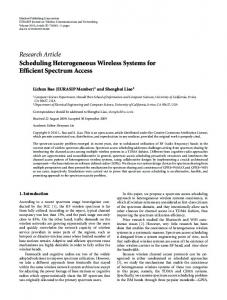
that SIGMOD and VLDB are similar, then SIGMOD authors and VLDB authors should be similar. Unfortunately, similarities between conferences may not be available, either. This problem can be solved by SimRank [12], in which the similarity between two objects is recursively defined as the average similarity between objects linked with them. For example, the similarity between two authors is the average similarity between the conferences in which they publish papers. In Figure 1 (b) “sigmod” and “vldb” have high similarity because they share many coauthors, and thus Tom and John become similar because they publish papers in similar conferences. In contrast, John and Mary do not have high similarity even they are both linked with “vldb05”. Although SimRank provides a good definition for similarities based on linkages, it is prohibitively expensive in computation. In [12] an iterative approach is proposed to compute the similarity between every pair of objects, which has quadratic complexity in both time and space, and is impractical for large databases. Is it necessary to compute and maintain pairwise similarities between objects? Our answer is no for the following two reasons. First, hierarchy structures naturally exist among objects of many types, such as the taxonomy of animals and hierarchical categories of merchandise. Consider the example of clustering authors according to their research. There are groups of authors working on the same research topic (e.g., data integration or XML), who have high similarity with each other. Multiple such groups may form a larger group, such as the authors working on the same research area (e.g., database vs. AI), who may have weaker similarity than the former. As a similar example, the density of linkages between clusters of articles and words is shown in Figure 2 (adapted from Figure 5 (b) in [4]). We highlight four dense regions with dashed boxes, and in each dense region there are multiple smaller and denser regions. The large dense regions correspond to high-level clusters, and the smaller denser regions correspond to low-level clusters within the high-level clusters.

portion of entries

0.4 0.3 0.2 0.1

0.24

0.2

0.22

0.18

0.16

0.14

0.1

0.12

0.08

0.06

0.04

0.02

0

0 similarity value

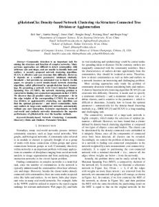
Figure 3: Portions of similarity values

Articles

design a data structure that stores the significant similarity values, and compresses those insignificant ones. Based on the above two observations, we propose a new hierarchical strategy to effectively prune the similarity space, which greatly speedups the identification of similar objects. Taking advantage of the power law distribution of linkages, we substantially reduce the number of pairwise similarities that need to be tracked, and the similarity between less similar objects will be approximated using aggregate measures. We propose a hierarchical data structure called SimTree as a compact representation of similarities between objects. Each leaf node of a SimTree corresponds to an object, and each non-leaf node contains a group of lower-level nodes that are closely related to each other. SimTree stores similarities in a multi-granularity way by storing similarity between each two objects corresponding to sibling leaf nodes, and storing the overall similarity between each two sibling nonleaf nodes. Pairwise similarity is not pre-computed or maintained between objects that are not siblings. Their similarity, if needed, is derived based on the similarity information stored in the tree path. For example, consider the hierarchical categories of merchandise in Walmart. It is meaningful to compute the similarity between every two cameras, but not so meaningful to compute that for each camera and each TV, as an overall similarity between cameras and TVs should be sufficient. Based on SimTree, we propose LinkClus, an efficient and accurate approach for linkage-based clustering. At the beginning LinkClus builds a SimTree for each type of objects in a bottom-up manner, by finding groups of objects (or groups of lower level nodes) that are similar to each other. Because inter-object similarity is not available yet, the similarity between two nodes are measured based on the intersection size of their neighbor objects. Thus the initial SimTrees cannot fully catch the relationships between objects (e.g., some SIGMOD authors and VLDB authors have similarity 0). LinkClus improves each SimTree with an iterative method, following the recursive rule that two nodes are similar if they are linked with similar objects. In each iteration it measures the similarity between two nodes in a SimTree by the average similarity between objects linked with them. For example, after one iteration SIGMOD and VLDB will become similar because they share many authors, which will then increase the similarities between SIGMOD authors and VLDB authors, and further increase that between SIGMOD and VLDB. We design an efficient algorithm for updating SimTrees, which merges the expensive similarity computations that go through the same paths in the SimTree. For a problem involving N objects and M linkages, LinkClus only takes O(M (log N )2 ) time and O(M + N ) space (SimRank takes O(M 2 ) time and O(N 2 ) space). Comprehensive experiments on both real and synthetic datasets are performed to test the accuracy and efficiency of

Words

Figure 2: Density of linkages between articles and words Second, recent studies show that there exist power law distributions among the linkages in many domains, such as Internet topology and social networks [8]. Interestingly, based on our observation, such relationships also exist in the similarities between objects in interlinked environments. For example, Figure 3 shows the distribution of pairwise SimRank similarity values between 4170 authors in DBLP database (the plot shows portion of values in each 0.005 range of similarity value). It can be seen that majority of similarity entries have very small values which lie within a small range (0.005 – 0.015). While only a small portion of similarity entries have significant values, — 1.4% of similarity entries (about 123K of them) are greater than 0.1, and these values will play the major role in clustering. Therefore, we want to

428

LinkClus. It is shown that the accuracy of LinkClus is either very close or sometimes even better than that of SimRank, but with much higher efficiency and scalability. LinkClus also achieves much higher accuracy than other approaches on linkage-based clustering such as ReCom [20], and approach for approximating SimRank with high efficiency [9]. The rest of the paper is organized as follows. We discuss related work in Section 2, and give an overview in Section 3. Section 4 introduces SimTree, the hierarchical structure for representing similarities. The algorithms for building SimTrees and computing similarities are described in Section 5. Our performance study is reported in Section 6, and this study is concluded in Section 7.

2.

challenging to identify the right pairs of objects at the beginning, because many pairs of similar objects can only be identified after computing similarities between other objects. In fact this is the major reason that we adopt the recursive definition of similarity and use iterative methods. A method is proposed in [9] to perform similarity searches by approximating SimRank similarities. It creates a large sample of random walk paths from each object and uses them to estimate the SimRank similarity between two objects when needed. It is suitable for answering similarity queries. However, very large samples of paths are needed for making accurate estimations for similarities. Thus it is very expensive in both time and space to use this approach for clustering a large number of objects, which requires computing similarities between numerous pairs of objects. Wang et al. propose ReCom [20], an approach for clustering inter-linked objects of different types. ReCom first generates clusters using attributes and linked objects of each object, and then repeatedly refines the clusters using the clusters linked with each object. Compared with SimRank that explores pairwise similarities between objects, ReCom only explores the neighbor clusters and does not compute similarities between objects. Thus it is much more efficient but much less accurate than SimRank. LinkClus is also related to hierarchical clustering [10, 17]. However, they are fundamentally different. Hierarchical clustering approaches use some similarity measures to put objects into hierarchies. While LinkClus uses hierarchical structures to represent similarities.

RELATED WORK

Clustering has been extensively studied for decades in different disciplines including statistics, pattern recognition, database, and data mining, with many approaches proposed [1, 10, 14, 15, 17, 22]. Most existing clustering approaches aim at grouping objects in a single table into clusters, using properties of each object. Some recent approaches [13, 21] extend previous clustering approaches to relational databases and measures similarity between objects based on the objects joinable with them in multiple relations. In many real applications of clustering, objects of different types are given, together with linkages among them. As the attributes of objects often provide very limited information, traditional clustering approaches can hardly be applied, and linkage-based clustering is needed, which is based on the principle that two objects are similar if they are linked with similar objects. This problem is related to bi-clustering [5] (or co-clustering [7], cross-association [4]), which aims at finding dense submatrices in the relationship matrix of two types of objects. A dense submatrix corresponds to two groups of objects of different types that are highly related to each other, such as a cluster of genes and a cluster of conditions that are highly related. Unlike bi-clustering that involves no similarity computation, LinkClus computes similarities between objects based on their linked objects. Moreover, LinkClus works on a more general problem as it can be applied to a relational database with arbitrary schema, instead of two types of linked objects. LinkClus also avoids the expensive matrix operations often used in bi-clustering approaches. A bi-clustering approach [7] is extended in [3], which performs agglomerative and conglomerative clustering simultaneously on different types of objects. However, it is very expensive, — quadratic complexity for two types and cubic complexity for more types. Jeh and Widom propose SimRank [12], a linkage-based approach for computing the similarity between objects, which is able to find the underlying similarities between objects through iterative computations. Unfortunately SimRank is very expensive as it has quadratic complexity in both time and space. The authors also discuss a pruning technique for approximating SimRank, which only computes the similarity between a small number of preselected object pairs. In the extended version of [12] the following heuristic is used: Only similarities between pairs of objects that are linked with same objects are computed. With this heuristic, in Figure 1 (b) the similarity between SIGMOD and VLDB will never be computed. Neither will the similarity between Tom and John, Tom and Mike, etc. In general, it is very

3.

OVERVIEW

Linkage-based clustering is based on the principle that two objects are similar if they are linked with similar objects. For example, in a publication database (Figure 1 (b)), two authors are similar if they publish similar papers. The final goal of linkage-based clustering is to divide objects into clusters using such similarities. Figure 4 shows an example of three types of linked objects, and clusters of similar objects which are inferred from the linkages. It is important to note that objects 12 and 18 do not share common neighbors, but they are linked to objects 22 and 24, which are similar because their common linkages to 35, 37 and 38. 11 12 13 14 15 16 17 18

21 22 23 24

31 32 33 34 35 36 37 38 39

17 14 15 11 13 12 18 16

23 21

22 24

33 39 34 36 31 37 32 35 38

Figure 4: Finding groups of similar objects In order to capture the inter-object relationships as in the above example, we adopt the recursive definition of similarity in SimRank [12], in which the similarity between two objects x and y is defined as the average similarity between the objects linked with x and those linked with y. As mentioned in the introduction, a hierarchical structure can capture the hierarchical relationships among objects, and can compress the majority of similarity values which are insignificant. Thus we use SimTree, a hierarchical structure for storing similarities in a multi-granularity way. It stores detailed similarities between closely related objects, and overall similarities between object groups. We

429

generalize the similarity measure in [12] to hierarchical environments, and propose an efficient and scalable algorithm for computing similarities based on the hierarchical structure. Each node in a SimTree has at most c children, where c is a constant and is usually between 10 and 20. Given a database containing two types of objects, N objects of each type, and M linkages between them, our algorithm takes O(N c + M ) space and O(M · (logc N )2 · c2 ) time. This is affordable for very large databases.

4.

SIMTREE: HIERARCHICAL REPRESENTATION OF SIMILARITIES

In this section we describe SimTree, a new hierarchical structure for representing similarities between objects. Each leaf node of a SimTree represents an object (by storing its ID), and each non-leaf node has a set of child nodes, which are a group of closely related nodes of one level lower. An example SimTree is shown in Figure 5 (a). The small gray circles represent leaf nodes, which must appear at the same level (which is level-0, the bottom level). The dashed circles represent non-leaf nodes. Each non-leaf node has at most c child nodes, where c is a small constant. Between each pair of sibling nodes ni and nj there is an undirected edge (ni , nj ). (ni , nj ) is associated with a real value s(ni , nj ), which is the average similarity between all objects linked with ni (or with its descendant objects if ni is a non-leaf node) and those with nj . s(ni , nj ) represents the overall similarity between the two groups of objects contained in ni and nj .

n1 0.8

n4 0.9

n7

a) Structure of a SimTree

0.3

n2

0.2

its parent. LinkClus makes some adjustments to compensate for such differences, by associating a value to the edge between each node and its parent. For example, the edge (n7 , n4 ) is associated with a real value s(n7 , n4 ), which is the ratio between (1) the average similarity between n7 and all leaf nodes except n4 ’s descendants, and (2) the average similarity between n4 and those nodes. Similarly we can define s(n4 , n1 ), s(n6 , n2 ), etc. When estimating the similarity between n7 and n9 , we use s(n1 , n2 ) as a basic estimation, use s(n4 , n1 ) to compensate for the difference between similarities involving n4 and those involving n1 , and use s(n7 , n4 ) to compensate for n7 . The final estimation is s(n7 , n4 ) · s(n4 , n1 ) · s(n1 , n2 ) · s(n6 , n2 ) · s(n9 , n6 )= 0.9 · 0.8 · 0.2 · 0.9 · 1.0 = 0.1296. In general, the similarity between two leaf nodes w.r.t. a SimTree is the product of the values of all edges on the path between them. Because this similarity is defined based on the path between two nodes, we call it path-based similarity. Definition 1. (Path-based Node Similarity) Suppose two leaf nodes n1 and nk in a SimTree are connected by path n1 → . . . → ni → ni+1 → . . . → nk , in which ni and ni+1 are siblings and all other edges are between nodes and their parents. The path-based similarity between n1 and nk is k−1 Y simp (n1 , nk ) = s(nj , nj+1 ) (1) j=1

Each node has similarity 1 with itself (simp (n, n) = 1). Please note that within a path in Definition 1, there is only one edge that is between two sibling nodes, whose similarity is used as the basic estimation. The other edges are between parent and child nodes whose similarities are used for adjustments.

n3

0.9

0.9

5.

n5

n6

The input to LinkClus are objects of different types, with linkages between them. LinkClus maintains a SimTree for each type of objects to represent similarities between them. Each object is used as a leaf node in a SimTree. Figure 6 shows the leaf nodes created from objects of two types, and the linkages between them.

0.8

n8

1.0

n9

b) Another view of the SimTree

Figure 5: An example SimTree Another view of the same SimTree is shown in Figure 5 (b), which better visualizes the hierarchical structure. The similarity between each pair of sibling leaf nodes is stored in the SimTree. While the similarity between two non-sibling leaf nodes is estimated using the similarity between their ancestor nodes. For example, suppose the similarity between n7 and n8 is needed, which is the average similarity between objects linked with n7 and those with n8 . One can see that n4 (or n5 ) contains a small group of leaf nodes including n7 (or n8 ), and we have computed s(n4 , n5 ) which is the average similarity between objects linked with these two groups of leaf nodes. Thus LinkClus uses s(n4 , n5 ) as the estimated similarity between n7 and n8 . In a real application such as clustering products in Walmart, n7 may correspond to a camera and n8 to a TV. We can estimate their similarity using the overall similarity between cameras and TVs, which may correspond to n4 and n5 , respectively. Similarly when the similarity between n7 and n9 is needed, LinkClus uses s(n1 , n2 ) as an estimation. Such estimation is not always accurate, because a node may have different similarities to other nodes compared with

BUILDING SIMTREES

10 11 12 13 14 15 16 17 18 19 20 21 22 23 24

l m n

o

p

q

r

s

t

u

v w x

y

ST2 ST1

Figure 6: Leaf nodes in two SimTrees Initially each object has similarity 1 to itself and 0 to others. LinkClus first builds SimTrees using the initial similarities. These SimTrees may not fully catch the real similarities between objects, because inter-object similarities are not considered. LinkClus uses an iterative method to improve the SimTrees, following the principle that two objects are similar if and only if they are linked with similar objects. It repeatedly updates each SimTree using the following rule: The similarity between two nodes ni and nj is the average similarity between objects linked with ni and those linked with nj . The structure of each SimTree is also adjusted during each iteration by moving similar nodes together. In this way the similarities are refined in each iteration, and the relationships between objects can be discovered gradually.

430

Nodes g1

n1 n2

g2

n3 n4

the group with highest support that is not overlapped with l previously selected groups. After selecting αN groups, we c create a level-(l + 1) node based on each group. However, these groups usually cover only part of all level-l nodes. For each level-l node ni that does not belong to any group, we want to put ni into the group that is most connected with ni . For each group g, we compute the number of objects that are linked with both ni and some members of g, which is used to measure the connection between ni and g. We assign ni to the group with highest connection to ni .

Transactions 1 2 3 4 5 6 7 8 9

{n1} {n1, n2} {n2} {n1, n2} {n2} {n2, n3, n4} {n4} {n3, n4} {n3, n4}

Figure 7: Groups of tightly related nodes

5.1

Initializing SimTrees Using Frequent Pattern Mining

Level 2

The first step of LinkClus is to initialize SimTrees using the linkages as shown in Figure 6. Although no inter-object similarities are available at this time, the initial SimTrees should still be able to group related objects or nodes together, in order to provide a good base for further improvements. Because only leaf nodes are available at the beginning, we initialize SimTrees from bottom level to top level. At each level, we need to efficiently find groups of tightly related nodes, and use each group as a node of the upper level. Consider a group of nodes g = {n1 , . . . , nk }. Let neighbor(ni ) denote the set of objects linked with node ni . Initially there are no inter-object similarities, and whether two nodes are similar depends on whether they are co-linked with many objects. Therefore, we define the tightness of group g as the number of objects that are linked with all group members, i.e., the size of intersection of neighbor(n1 ), . . . , neighbor(nk ). The problem of finding groups of nodes with high tightness can be reduced to the problem of finding frequent patterns [2]. A tight group is a set of nodes that are co-linked with many objects of other types, just like a frequent pattern is a set of items that co-appear in many transactions. Figure 7 shows an example which contains four nodes n1 , n2 , n3 , n4 and objects linked with them. The nodes linked with each object are converted into a transaction, which is shown on the right side. It can be easily proved that, the number of objects that are linked with all members of a group g is equal to the support of the pattern corresponding to g in the transactions. For example, nodes n1 and n2 are co-linked with two objects (#2 and #4), and pattern {n1 , n2 } has support 2 (i.e., appear twice) in the transactions. Let support(g) represent the number of objects linked with all nodes in g. When building a SimTree, we want to find groups with high support and at least min size nodes. For two groups g and g ′ such that g ⊂ g ′ and support(g) = support(g ′ ), we prefer g ′ . Frequent pattern mining has been studied for a decade with many efficient algorithms. We can either find groups of nodes with support greater than a threshold using a frequent closed pattern mining approach [19], or find groups with highest support using a top-k frequent closed pattern mining approach [11]. LinkClus uses the approach in [19] which is very efficient on large datasets. Now we describe the procedure of initializing a SimTree. Suppose we have built Nl nodes at level-l of the SimTree, and want to build the nodes of level-(l + 1). Because each node can have at most c child nodes, and because we want to leave some space for further adjustment of the tree structure, we control the number of level-(l + 1) nodes to be between Nl l and αN (1 < α ≤ 2). We first find groups of level-l c c nodes with sufficiently high support. Since there are usually l non-overlapping groups many such groups, we select αN c with high support in a greedy way, by repeatedly selecting

Level 1

ST2

0

Level 3

1 4

2 5

3

6

7

8

9

Level 0

10 11 12 13 14 15 16 17 18 19 20 21 22 23 24

Level 3

z

ST1

d

e

Level 2

c

Level 1

a

b

f

Level 0

l m n

o p

q r

g s

h t

u v w

k x

y

Figure 8: Some linkages between two SimTrees Figure 8 shows the two SimTrees built upon the leaf nodes in Figure 6. The dashed lines indicate the leaf nodes in ST2 that are linked with descendants of two non-leaf nodes na and nb in ST1 . After building the initial SimTrees, LinkClus computes the similarity value associated with each edge in the SimTrees. As defined in Section 4, the similarity value of edge (na , nb ), s(na , nb ), is the average similarity between objects linked with descendants of na and those of nb . Because initially the similarity between any two different objects is 0, s(na , nb ) can be easily computed based on the number of objects that are linked with both the descendants of na and those of nb , without considering pairwise similarities. Similarly, the values associated with edges between child and parent nodes can also be computed easily.

5.2

Refining Similarity between Nodes

The initial SimTrees cannot fully catch the real similarities, because similarities between objects are not considered when building them. Therefore, LinkClus repeatedly updates the SimTrees, following the principle that the similarity between two nodes in a SimTree is the average similarity between the objects linked with them, which is indicated by other SimTrees. This is formally defined in this subsection. We use [n ∼ n′ ] to denote the linkage between two nodes n and n′ in different SimTrees. We say there is a linkage between a non-leaf node n in ST1 and a node n′ in ST2 , if there are linkages between the descendant leaf nodes of n and the node n′ . Figure 8 shows the linkages between na , nb and leaf nodes in ST2 . In order to track the number of original linkages involved in similarity computation, we assign a weight to each linkage. By default the weight of each original linkage between two leaf nodes is 1. The weight of linkage [n ∼ n′ ] is the total number of linkages between the descendant leaf nodes of n and n′ . In each iteration LinkClus updates the similarity between each pair of sibling nodes (e.g., na and nb ) in each SimTree, using the similarities between the objects linked with them in other SimTrees. The similarity between na and nb is the average path-based similarity between the leaf nodes linked with na ({n10 ,n11 ,n12 ,n16 }) and those with nb ({n10 ,n13 ,n14 , n17 }). Because this similarity is based on linked objects, we

431

Example 1. A simplified version of Figure 8 is shown in Figure 9, where siml (na , nb ) is the average path-based similarity between each node in {n10 ,n11 ,n12 } and each in {n13 ,n14 }. For each node nk ∈ {n10 ,n11 ,n12 } and nl ∈ {n13 ,n14 }, their path-based similarity simp (nk , nl ) = s(nk , n4 )· s(n4 , n5 ) · s(n5 , nl ). All these six path-based similarities involve s(n4 , n5 ). Thus siml (na , nb ), which is the average of them, can be written as

call it linkage-based similarity. na (or nb ) may have multiple linkages to a leaf node ni in ST2 , if more than one descendants of na are linked with ni . Thus the leaf nodes in ST2 linked with na are actually a multi-set, and the frequency of each leaf node ni is weight([na ∼ ni ]), which is the number of original linkages between na and ni . The linkage-based similarity between na and nb is defined as the average pathbased similarity between these two multi-sets of leaf nodes, and in this way each original linkage plays an equal role.

siml (na , nb ) =

Definition 2. (Linkage-based Node Similarity) Suppose a SimTree ST is linked with SimTrees ST1 , . . . , STK . For a node n in ST , let N BSTk (n) denote the multi-set of leaf nodes in STk linked with n. Let wn′ n′′ represent weight([n′ ∼ n′′ ]). For two nodes na and nb in ST , their linkage-based similarity siml (na , nb ) is the average similarity between the multi-set of leaf nodes linked with na and that of nb . We decompose the definition into several parts for clarity. (The total weights between N BSTk (na ) and N BSTk (nb )) X X weightSTk (na , nb ) = wna n · wnb n′ n∈N BST (na ) n′ ∈N BST (nb ) k

k

(The sum of weighted similarity between them) X X sumSTk (na , nb ) = wna n ·wnb n′ ·simp (n, n′ ) n∈N BST (na ) n′ ∈N BST (nb ) k

k

(The linkage-based similarity between na and nb w.r.t. STk ) simSTk (na , nb ) =

sumSTk (na , nb ) weightSTk (na , nb )

(The final definition of siml (na , nb )) K 1 X siml (na , nb ) = simSTk (na , nb ). K k=1

(2)

Equation (2) shows that if a SimTree ST is linked with multiple SimTrees, each linked SimTree plays an equal role in determining the similarity between nodes in ST . The user can also use different weights for different SimTrees according to the semantics.

5.3

Aggregation-based Similarity Computation

The core part of LinkClus is how to iteratively update each SimTree, by computing linkage-based similarities between different nodes. This is also the most computation-intensive part in linkage-based clustering. Definition 2 provides a brute-force method to compute linkage-based similarities. However, it is very expensive. Suppose each of two nodes na and nb is linked with m leaf nodes. It takes O(m2 logc N ) to compute siml (na , nb ) (logc N is the height of SimTree). Because some high-level nodes are linked with Θ(N ) objects, this brute-force method requires O(N 2 logc N ) time, which is unaffordable for large databases. Fortunately, we find that the computation of different path-based similarities can be merged if these paths are overlapped with each other. The two numbers in a bracket represent the average similarity and total weight of a linkage between two nodes

a:(0.9,3)

0.2

4 0.9 10

a:(1,1)

1.0 0.8 11

12

a:(1,1) a:(1,1)

a

1.0

13

14

b:(1,1)

b:(1,1)

b

s(nk , n4 ) · s(n4 , n5 ) · 3

P 14

l=13

s(nl , n5 ) . 2 (3)

Equation (3) contains three parts: the average similarity between na and descendants of n4 , s(n4 , n5 ), and the average similarity between nb and descendants of n5 . Therefore, we pre-compute the average similarity and total weights between na ,nb and n4 ,n5 , as shown in Figure 9. (The original linkages between leaf nodes do not affect similarities and thus have similarity 1.) We can compute siml (na , nb ) using such × 0.2 × 0.9+1.0 = aggregates, i.e., siml (na , nb ) = 0.9+1.0+0.8 3 2 0.9 × 0.2 × 0.95 = 0.171, and this is the average similarity between 3 × 2 = 6 pairs of leaf nodes. This is exactly the same as applying Definition 2 directly. But now we have avoided the pairwise similarity computation, since only the edges between siblings and parent-child are involved. This mini example shows the basic idea of computing linkage-based similarities. In a real problem na and nb are often linked with many leaf nodes lying in many different branches of the SimTrees, which makes the computation much more complicated. The basic idea is still to merge computations that share common paths in SimTrees. To facilitate our discussion, we introduce a simple data type called simweight, which is used to represent the similarity and weight associated with a linkage. A simweight is a pair of real numbers hs, wi, in which s is the similarity of a linkage and w is its weight. We define two operations of simweight that are very useful in LinkClus. Definition 3. (Operations of simweight) The operation of addition is used to combine two simweights corresponding to two linkages. The new similarity is the weighted average of their similarities, and the new weight is the sum of their weights: s1 · w1 + s2 · w2 , w1 + w2 i. (4) hs1 , w1 i + hs2 , w2 i = h w1 + w2

Lemma 1. The laws of commutation, association, and distribution hold for the operations of simweight. LinkClus uses a simweight to represent the relationship between two nodes in different SimTrees. We use N BST (n) to denote the multi-set of leaf nodes in ST linked with node n. For example, in Figure 8 N BST2 (na ) ={n10 ,n11 ,n12 ,n16 } and N BST2 (nb ) = {n10 ,n13 ,n14 ,n17 }. We first define the weight and similarity of a linkage between two non-leaf nodes in two SimTrees. A non-leaf node represents the set of its child nodes. Therefore, for a node na in ST1 and a non-leaf node ni in ST2 , the weight and similarity of linkage [na ∼ ni ] is the sum of weights and weighted average similarity between their child nodes. Furthermore, according to Definition 1, the similarity between two non-sibling nodes ni and nj on the same level of ST2 can be calculated as

ST2

5

k=10

The operation of multiplication is used to compute the weighted average similarity between two sets of leaf nodes. The new weight w1 · w2 represents the number of pairs of leaf nodes between the two sets. hs1 , w1 i × hs2 , w2 i = hs1 · s2 , w1 · w2 i. (5)

b:(0.95,2) 0.9

P 12

ST1

Figure 9: Computing similarity between nodes

432

a:(0.9,3) b:(0.9,1)

0.9 a:(1,1) b:(1,1) 10

a:(0.81,3) b:(0.903,3)

4 11

0.8 a:(1,1)

2

1.0 0.2

1.0 0.4

0.1

1

0.9

12

a:(1,1)

0.9

5 0.9

Theorem 1. (Sibling-pair based Similarity Computation) Suppose na and nb are two nodes in SimTree ST1 . Let N BST2 (na ) and N BST2 (nb ) be the multi-sets of leaf nodes in SimTree ST2 linked with na and nb , respectively.

ST2

0

simweights of linkage [na~n1] and [nb~n1]

6

b:(0.95,2)

0.9

1.0

13 b:(1,1) 14 b:(1,1)

a:(1,1)

a:(0.81,1) b:(0.9,1) a:(0.9,1) b:(1.0,1)

1.0

hsiml (na , nb ), weight is ignoredi = X X swna ni × hs(ni , nj ), 1i × swnb nj

16 0.5 17 b:(1,1)

0.3

n∈ST2 ni ,nj ∈children(n),ni 6=nj

a

b

ST1

+

Figure 10: Computing similarity between nodes

X

ni ∈N BST2 (na )

simp (ni , nj ) = s(ni , parent(ni )) · simp (parent(ni ), parent(nj )) · s(nj , parent(nj )).

Thus we also incorporate s(ni , parent(ni )) (i.e., the ratio between average similarity involving ni and that involving parent(ni )) into the definition of linkage [na ∼ ni ]. We use swna ni to denote the simweight of [na ∼ ni ]. Definition 4. Let na be a node in SimTree ST1 and ni be a non-leaf node in ST2 . Let children(ni ) be all child nodes of ni . The simweight of linkage [na ∼ ni ] is defined as X swna ni = hs(ˆ n, ni ), 1i × swna nˆ . (6) n ˆ ∈children(ni )

(In Equation (6) we use hx, 1i × hs, wi as a convenient notation for hx · s, wi. Figure 9 and Figure 10 show swna ni and swnb ni for each node ni in ST2 .) Using Definition 4, we formalize the idea in Example 1 as follows. Lemma 2. For two nodes na and nb in SimTree ST1 , and two sibling non-leaf nodes ni and nj in ST2 , the average similarity and total weight between the descendant objects of ni linked with na and those of nj linked with nb is swna ni × hs(ni , nj ), 1i × swnb nj . (This corresponds to Equation (3) if i = 4 and j = 5.)

We outline the procedure for computing the linkage-based similarity between na and nb (see Figure 10). siml (na , nb ) is the average similarity between N BST2 (na ) and N BST2 (nb ). We first compute the aggregated simweights swna n and swnb n for each node n in ST2 , if n is an ancestor of any node in N BST2 (na ) or N BST2 (nb ), as shown in Figure 10. Consider each pair of sibling nodes ni and nj in ST2 (e.g., n4 and n5 ), so that ni is linked with na and nj with nb . According to Lemma 1, the average similarity and total weight between the descendant objects of ni linked with na and those of nj linked with nb is swna ni × hs(ni , nj ), 1i × swnb nj . For example, swna n4 = h0.9, 3i (where the weight is 3 as na can reach n4 via n10 , n11 or n12 ), swnb n5 = h0.95, 2i, and s(n4 , n5 ) = 0.2. Thus swna n4 × hs(n4 , n5 ), 1i × swnb n5 = h0.171, 6i (as in Example 1), which represents the average similarity and total weights between {n10 ,n11 ,n12 } and {n13 ,n14 }. We note that the weight is 6 as there are 6 paths between leaf nodes under n4 linked with na and those under n5 linked with nb . From the above example it can be seen that the effect of similarity between every pair leaf nodes in ST2 will be captured when evaluating their ancestors that are siblings. For any two leaf nodes n ˆ i and n ˆ j in ST2 , there is only one ancestor of n ˆ i and one of n ˆ j that are siblings. Thus every pair of n ˆi, n ˆ j (ˆ ni ∈ N BST2 (na ), n ˆ j ∈ N BST2 (nb )) is counted exactly once, and no redundant computation is performed. In general, siml (na , nb ) can be computed using Theorem 1.

T

swna ni × swnb ni .

(7)

N BST2 (nb )

The first term of equation (7) corresponds to similarities between different leaf nodes. For all leaf nodes under ni linked with na and those under nj linked with nb , the effect of pairwise similarities between them is aggregated together as computed in the first term. The second term of equation (7) corresponds to the leaf nodes linked with both na and nb . Only similarities between sibling nodes are used in equation (7), and thus we avoid the tedious pairwise similarity computation in Definition 2. In order to compute the linkagebased similarities between nodes in ST1 , it is sufficient to compute aggregated similarities and weights between nodes in ST1 and nodes in other SimTrees. This is highly efficient in time and space as shown in Section 5.5. Now we describe the procedure of computing siml (na , nb ) based on Theorem 1. Step 1: Attach the simweight of each original linkage involving descendants of na or nb to the leaf nodes in ST2 . Step 2: Visit all leaf nodes in ST2 that are linked with both na and nb to compute the second term in Equation (7). Step 3: Aggregate the simweights on the leaf nodes to those nodes on level-1. Then further aggregate simweights to nodes on level-2, and so on. Step 4: For each node ni in ST2 linked with na , and each sibling of ni that is linked with nb (we call it nj ), add swna ni × hs(ni , nj ), 1i × swnb nj to the first term of equation (7). Suppose na is linked with m leaf nodes in ST2 , and nb is linked with O(m · c) ones. It is easy to verify that the above procedure takes O(mc logc N ) time.

5.4

Iterative Adjustment of SimTrees

After building the initial SimTrees as described in Section 5.1, LinkClus needs to iteratively adjust both the similarities and structure of each SimTree. In Section 5.3 we have described how to compute the similarity between two nodes using similarities between their neighbor leaf nodes in other SimTrees. In this section we will introduce how to restructure a SimTree so that similar nodes are put together. The structure of a SimTree is represented by the parentchild relationships, and such relationships may need to be modified in each iteration because of the modified similarities. In each iteration, for each node n, LinkClus computes n’s linkage-based similarity with parent(n) and the siblings of parent(n). If n has higher similarity with a sibling node n ˇ of parent(n), then n will become a child of n ˇ , if n ˇ has less than c children. The moves of low-level nodes can be considered as local adjustments on the relationships between objects, and the moves of high-levels nodes as global adjustments on the relationships between large groups of objects. Although each node can only be moved within a small range (i.e., its parent’s siblings), with the effect of both local and

433

Algorithm 1. Restructure SimTree

updates the values associated with edges in each SimTree. When restructuring ST1 , for each node n in ST1 , LinkClus needs to compute its similarity to its parent and parent’s siblings, which are at most c nodes. Suppose n is linked with m leaf nodes in ST2 . As shown in Section 5.3, it takes O(mc logc N ) time to compute the n’s similarity with its parent or each of its parent’s siblings. Thus it takes O(mc2 logc N ) time to compute the similarities between n and these nodes. There are N leaf nodes in ST1 , which have a total of M linkages to all leaf nodes in ST2 . In fact all nodes on each level in ST1 have M linkages to all leaf nodes in ST2 , and there are O(logc N ) levels. Thus it takes O(M c2 (logc N )2 ) time in total to compute the similarities between every node in ST1 and its parent and parent’s siblings. In the above procedure, LinkClus processes nodes in ST1 level by level. When processing the leaf nodes, only the simweights of linkages involving leaf nodes and nodes on level-1 of ST1 are attached to nodes in ST2 . There are O(M ) such linkages, and the simweights on the leaf nodes in ST2 require O(M ) space. In ST2 LinkClus only compares the simweights of sibling nodes, thus it can also process the nodes level by level. Therefore, the above procedure can be done in O(M ) space. Each SimTree has O(N ) nodes, and it takes O(c) space to store the similarity between each node and its siblings (and its parent’s siblings). Thus the space requirement is O(M + N c). It can be easily shown that the procedure for restructuring a SimTree (Algorithm 1) takes O(N c) space and O(N c log c) time, which is much faster than computing similarities. After restructuring SimTrees, LinkClus computes the similarities between each node and its siblings. This can be done using the same procedure as computing similarities between each node and its parent’s siblings. Therefore, each iteration of LinkClus takes O(M c2 (logc N )2 ) time and O(M +N c) space. This is affordable for very large databases.

Input: a SimTree ST to be restructured, which is linked with SimTrees ST1 , . . . , STk . Output: The restructured ST . Sc ← all nodes in ST except root //Sc contains all child nodes Sp ← all non-leaf nodes in ST //Sp contains all parent nodes for each node n in Sc //find most similar parent node for n for each sibling node n′ of parent(n) (including parent(n)) compute siml (n, n′ ) using ST1 , . . . , STk sort the set of siml (n, n′ ) for n p∗ (n) ← n′ with maximum siml (n, n′ ) while(Sc 6= ∅) for each node n ˇ ∈ Sp //assign children to n ˇ q ∗ (ˇ n) ← {n|p∗ (n) = n ˇ} if |q ∗ (ˇ n)| < c then children(ˇ n) ← q ∗ (ˇ n) else children(ˇ n) ← c nodes in q ∗ (ˇ n) most similar to n ˇ Sp ← Sp − {ˇ n} Sc ← Sc − children(ˇ n) for each node n ∈ Sc p∗ (n) ← n′ with maximum siml (n, n′ ) and n′ ∈ Sp return ST

Figure 11: Algorithm Restructure SimTree global adjustments, the tree restructure is often changed significantly in an iteration. The procedure for restructuring a SimTree is shown in Algorithm 1. LinkClus tries to move each node n to be the child of a parent node that is most similar to n. Because each non-leaf node n ˇ can have at most c children, if there are more than c nodes that are most similar to n ˇ , only the top c of them can become children of n ˇ , and the remaining ones are reassigned to be children of other nodes similar to them. After restructuring a SimTree ST , LinkClus needs to compute the value associated with every edge in ST . For each edge between two sibling nodes, their similarity is directly computed as in Section 5.3. For each edge between a node n and its parent, LinkClus needs to compute the average similarity between n and all leaf nodes except descendants of parent(n), and that for parent(n). It can be proved that the average linkage-based similarity between n and all leaf nodes in ST except descendants of a non-leaf node n′ is sumSTk (n, root(ST )) − sumSTk (n, n′ )) (8) weightSTk (n, root(ST )) − weightSTk (n, n′ ))

6.

Please note that equation (8) uses notations in Definition 2. With equation (8) we can compute the similarity ratio associated with each edge between a node and its parent. This finishes the computation of the restructured SimTree.

5.5

EMPIRICAL STUDY

In this section we report experiments to examine the efficiency and effectiveness of LinkClus. LinkClus is compared with the following approaches: (1) SimRank [12], an approach that iteratively computes pairwise similarities between objects; (2) ReCom [20], an approach that iteratively clusters objects using the cluster labels of linked objects; (3) SimRank with fingerprints [9] (we call it F-SimRank ), an approach that pre-computes a large sample of random paths from each object and uses the samples of two objects to estimate their SimRank similarity; (4) SimRank with pruning (we call it P-SimRank ) [12], an approach that approximates SimRank by only computing similarities between pairs of objects reachable within a few links. SimRank and F-SimRank are implemented strictly following their papers. (We use decay factor 0.8 for F-SimRank, which leads to highest accuracy in DBLP database.) ReCom is originally designed for handling web queries, and contains a reinforcement clustering approach and a method for determining authoritativeness of objects. We only implement the reinforcement clustering method, because it may not be appropriate to consider authoritativeness in clustering. Since SimRank, F-SimRank and P-SimRank only provide similarities between objects, we use CLARANS [15], a k-medoids clustering approach, for clustering using such similarities. CLARANS is also used in ReCom since no specific cluster-

Complexity Analysis

In this section we analyze the time and space complexity of LinkClus. For simplicity, we assume there are two object types, each having N objects, and there are M linkages between them. Two SimTrees ST1 and ST2 are built for them. If there are more object types, the similarity computation between each pair of linked types can be done separately. When a SimTree is built, LinkClus limits the number of nodes at each level. Suppose there are Nl nodes on levell. The number of nodes on level-(l + 1) must be between Nl l and αN (α ∈ [1, 2] and usually c ∈ [10, 20]). Thus the c c height of a SimTree is O(logc N ). In each iteration, LinkClus restructures each SimTree using similarities between nodes in the other SimTree, and then

434

paper-id title proc-id

Has-Keyword paper-id keyword-id

Conferences conference publisher

Figure 12: The schema of the DBLP database

Evaluation Measures

ics, networking, security, HCI, software engineering, information retrieval, bioinformatics, and CAD. For each conference, we study its historical call for papers to decide its area. 90% of conferences are associated with a single area. The other 10% are associated with multiple areas, such as KDD (database and AI). We analyze the research areas of 400 most productive authors. For each of them, we find her home page and infer her research areas from her research interests. If no research interests are specified, we infer her research areas from her publications. On average each author is interested in 2.15 areas. In the experiments each type of objects are grouped into 20 clusters, and the accuracy is tested based on the class labels. We first perform experiments without keywords. 20 iterations are used for SimRank, P-SimRank, ReCom, and LinkClus2 (not including the initialization process of each approach). In F-SimRank we draw a sample of 100 paths (as in [9]) of length 20 for each object, so that F-SimRank can use comparable information as SimRank with 20 iterations. The accuracies of clustering authors and conferences of each approach are shown in Figure 13 (a) and (b), in which the x-axis is the index of iterations.

Validating clustering results is crucial for evaluating approaches. In our test databases there are predefined class labels for certain types of objects, which are consistent with our clustering goals. Jaccard coefficient [18] is a popular measure for evaluating clustering results, which is the number of pairs of objects in same cluster and with same class label, over that of pairs of objects either in same cluster or with same class label. Because an object in our databases may have multiple class labels but can only appear in one cluster, there may be many more pairs of objects with same class label than those in same cluster. Therefore we use a variant of Jaccard coefficient. We say two objects are correctly clustered if they share at least one common class label. The accuracy of clustering is defined as the number of object pairs that are correctly clustered over that of object pairs in same cluster. Higher accuracy tends to be achieved when number of clusters is larger. Thus we let each approach generate the same number of clusters.

DBLP Database

We first test on the DBLP database, whose schema is shown in Figure 12. It is extracted from the XML data of DBLP [6]. We want to focus our analysis on the productive authors and well-known conferences1 , and group them into clusters so that each cluster of authors (or conferences) are in a certain research area. We first select conferences that have been held for at least 8 times. Then we remove conferences that are not about computer science or are not well known, and there are 154 conferences left. We select 4170 most productive authors in those conferences, each having at least 12 publications. The P ublications relation contains all publications of the selected authors in the selected conferences. We select about 2500 most frequent words (stemmed) in titles of the publications, except 50 most frequent words which are removed as stop words. There are four types of objects to be clustered: 4170 authors, 2517 proceedings, 154 conferences, and 2518 keywords. Publications are not clustered because too limited information is known for them (about 65% of publications are associated with only one selected author). There are about 100K linkages between authors and proceedings, 363K linkages between keywords and authors, and 363K between keywords and proceedings. Because we focus on clustering with linkages instead of keywords, we perform experiments both with and without the keywords. We manually label the areas of the most productive authors and conferences to measure clustering accuracy. The following 14 areas are considered: Theory, AI, operating system, database, architecture, programming languages, graph-

1

0.8 0.7

accuracy

0.6

0.9 LinkClus SimRank ReCom F-SimRank

0.85

0.4

LinkClus SimRank ReCom F-SimRank

0.3 0.2

#iteration

a) DBLP.Authors

19

15

17

11

13

7

9

3

5

19

17

15

13

9

11

0.1

7

1

0.8

0.5

1

accuracy

0.95

5

6.2

Proceedings proc-id conference year location

Publications

author-id paper-id

Keywords keyword-id keyword

3

6.1

Publishes

Authors author-id author-name

ing method is discussed in [20]. We compare LinkClus using both hierarchical clustering and CLARANS. All experiments are performed on an Intel PC with a 3.0GHz P4 processor, 1GB memory, running Windows XP Professional. All approaches are implemented √ using Visual Studio.Net (C#). In LinkClus, α is set to 2. We will discuss the influences of c (max number of children of each node) on accuracy and efficiency in the experiments.

#iteration

b) DBLP.Conferences

Figure 13: Accuracy on DBLP w/o keywords From Figure 13 one can see that SimRank is most accurate, and LinkClus achieves similar accuracy as SimRank. The accuracies of ReCom and F-SimRank are significantly lower. The error rates (i.e., 1 – accuracy) of ReCom and F-SimRank are about twice those of SimRank and LinkClus on authors, and 1.5 times those of them on conferences. One interesting observation is that more iterations do not necessarily lead to higher accuracy. This is probably because cluster labels are not 100% coherent with data. In fact this is common for iterative clustering algorithms. In the above experiment, LinkClus generates 20 clusters directly from the SimTrees: Given a SimTree, it first finds the level in which the number of nodes is most close to 20. Then it either keeps merging the most similar nodes if the number of nodes is more than 20, or keeps splitting the node

1 Here conferences refer to conferences, journals and workshops. We are only interested in productive authors and well-known conferences because it is easier to determine the research fields related to each of them, from which the accuracy of clustering will be judged.

2 Since no frequent patterns of conferences can be found using the proceedings linked to them, LinkClus uses authors linked with conferences to find frequent patterns of conferences, in order to build the initial SimTree for conferences.

435

Time/iteration

trade-off between accuracy and efficiency. This trade-off is shown in Figure 15, which contains the “accuracy vs. time” plots of SimRank, ReCom, LinkClus with different c’s (8 to 22, including c = 16 with CLARANS), and F-SimRank with sample size of 50, 100, 200 and 400. It also includes SimRank with pruning (P-SimRank), which uses the following pruning method: For each object x, we only compute its similarity with the top-k objects that share most common neighbors with x within two links (k varies from 100 to 500). In these two plots, the approaches in the top-left region are good ones as they have high accuracy and low running time. It can be clearly seen that LinkClus greatly outperforms the other approaches, often in both accuracy and efficiency. In comparison, pruning technique of SimRank does not improve much on efficiency, because it requires using hashtables to store similarities, and an access to a hashtable is 5 to 10 times slower than that to a simple array.

76.74 sec 107.7 sec 1020 sec 43.1 sec 83.6 sec

Table 1: Performances on DBLP without keywords with most descendant objects if otherwise, until 20 nodes are created. We also test LinkClus using CLARANS with the similarities indicated by SimTrees. The max accuracies and running time of different approaches are shown in Table 1. (The running time per iteration of F-SimRank is its total running time divided by 20.) One can see that the accuracy of LinkClus with CLARANS is slightly higher than that of LinkClus, and is close to that of SimRank. While SimRank is much more time consuming than other approaches.

1

0.7

8

11

16

22 C

32

45

128

a) Max accuracy

128

LinkClus LinkClus-Clarans SimRank ReCom F-SimRank

0

500

1000 Time (sec)

a) DBLP.Authors

1500

Accuracy

Accuracy

0.8

0.6 LinkClus SimRank ReCom F-SimRank P-SimRank

0.4 0

500

1000 Time (sec)

accuracy

7

9

3

5

Max accuracy Authors Conferences 0.9412 0.7743 0.9342 0.7287 0.9663 0.7953 0.9363 0.5447 0.6742 0.3032

Time/iteration 614.0 sec 654.9 sec 25348 sec 101.2 sec 136.3 sec

Table 2: Performances on DBLP with keywords Table 2 shows the max accuracy and running time of each approach. The total number of linkages grows about 8 times when keywords are used. The running time of LinkClus grows linearly, and that of SimRank grows quadratically. Because ReCom considers linked clusters of each object, instead of linked objects, its running time does not increase too much. The running time of F-SimRank does not increase much as it uses the same number of random paths. We also test LinkClus with different c’s, as shown in Figure 17. The accuracy is highest when c = 16 or 22. Figure 18 shows the curves of accuracies vs. running time (in log scale) of LinkClus, SimRank, ReCom, F-SimRank, and P-SimRank (100 to 400 similarity entries for each object). One can see that LinkClus is the most competitive method, as it achieves high accuracies and is 40 times more efficient than SimRank.

0.7

0.5

#iteration

b) DBLP.Conferences

Figure 16: Accuracy on DBLP with keywords Then we test on the DBLP database with keyword information. The accuracies of the approaches on authors and conferences are shown in Figure 16 (a) and (b). We only finish 7 iterations for SimRank because it is too time consuming. When using keywords, the accuracies of most approaches either increase or remain the same. The only exception is F-SimRank, whose accuracy drops more than 20%. This is because there are many more linkages when keywords are used, but F-SimRank still uses the same sample size, which makes the samples much sparser.

0.96

0.84

1

#iteration

0.8

LinkClus SimRank ReCom F-SimRank P-SimRank

0

a) DBLP.Authors

b) Running time

1

0.88

LinkClus SimRank ReCom F-SimRank

0.2

11

45

Figure 14: LinkClus with different c’s In the above experiments we use c = 16 for LinkClus. c is an important parameter for LinkClus, and thus we analyze its influences on accuracy and running time. As shown√in Figure 14, we test c from 8 to 45, each differing by 2. The running time grows almost linearly, and the accuracy is highest when c equals 16 and 22. Theoretically, more similarities are computed and stored as c increases, and the accuracy should also increase (LinkClus becomes SimRank when c is larger than the number of objects). However, when c increases from 16 to 45, the SimTrees of authors and proceedings always have four levels, and that of conferences has three levels. Although more similarities are stored at lower levels of the SimTrees, there are a comparatively small number of nodes at the second highest level. Thus not much more information is stored when c increases from 16 to 45. On the other hand, it may be difficult to generate 20 clusters if the second highest level has too few nodes. In comparison, when c = 128 the SimTrees have less levels, and accuracies become higher. Figure 14 also shows that the initialization time of LinkClus is very insignificant.

0.92

0.3

13

32

17

22 C

19

16

13

11

15

8

9

1

0.4

0.4

0.1

0.6

1

11

0.5

0.7

0.5

19

10

LinkClus-Author LinkClus-Conf SimRank-Author SimRank-Conf

LinkClus SimRank ReCom F-SimRank

0.8

7

0.6

0.6

100 accuracy

0.7

0.9

15

Initialization time/20

Seconds

Accuracy

0.9 0.8

0.8

Time/iteration

17

1000

3

1

5

LinkClus LinkClus-Clarans SimRank ReCom F-SimRank

Max accuracy Authors Conferences 0.9574 0.7229 0.9529 0.7523 0.9583 0.7603 0.9073 0.4567 0.9076 0.5829

1500

b) DBLP.Conferences

Figure 15: Accuracy vs. Time on DBLP w/o keywords In many methods of linkage-based clustering there is a

436

10000

procedure for x · w times: Randomly select an object o in Ri , and find the two clusters in Ri%4+1 associated with the cluster of o. Then generate a linkage between o and a randomly selected object in these two clusters with probability (1 − noise ratio), and generate a linkage between o and a randomly selected object with probability noise ratio. The default value of noise ratio is 20%. It is shown in previous experiments that in most cases each approach can achieve almost the highest accuracy in 10 iterations, we use 10 iterations in this subsection. We let each approach generate z clusters for a database RxT yCzSw. For LinkClus we use c = 16 and do not use CLARANS.

Time/iteration 0.9

Initialization time/20

Seconds

Accuracy

1000 0.8 0.7 0.6

100

LinkClus-Author LinkClus-Conf SimRank-Author SimRank-Conf

0.5 0.4 8

11

16

22 C

32

45

10 1 8

128

a) Max accuracy

11

16

22 C

32

45

128

b) Running time

Figure 17: LinkClus with different c’s 1

0.8

0.8 LinkClus SimRank ReCom F-SimRank P-SimRank

0.7

Accuracy

Accuracy

0.9

R1

0.6

R8

0.4

R4 LinkClus SimRank ReCom F-SimRank P-SimRank

0.2

0

0.6 10

100

1000 Time (sec)

10000

100000

a) DBLP.Authors

10

100

1000 Time (sec)

10000

100000

b) DBLP.Conferences

Email Dataset

LinkClus SimRank ReCom F-SimRank CLARANS

LinkClus SimRank ReCom F-SimRank O(N) O(N*(logN)^2) O(N^2)

time (sec)

10000

Time 78.98 sec/iteration 1958 sec/iteration 3.73 sec/iteration 479.7 sec 8.55 sec

1000

0.8

LinkClus SimRank ReCom F-SimRank

0.7 0.6

100

0.5 0.4 0.3 0.2 0.1 0

10 1000

2000 3000 4000 #objects per relation

a) Time/iteration

Table 3: Performances on Email dataset

6.4

R3

R7

We first test scalability w.r.t. the number of objects. We generate databases with 5 relations of objects, 40 clusters in each of them, and selectivity 10. The number of objects in each relation varies from 1000 to 5000. The running time and accuracy of each approach are shown in Figure 20. The time/iteration of F-SimRank is the total time divided by 10. With other factors fixed, theoretically the running time of LinkClus is O(N (log N )2 ), that of SimRank is O(N 2 ), and those of ReCom and F-SimRank are O(N ). We also show the trends of these bounds and one can see that the running time of the approaches are consistent with theoretical derivations. LinkClus achieves highest accuracy, followed by ReCom and then SimRank, and F-SimRank is least accurate. The possible reason for LinkClus and ReCom achieving high accuracy is that they group similar objects into clusters (or tree nodes) in the clustering process. Because clusters are clearly generated in data, using object groups in iterative clustering is likely to be beneficial.

We test the approaches on the Email dataset [16], which contains 370 emails on conferences, 272 on jobs, and 789 spam emails. To make the sizes of three classes more balanced, we keep all emails on conferences and jobs, and keep 321 spam emails. We select about 2500 most frequent words (stemmed). The database contains two types of objects, – emails and words, and about 141K linkages between them. We use LinkClus (c = 22), SimRank, ReCom, F-SimRank (400 paths from each object), and the simple CLARANS algorithm to generate three clusters on emails and words. 20 iterations are used for LinkClus, SimRank, and ReCom. We do not test SimRank with pruning because this dataset is pretty small. Table 3 reports the max accuracy and running time of each approach. LinkClus achieves highest accuracy (slightly higher than that of SimRank), possibly because it captures the inherent hierarchy of objects. Max accuracy 0.8026 0.7965 0.5711 0.3688 0.4768

R6

Figure 19: The schema of a synthetic database

Figure 18: Accuracy vs. Time on DBLP with keywords

6.3

R2

R5

Accuracy

1

5000

1000

2000 3000 4000 #objects per relation

5000

b) Accuracy

Figure 20: Performances on R5T*C40S10

Synthetic Databases

In the last experiment the accuracy of each approach keeps decreasing as the number of objects increases. This is because the density of linkages decreases as cluster size increases. In R5T1000C40S10, each cluster has only 25 objects, each having 10 linkages to the two related clusters (50 objects) in other relations. In R5T5000C40S10, each cluster has 125 objects and the two related clusters have 250 objects, which makes the linkages much sparser. In the second experiment we increase the number of objects and clusters together to keep density of linkages fixed. Each cluster has 100 objects, and the number of objects per relation varies from 500 to 20000. In the largest database there are 100K objects and 1M linkages. The running time and

In this section we test the scalability and accuracy of each approach on synthetic databases. Figure 19 shows an example schema of a synthetic database, in which R1 , R2 , R3 R4 contain objects, and R5 , R6 , R7 , R8 contain linkages. We use RxT yCzSw to represent a database with x relations of objects, each having y objects which are divided into z clusters, and each object has w linkages to objects of another type (i.e., selectivity is w). In each relation of objects Ri , the x objects are randomly divided into z clusters. Each cluster is associated with two clusters in each relation of objects linked with Ri . When generating linkages between two linked relations Ri and Ri%4+1 , we repeat the following

437

1

accuracy of each approach are shown in Figure 213 . ReCom and F-SimRank are unscalable as their running time is proportional to the number of objects times the number of clusters, because they compute similarities between each object and each cluster medoid. The accuracies of LinkClus and SimRank do not change significantly, even the numbers of objects and clusters grow 40 times. 10000

0.7 0.6

100

LinkClus SimRank ReCom F-SimRank O(N) O(N*(logN)^2) O(N^2)

10

1 500

1000

Accuracy

time (sec)

1000

Accuracy

0

0.3

0.1 0

a) Time/iteration

2000 5000 10000 20000 #objects per relation

8.

b) Accuracy

1

Accuracy

time (sec)

0.8

1000

LinkClus SimRank ReCom F-SimRank O(S) O(S^2)

100

10 5

10

15

20

selectivity

a) Time/iteration

0.6 LinkClus SimRank ReCom F-SimRank

0.4 0.2 0

25

5

10

15

20

25

selectivity

b) Accuracy

Figure 22: Performances on R5T4000C40S* Finally we test the accuracy of each approach on databases with different noise ratios, as shown in Figure 23. We change noise ratio from 0 to 0.4. The accuracies of LinkClus, SimRank and F-SimRank decrease with a stable rate when noise ratio increases. ReCom is most accurate when noise ratio is less than 0.2, but is least accurate when noise ratio is greater than 0.2. It shows that LinkClus and SimRank are more robust than ReCom in noisy environments.

7.

0.3

0.4

REFERENCES

[1] C.C. Aggarwal, C. Procopiuc, J.L. Wolf, P.S. Yu, J.S. Park. Fast algorithms for projected clustering. SIGMOD, 1999. [2] R. Agrawal, T. Imielinski, A. Swami. Mining association rules between sets of items in large databases. SIGMOD, 1993. [3] R. Bekkerman, R. El-Yaniv, A. McCallum. Multi-way distributional clustering via pairwise interactions. ICML, 2005. [4] D. Chakrabarti, S. Papadimitriou, D.S. Modha, C. Faloutsos. Fully automatic cross-associations. KDD, 2004. [5] Y. Cheng, G. M. Church. Biclustering of expression data. ISMB, 2000. [6] DBLP Bibliography. www.informatik.uni-trier.de/∼ley/db/ [7] I.S. Dhillon, S. Mallela, D.S. Modha. Information-theoretic co-clustering. KDD, 2003. [8] M. Faloutsos, P. Faloutsos, C. Faloutsos. On power-law relationships of the Internet topology. SIGCOMM, 1999. [9] D. Fogaras, B. R´ acz. Scaling link-base similarity search. WWW, 2005. [10] S. Guha, R. Rastogi, K. Shim. CURE: an efficient clustering algorithm for large databases. SIGMOD, 1998. [11] J. Han, J. Wang, Y. Lu, P. Tzvetkov. Mining top-k frequent closed patterns without minimum support. ICDM, 2002. [12] G. Jeh and J. Widom. SimRank: A measure of structural-context similarity. KDD, 2002. [13] M. Kirsten, S. Wrobel. Relational distance-based clustering. ILP, 1998. [14] J. MacQueen. Some methods for classification and analysis of multivariate observations. Berkeley Sym., 1967. [15] R.T. Ng, J. Han. Efficient and effective clustering methods for spatial data mining. VLDB, 1994. [16] F. Nielsen. Email dataset. http://www.imm.dtu.dk/ ∼rem/data/Email-1431.zip. [17] R. Sibson. SLINK: An optimally efficient algorithm for the single-link cluster method. The Computer Journal, 16(1):30-34, 1973. [18] P.-N. Tan, M. Steinbach, W. Kumar. Introdution to data mining. Addison-Wesley, 2005. [19] J. Wang, J. Han, J. Pei. CLOSET+: searching for the best strategies for mining frequent closed itemsets. KDD, 2003. [20] J.D. Wang, H.J. Zeng, Z. Chen, H.J. Lu, L. Tao, W.Y. Ma. ReCoM: Reinforcement clustering of multi-type interrelated data objects. SIGIR, 2003. [21] X. Yin, J. Han, P.S. Yu. Cross-relational clustering with user’s guidance. KDD, 2005. [22] T. Zhang, R. Ramakrishnan, M. Livny. BIRCH: An efficient data clustering method for very large databases. SIGMOD, 1996.

Figure 21: Performances on R5T*C*S10 Then we test each approach on databases with different selectivities, as shown in Figure 22. We generate databases with 5 relations of objects, each having 4000 objects and 40 clusters. The selectivity varies from 5 to 25. The running time of LinkClus grows linearly and that of SimRank quadratically with the selectivity, and those of ReCom and F-SimRank are only slightly affected. These are consistent with theoretical derivations. The accuracies of LinkClus, SimRank and ReCom increase quickly when selectivity increases, showing that density of linkages is crucial for accuracy. The accuracy of F-SimRank remains stable because it does not use more information when there are more linkages. 10000

0.2 noise ratio

compact representation for similarities, and propose an efficient algorithm for computing similarities, which avoiding pairwise computations by merging similarity computations that go through common paths. Experiments show LinkClus achieves high efficiency, scalability, and accuracy in clustering multi-typed linked objects.

0.4

1000

0.1

Figure 23: Accuracy vs. noise ratio on R5T4000C40S10

0.5

500

0.4

0

0.2

2000 5000 10000 20000 #objects per relation

0.6

0.2

LinkClus SimRank ReCom F-SimRank

0.8

LinkClus SimRank ReCom F-SimRank

0.8

CONCLUSIONS

In this paper we propose a highly effective and efficient approach of linkage-based clustering, LinkClus, which explores the similarities between objects based on the similarities between objects linked with them. We propose similarity-based hierarchical structure called SimTree as a 3 We do not test SimRank and F-SimRank on large databases because they consume too much memory.

438