other improvements (in terms of triangle aspect ratio) and shape adapted ... criteria (each vertex is the center of mass of its corresponding cluster). .... in two ways : building clusters Ci of triangles, as proposed in [1], or by ..... some parts of the mesh must contain more vertices than ... elongation ratio equal to ââ£â£â£ kj,1.
Author manuscript, published in "IEEE Transactions on Visualization and Computer Graphics 14, 2 (2008) 369--381" DOI : 10.1109/TVCG.2007.70430 1
Generic Remeshing of 3D Triangular Meshes with Metric-Dependent Discrete Voronoi Diagrams
hal-00537025, version 1 - 17 Nov 2010
S´ebastien Valette1 , Jean-Marc Chassery2 and R´emy Prost1 , Member, IEEE, 1 CREATIS-LRMN, Lyon, France∗ 2 GIPSA-LAB, Grenoble, France
Abstract— In this paper, we propose a generic framework for 3D surface remeshing. Based on a metric-driven Discrete Voronoi Diagram construction, our output is an optimized 3D triangular mesh with a user defined vertex budget. Our approach can deal with a wide range of applications, from high quality mesh generation to shape approximation. By using appropriate metric constraints the method generates isotropic or anisotropic elements. Based on point-sampling, our algorithm combines the robustness and theoretical strength of Delaunay criteria with the efficiency of entirely discrete geometry processing . Besides the general described framework, we show experimental results using isotropic, quadric-enhanced isotropic and anisotropic metrics which prove the efficiency of our method on large meshes, at a low computational cost.
I. I NTRODUCTION With the ever increasing range of applications using sampled 3D geometric models, resampling has become a very important feature for inter-operability between those applications. As an example, the accuracy of current 3D scanners has been improved, and they are able to produce very faithful 3D meshes of the scanned model, for the price of a large number of vertices. As a consequence, a resampling step is usually carried out before displaying, storing, or using the mesh in another application. Also, the mesh triangle shape factor can be important when considering finite element simulations. In this paper, we propose an adaptive surface mesh coarsening algorithm, which samples the input surface to a mesh with fewer elements than the original mesh. Extension of this approach also leads to remeshing, when one wants the constructed model to have an arbitrary number of elements. Our approach extends the work of Valette and Chassery [1] to nonuniform and anisotropic discrete Centroidal Voronoi Diagrams. The complexity of our algorithm (in terms of calculations and memory requirements) is low, allowing the processing of large meshes up to several million triangles. II. P REVIOUS W ORK Coarsening a mesh consists in resampling the original surface with a lower number of vertices. This field of research has been explored in many ways in recent years. A good review of existing remeshing approaches is given in [2], and coarsening approaches are described more precisely in [3]. In [4] and [1], the triangles of the input mesh are clustered and a new coarsened mesh is built according to the clustering. ∗ CREATIS-LRMN, Universit´ e de Lyon, INSA, UCB, CNRS UMR 5220, Inserm U630
These approaches are efficient when the number of triangles of the output mesh is much lower than the number of triangles of the input mesh. The approach of Cohen-Steiner et al. [4] aims to create approximation-efficient meshes, whereas the approach of Valette and Chassery [1] aims to create uniform output triangulations. Note that in [5] an extension to the work of Valette and Chassery to adaptive coarsening is proposed. In [6], similar clustering approaches are used to create base domains on polygonal meshes. These base domains are then combined with parametrization techniques to process quadrangular remeshing of the original model. Note that clustering can have several possible applications, aside from remeshing. As an example, in [7] a hierarchical clustering approach is proposed, with a multiresolution radiosity application example. The coarsening of very large meshes (made of millions of vertices) is also an issue when the mesh data structure cannot fit inside the computer memory. As a consequence, out-of-core approaches have been proposed [8]–[11]. Remeshing approaches compute a mesh with a given number of elements or approximation error budget in a single resolution way. Some approaches remesh the original surface in a global parametric space [12]–[15]. They provide good results, but are limited in practice by the parametrization step, involving heavy calculations and numerical instability. To overcome these problems, methods in [16], [17] were proposed, involving local parametrization and optimization of the remeshed model. Other works [18], [19] distribute new vertices directly on the original surface mesh, to build a new tessellation which can be further optimized. In [20] and [21] the authors propose to remesh the model using geodesic distances: the new vertices are created using geodesic front propagation, and their distribution can be driven by local curvature. Remeshing approaches allow the construction of meshes with as many vertices as required. Indeed, mesh coarsening is not the main goal of remeshing approaches, as they permit other improvements (in terms of triangle aspect ratio) and shape adapted remeshing (e.g. adaption of the sampling according to the local curvature). III. C ONTRIBUTION
AND PAPER OUTLINE
The proposed approach is an extension of the work by Valette and Chassery [1]. It is based on partitioning (clustering) the input mesh in a variational framework, in order to distribute efficiently the vertex budget on the mesh, according
hal-00537025, version 1 - 17 Nov 2010
2
Fig. 1. Remeshing the fandisk to 3k vertices. Top : results. Bottom : closeup view. The previous approach builds a coarsened mesh according to linear criteria (each vertex is the center of mass of its corresponding cluster). The resulting mesh elements have good aspect ratio, but the sharp details of the original model are lost (left). Post-processing relocates the vertices according to approximation criteria. The resulting mesh (middle left) respects faithfully the original model features, but the good aspect ratio is lost for some triangles (see closeup view). A Lloyd-based clustering leads to similar results (middle right). With the proposed approach (right), both properties are preserved by embedding the approximation criteria inside the minimization algorithm.
to user-defined criteria. In this paper, several key-points are addressed : • The clustering is driven by the minimization of a discrete energy term. The minimization approach is enhanced by generalizing the notion of Voronoi Diagrams, in spirit with Constrained Voronoi Diagram definitions [22]. This generalization allows us to define arbitrary vertex placement strategies which are embedded inside the minimization step, directly constructing accurate meshes without post-processing. As a consequence, the removal of post-processing steps keeps the overall mesh quality from decreasing. As an example, figure 1 shows the results obtained from the Fandisk model by the previous approaches with the proposed one. Clearly, the quality of the resulting mesh (in terms of element aspect ratio) is well preserved. Also, this scheme avoids the need for curve sampling along sharp features, as the created vertices naturally align with the underlying features. • The clustering is driven by a user-defined metric, allowing the creation of isotropic or anisotropic elements, depending on the desired output. Thus, our approach has uniform sampling capabilities as well as approximation-efficient properties, depending on the chosen metric. Figure 2 shows some results with different metrics on the hand model : The left model was constructed using an isotropic metric and results in elements having good aspect ratio. The model displayed in the middle was created using an anisotropic metric. Unfortunately, the post-processing used to enhance the approximation quality of the mesh induces artifacts, and the resulting mesh is not satisfactory. The model on the right was created using the anisotropic metric with embedded vertex placement strategy, and is
Fig. 2. Coarsening the hand model. Left : Isotropic metric. Center : Anisotropic metric + post-processing. Artifacts are clearly visible. Right : Anisotropic metric with approximation-effective embedded vertices placement scheme.
•
made of anisotropic elements with a good approximation quality. We also give some details about the minimization algorithm, and enhance it with a safe acceleration scheme which dramatically reduces computing times.
Section IV and V of this paper give technical overviews of Voronoi Diagrams, both for their continuous and new discrete definitions. In section VI, we explain some implementation details along with theoretical justifications. Section VII shows some experimental results, and a conclusion follows.
3
IV. VORONOI D IAGRAMS
IN THE CONTINUOUS SETTING a
Given an open set Ω of R , and n different sites (or seeds) zi;i=0,1,...,n−1 , the Voronoi Diagram (or Voronoi Tesselation) can be defined as n distinct cells (or regions) Ci such that: Ci = {w ∈ Ω|d(w, zi ) < d(w, zj )j = 1, 2, . . . , n, j 6= i} (1)
hal-00537025, version 1 - 17 Nov 2010
where d is a distance measure. These diagrams are well known in the literature [23]. The dual of a Voronoi Diagram (VD) is a Delaunay Triangulation (DT), which has the property that the out-circle of every triangle does not contain any other site when considering the 2D plane. A Centroidal Voronoi Diagram (CVD) is a Voronoi Diagram where each Voronoi site zi is also the mass centroid of its Voronoi Region [24]: R x.ρ(x)dx zi = RCi (2) ρ(x)dx Ci where ρ(x) is a density function. Centroidal Voronoi Diagrams minimize the energy given as: n Z X ρ(x)kx − zi k2 dx (3) E= i=1
Ci
Constructing a CVD can be done, using algorithms such as k-means or Lloyd relaxations [25]. The practical efficiency of CVD construction has been demonstrated for a wide range of applications [24]. More generally, the definition of VD stands for noneuclidean settings. Indeed, only a notion of distance and density is needed for such a computation. Recent works have introduced new investigation techniques [26], [27], using Anisotropic Voronoi Diagrams (AVD), involving anisotropic distance measures. Those two approaches are very similar, since they measure distances on the plane with Riemannian metric tensors, which can be represented by 2 × 2 matrices. The distance between two points p1 and p2 on the plane with respect to the tensor Km can be computed as: q (4) dm (p1 , p2 ) = (p2 − p1 )T Km (p2 − p1 )
In [26], Du and Wang proved that their definition is more consistent with the classical definition of Voronoi Diagrams and CVD. As an example, if the tensor field is isotropic (but non-uniform), their definition reduces to the classical VD definition. Moreover, defining Riemannian tensors for the Voronoi sites can be problematic for sharp features. As an example, a site placed on the corner of a cube would have an ill-defined metric Tensor whereas it is very possible to define accurate tensors for the points belonging to the flat regions of its cell. More details on the differences between these two definitions are given in [26]. V. VORONOI D IAGRAMS
IN A DISCRETE SETTING
In [1] a discrete definition of CVD is given. Ω is no longer a continuous space, but a polygonal mesh M . Subsequently we will only consider triangular meshes, but extension to the polygonal case is straightforward. Partitioning M can be done in two ways : building clusters Ci of triangles, as proposed in [1], or by building clusters of vertices. We found it more practical to cluster the mesh vertices instead of the mesh triangles, mainly for two reasons : • For a triangular mesh, the number of vertices is about half the number of triangles, and clustering vertices reduces the required memory space for the clustering data. • Clustering vertices is more rigorous when considering topological changes that may occur during the simplification, and is better suited for non-manifold meshes. In the following equations, we will refer to items Ij which may be triangles or vertices of the mesh. A. Isotropic case The discrete definition of the CVD consists in reformulating the energy term E (equation (3)) and trying to find the clustering minimizing Eiso , which is defined by: X X Z Eiso = ρ(x)kx − zi k2 dx (7) i
Ij ∈Ci
Ij
In this equation, the domain Ij considered in the integral term is : th • the j triangle when clustering triangles th • the j vertex dual cell Ci = {w ∈ Ω|dzi (w, zi ) < dzj (w, zj )j = 0, 1, . . . , n−1, j 6= i} (5) Figure 3 shows the difference between those two cases. Note that in contrast to previous definitions of CVD, we will on the other hand, Du and Wang [26] propose : make no assumption on the points zi , which were identified Ci = {w ∈ Ω|dw (w, zi ) < dw (w, zj )j = 0, 1, . . . , n−1, j 6= i} previously as centers of mass of their respecting clusters. This (6) generalization will be of great help when considering nonNote that the difference between those two definitions is planar meshes, where the best location of the points zi might the choice of the tensors for the distance computation: With not be the cluster centroids. As a consequence, we can simply Labelle and Shewchuk’s definition, distances are measured assume that the coordinates of zi depend on their respective according to the Voronoi Sites zi . As a consequence, there cluster configuration. is no need to define a tensor field for this kind of diagram, It is easy to demonstrate that the individual contribution of only one tensor is needed for each site. each item Ij to the global energy term Eiso can be simplified In the second case, distances are computed according to to: Z tensors defined on each point w of the space. This requires ρ(x)kx − zi k2 dx = Mj kzi − γj k2 + Aj (8) the definition of a tensor field on the entire domain. Ij This notion is referred to as a directional distance. Labelle and Shewchuk [27] define AVD cells as:
4
B. Anisotropic case
Fig. 3. The domains taken into account when computing integral values. Left: when clustering triangles, the elementary domains are simply the triangles themselves. Right : when clustering vertices, the elementary domains are their vertex respective dual cell.
where Z
=
Aj
ρ(x)kx − γi k2 dx
(9)
Ij
hal-00537025, version 1 - 17 Nov 2010
ρ(x)dx Ij Z 1 ρ(x)xdx Mj Ij
=
γj
(10) (11)
Aj depends only on the geometry of Ij and on the density function ρ(x), Mj is the global weight of Ij according to ρ(x) and γj is the center of mass of Ij . By considering each item’s individual contribution to Eiso , following equation (8), we obtain:
Eiso =
n X i=1
X
Ij ∈Ci
Mj kzi − γj k2 +
X
Aj
(12)
j
which simplifies to : Eiso =
X
Aj +
X
Mj kγj k2 + Fiso
(13)
X
Liso,i
(14)
j
j
with Fiso =
i
and Liso,i = kzi k2
X
i
Ij ∈Ci
whose minimization leads to an anisotropic partitioning of the initial mesh. Again, simplifications lead to another energy term: X Laniso,i (17) Faniso = i
with
Z
=
Mj
In order to extend the discrete CVD described before to anisotropic discrete CVD, we consider the work of Du and Wang [26]. Following their definition of directional distance (equation (4)), and using a similar evaluation of the previous section we define an anisotropy-based energy function as: X X (γj − zi )T Kj (γj − zi ) Eaniso = (16)
Ij ∈Ci
Mj − 2ziT
X
Mj γj
(15)
Ij ∈Ci
Liso,i is the individual contribution of the cluster Ci to the global energy Fiso . Equation 13 proves that whatever the cluster configuration is, the contribution of the terms Aj and Mj kγj k2 will always be the same. We can then safely omit their computation to minimize the energy depicted by Fiso Finally, this energy-term is flat-exact, meaning that its minimization is consistent and equivalent to a Discrete Centroidal Voronoi Diagram (DCVD) on the plane, with no assumption on the input mesh sampling properties (i.e. uniformity or aspect ratio). Note that if one makes the assumption that the Voronoi seeds zi are the centroids of their respective clusters, equation (14) simplifies to the energy term given in [1], [5].
Laniso,i = ziT
X
Ij ∈Ci
Kj zi − 2ziT
X
Ij ∈Ci
Kj γj
(18)
Note that when the directional distance tensor field Kj is chosen to be isotropic, equation (17) reduces to the isotropic energy term Fiso defined in equation (14). C. Voronoi Center Location In previous works [1], the Voronoi site locations are defined to be the center of mass of their respective cluster. This placement strategy is not optimal for the case of 3D meshes, since for curved clusters, the barycenter will be inside or outside the object, with no proof that it is the best position for surface approximation. Indeed, this position can be further optimized to enhance the quality of the approximating mesh. In [5], the authors propose to relocate the cluster site positions (the output mesh vertices) using Quadric Error Metrics [28]. This post-processing was previously proposed by Lindstrom [8]. The Quadric Error Metric (QEM) associates each triangle. Ti with a 4 × 4 matrix Qi which reflects the distance from a given point to the plane tangent to Ti . For a given set of triangles, an ’optimal’ vertex position can be computed from the sum of the QEM matrices associated to the triangles. This framework was proved to be very efficient, and has been linked to approximation theory in [29]. Figure 1 (center) shows the effect of such post-processing on the fandisk model. Actually, this post-processing can be embedded inside the minimization scheme : for each cluster, we store and update its QEM matrix. This allows us to compute at each iteration the best location for a given site, and then inject this location in the computation of the energy term F . As a result, during the clustering, the cluster sites are well placed, and the postprocessing is avoided. Figure 1 (right) shows the results obtained on the fandisk model. Note that we use QEM only to evaluate the positions of the clusters centers. This new placement scheme has actually an impact on the energy value E, as shown by equations (15) and (18), but the shape of the optimized clusters will still be driven by the chosen
5
metrics. As a consequence, when a cluster contains a local feature, the resulting vertex will be well placed on the feature while the energy minimization optimizes the clusters shape independently. Note that if a cluster evolves during the energy minimization, its equivalent vertex can also move, but when the cluster lays on a feature, the vertex will slide along that feature. In figure 18, the top image shows a clustering of the fandisk with 3000 clusters. One can notice the good alignment of the clusters with the features of the mesh. This clustering was obtained without any feature-aware initialization. The middle image shows a clustering with 1500 clusters. Given this low number of clusters, the algorithm cannot represent faithfully the original mesh with uniform sampling. On this example, one cluster spans two corners of the fandisk, and it results in one lost corner in the coarsened mesh (bottom image).
Fig. 4. Local neighborhood used for the clustering evolution. The items Ij can either be triangles Tj (figure on the left) or vertices Vj (figure on the right) depending on the chosen clustering framework. Left (resp. right): The triangles Tj and Tk (resp. vertices Vj and Vk ) originally belong to the clusters Ca and Cb , and the test consists in checking whether changing the configuration (moving Tj to Cb or Tk to Ca (resp. Vj to Cb or Vk to Ca ) will decrease the global energy term.
hal-00537025, version 1 - 17 Nov 2010
VI. I MPLEMENTATION In this section, we propose to partition the input mesh according to Delaunay criteria, extending [1]. We will explain several key-points, namely the chosen clustering-meshing approach, the chosen metrics and implementation details.
Fig. 5. Center: a triangulated plane (triangular items Ij ) falls into 4 parts having different vertex density (close-up view on the left image). Despite the sharp density changes, the clustering (right) remains uniform over the plane
A. Clustering algorithm It is possible to efficiently minimize the energy terms Fiso or Faniso with an iterative algorithm that updates the clustering according to tests on the boundaries between the different clusters. Assuming that a given edge e (further referred to as a boundary edge) is on the boundary between two clusters Ca and Cb (see figure 4), e has two adjacent items Ij and Ik belonging respectively to Ca and Cb , three values of F are computed: • Finit (the initial configuration) : Ij belongs to Ca and Ik belongs to Cb . • F1 (Ca grows and Cb shrinks) : both Ij and Ik belong to Ca . • F2 (Ca shrinks and Cb grows): both Ij and Ik belong to Cb . the cluster configuration is updated according to the lowest energy term between Finit , F1 and F2 . By looping in the boundary edge set (the set of edges between two different clusters), we iteratively minimize F . By definition, we know that E is always positive. F differs from E by only an additive constant, and as each local modification reduces F, the convergence of the algorithm is guaranteed. See Algorithm 1 for a pseudo-code equivalent of our algorithm. Figure 4 depicts the existing analogy between vertices clustering and triangle clustering. Note that in this context, F refers to Fiso or Faniso depending on the chosen setting. A fast and efficient computation of F is possible by storing the data in accumulator arrays. Moreover, during an elementary test, we actually do not need to really compare the global values of F between the three possibilities. We just need to compare the values La +Lb , as only clusters Ca and Cb are to be modified. Figure 5 shows an example of clustering on a randomly triangulated plane. The original plane (left) consists in 4 areas with a different sampling density. The four regions contain
respectively (from top left to bottom right) 10000, 20000, 40000 and 80000 vertices. Notice that despite the sharp density changes in the original sampling, the resulting clustering (right) is uniform, which proves that our approach is sampling independent. This minimization algorithm has several advantages over Lloyd relaxation : •
•
•
We keep track of the boundaries between the clusters using a simple FIFO queue containing all the candidate edges. Thus, the complexity of looping on the boundary elements is linear. On the other hands, the algorithms proposed in [4], [20] use priority queues which slow the clustering down when dealing with large meshes, exhibiting O(nlog(n)) complexity instead of a linear one. Our minimization algorithm has a guaranteed convergence. Moreover, when the algorithm is close to convergence, only a subset of the boundary edges is actually modified, because some regions already have reached local convergence. Thus, during a loop, we keep track of the clusters which were modified during the previous loop, and we are able to avoid testing a boundary edge for clustering update if its two neighboring clusters have not previously changed. This way, a lot of useless tests are avoided, and the clustering speed is increased. Typically, this scheme reduces the computing time by at least 50% when using a low complexity metric, and more than 80% when using a complex metric such as the QEM enhanced metric. The tests on boundary edges involve mostly local topological and geometric operations. Consequently, we have been able to implement this algorithm in a parallel way, which improves the speed of our approach on multicore architectures when using computationally expensive met-
hal-00537025, version 1 - 17 Nov 2010
6
Algorithm 1: pseudo-code for our clustering algorithm. Data: An initial clustering (each cluster has at least one item I associated) Result: An optimized clustering begin Fill the queue Queue1 with the edges present on clusters boundaries; Empty the queue Queue2; repeat M odif ications = 0; while Queue1 not empty do Pop a candidate edge e from Queue1; if the edge e is on a boundary between different clusters AND the edge e was not already tested in this loop then Ca and Cb are the clusters for which e is a boundary; for the three different cases (see figure 4) do Compute za , zb and La + Lb end Compare La + Lb between the three cases; if the minimal energy does not come from the initial configuration then Update the clusters according to the case giving the minimal energy; Push the modified item neighbor edges in Queue2; Increment M odif ications; else Push the candidate edge e in Queue2; end end end Swap the queues Queue1 and Queue2; until M odif ications = 0 ; end
rics. B. Guaranteed valid clusters Once the clustering done, each cluster has to be a connected set of vertices. One way to respect this constraint, after the algorithm convergence, is to ”clean” the clusters falling into several connected components, and to restart the clustering step again, as proposed in [1]. These two steps can be repeated until the constraint is respected. Figure 6 shows the effect of the cleaning step on a clustering having a defect. Although this approach works well in practice, there is no theoretical proof that it will always succeed, and running alternatively the clustering step and the cleaning step can be computationally expensive. To overcome this difficulty, we run a three step algorithm. First, we run the clustering algorithm as described by algorithm 1. During this optimization, one does not need the convergence to be achieved, as a second optimization step will be used later. As a consequence, the optimization (energy
Fig. 6. Clustering cleaning : the clustering (left) has a defect : the white clusters falls into two connex components. A cleaning step resets the smallest component to not associated, in black color (center). After few iterations of the clustering algorithm, the disconnected component has disappeared(right)
minimization) stops when the clustering algorithm is near convergence. In our experiments, we defined near-convergence to be achieved when the number of modified items during a loop on the candidate edges is smaller than 0.1%. Afterwards, we run the cleaning step. If some cleaning was done (meaning that some clusters did not respect the connexity constraint), we then re-apply the clustering step, with an additional embedded checking step. Figure 4 displays a local boundary context used during clustering evolution. Each time a vertex Vj has to move from one cluster Ca to another cluster Cb , we check if this modification does not break the connectedness property of the cluster Ca , which can be easily done by checking the vertex 1-ring configuration. With this constraint, after the second clustering step, all the clusters are guaranteed to have only one connecting component. Note that we do not take this constraint into account during the first minimization process, as it would significantly decrease the speed of the algorithm, and it could prevent the removal of the input mesh topological noise. C. Meshing As explained in section II, many works have already proposed a clustering-based simplification of the input mesh. Variational approaches such as those proposed in [4] and [1] are the most promising, since they are based on global optimization of the clustering. Both aggregate the mesh triangles into clusters, but the meshing strategies are dual. Basically, Cohen-Steiner et al. [4] construct one polygon for each created cluster, and the polygon vertex positions are computed according to the cluster adjacency relationships. As a consequence, the produced clusters must have as much as possible a planar shape. Note that the polygons can also be further modified depending on the type of desired output mesh e.g. quad-dominant or pure triangular, but it would be very hard to restrict the properties of the resulting polygons to a specific type. On the other hand, Valette and Chassery [1] create one vertex for each cluster. Meshing is done by creating triangles by dualizing the clustering i.e. two vertices are adjacent if their corresponding clusters are adjacent too. The resulting mesh contains only triangles. In this case, the clusters do not need to satisfy the planarity criterion. Moreover, this approach provides a direct control on the vertex positions, which can be vital when considering approximation quality. D. Dealing with mesh boundaries Note that meshes with boundaries need a supplementary meshing step to adjust the coarsened model, by adding extra
7
Fig. 7. A part of a mesh contains a boundary, resulting in a hole in the clustering. The resulting triangulation (left) has also one boundary, but it is wider than the original one. Adding a triangle strip (right) creates a boundary closer to the original one
vertices and triangles on the boundaries. Basically, each time two clusters meet at one boundary, one vertex and two triangles are added. This results in the construction of a triangle strip for each boundary. Figure 7 depicts how this procedure fixes the new mesh boundaries.
hal-00537025, version 1 - 17 Nov 2010
E. Extension to 3D surfaces and challenges The previous definition of DCVD stands for planar configuration, but is still very reliable when considering 3D surfaces. Indeed, the equations only involve measures of distance and weights. A strict equivalent of DCVD for 3D surfaces would involve the computation of geodesic distances (which would be computationally prohibitive), but when considering highly sampled meshes, the error induced by using euclidean distance instead of geodesic distance remains low. Moreover, if we compare such a discrete approach with parametrizationbased Delaunay algorithms [12], [13], parametrization also introduces distortion in the remeshing process. Those works compensate the parametrization distortion by introducing scaling factors based on the ratio between distances on the parametrized plane and euclidean (but not geodesic) distances on the mesh. As a consequence, those approaches seem to have at least the same shortcomings as regards geometric accuracy. Also, computing geodesic distances would probably increase the influence of the geometric noise present in the input mesh. F. Remeshing by over-sampling Cluster-based approaches have a restriction : the resulting mesh will have fewer vertices than the original one. However, we are able to construct meshes with as many vertices as the original ones, by simply subdividing the input mesh using linear, Loop or Butterfly schemes. Figure 8 shows a remeshed version of the Stanford Bunny with 36k vertices. The input mesh (36k Vertices) was subdivided twice to obtain a mesh with 1111k triangles, well suited for a clustering approach. G. Efficient initial sampling To begin the clustering process, an initial sampling step must be done, to associate at least one item Ij to each cluster Ci . In [1], the initial sampling is done by randomly selecting one vertex of the mesh for each cluster. As a consequence, the clusters will be equally distributed over the
Fig. 8.
Uniform remeshing of the Stanford Bunny to 36k vertices
original mesh. This is convenient for uniform coarsening, as the goal is to build clusters with the same area. But this is not appropriate for adaptive clustering, since the regions with higher density should contain more clusters than regions with low density. Indeed, if we randomly distribute the clusters during the energy minimization process, the clusters in low density regions will slowly move towards regions with high density, resulting in very low convergence speed. To alleviate this problem, we propose to distribute the clusters according to the density function. For this aim, we first compute a global average cluster density: n
D=
1X ρj n j=1
(19)
where n is the number of desired clusters. This density corresponds to the average accumulated density that each cluster should have at the end of the clustering process. We try to initialize the clustering with clusters having such an accumulated density. For each cluster, we randomly pick a free vertex Vf (a vertex which was not previously associated to any cluster) and grow a region around Vf until its accumulated density reaches D. If at one point some clusters remain to be initialized and no more vertices are free (which can happen, as we operate on a discrete set), we randomly pick one nonfree vertex for each non initialized cluster. In practice, this initial sampling strategy accelerates the convergence of the approach, and allocates more clusters in regions needing a higher sampling rate. H. Metrics First, when considering isotropic settings, the clustering can be optimized by maximizing the compactness of the cells (equation (3)), which requires the definition of a density function ρ on the mesh. Choosing a uniform density leads to uniform clustering [1]. Adaptive clustering is also possible by defining a density map according to some curvature measures [5]. Adaptivity is a key feature for many applications, when some parts of the mesh must contain more vertices than other parts. As we aim at applying our scheme to very
8
where |Pj | is one third of the area of the triangles around Pj and γ is a gradation parameter which controls the curvature adapted behavior of our scheme. Considering [13], setting γ = 0 will produce uniform clustering whereas higher values of γ will give more and more importance to the regions with high curvatures. Subsequently, we will refer to this metric as the I Metric. To offer our algorithm anisotropic behavior, following the energy term defined by equation (17), we need to define directional distance tensors for each vertex of the input mesh. Again, local curvature computation can lead to the definition of a directional 3×3 distance tensor for each vertex Kj defined as: Kj = MjT Mj (21) with
p T pkkj,1 kDj,1 T Mj = kkj,2 kDj,2 0
(22)
this metric tensor ensures that regions with constant principal directions and curvatures produce clusters with an r will kj,1 elongation ratio equal to kj,1 , which is consistent with approximation theory [31].
VII. R ESULTS
AND DISCUSSION
Figure 9 compares the clustering efficiency of our approach with Lloyd relaxation for two cases : using a linear isotropic metric, and a quadric enhanced isotropic metric, both applied on the statuette model. The horizontal axis is the time, while the vertical axis gives the energy value Fiso , which differs from Eiso only by a constant value. For both cases (and all our experiments), our approach led to values of Fiso lower than what Lloyd relaxation gave. The relative difference between the two algorithms was around 10−6 for the statuette model. While this improvement is not significant in terms of energy value, our algorithm has other advantages, in terms of acceleration and convergence. Our approach always reaches convergence whereas Lloyd relaxations failed to produce a stable clustering for the statuette model. More generally, we sometimes observed convergence with Lloyd relaxation when using the simple isotropic metric, but at least an order of magnitude slower than with our approach, and never when combining quadric-based placement and Lloyd iterations. Finally,
F (arbitrary units, linear scale)
Lloyd relaxation Ours
0
100
200
300
400
500
time (s) Lloyd relaxation Ours Ours(2 CPUS)
F (arbitrary units, linear scale)
hal-00537025, version 1 - 17 Nov 2010
complex meshes, the curvature measure has to be very robust against bad sampling conditions that may be encountered when processing such models. We propose to compute a curvature indicator with such properties. We calculate the matrix A2×2 of the Weingarten map of the surface using a polynomial fitting of the local neighborhood of each vertex, as explained in [30]. The local principal curvatures kj,1 and kj,2 (resp. the principal directions Dj,1 and Dj,2 ) are the eigenvalues of A (resp. the eigenvectors). In all our experiments, we chose the neighborhood of a vertex to be its 3-ring. Finally, we set each vertex weight ρj to: �γ �q 2 + k2 kj,1 (20) ρj = |Pj | j,2
0
500
1000
1500
2000 2500 Time (s)
3000
3500
4000
Fig. 9. Comparison of efficiency between Lloyd relaxation clustering and Our proposal on the statuette model. Top : isotropic metric (I). Bottom : isotropic metric with quadric-based vertices placement (IQ).
we do not need to manually stop our minimization algorithm (by defining a fixed number of iterations, or by measuring the energy decrease rate), which could be problematic when processing large meshes. Indeed, it is observed that in the last minimization steps, only a small subset of the clustering is evolving. An arbitrary decision to stop the minimization could penalize the clustering quality in these regions. We compared the speed between Lloyd relaxation and our approach. One single Lloyd relaxation step lasts 45s in average. With the isotropic metric, our approach converges within 165s, which is less than the time needed to perform 5 Lloyd iterations. As figure 9 shows, processing 5 Lloyd relaxation steps is far from convergence. When using quadrics-based placement, the difference is smaller, but still our approach reaches convergence, in contrast with Lloyd relaxations. The curves for the quadric-based placement metric also reveal the effect of the connexity constraint embedded in our algorithm. One can clearly observe that convergence is reached twice. As explained in section VI-B, the first convergence (or near convergence) is reached without connexity constraint. Afterwards, the cleaning step and the constrained clustering proceed, and the energy term gets even lower. To explain this, one can notice that CVD clustering tends to create clusters which are as compact as possible, and that compactness and connexity are actually not contradictory properties. As a result,
9
250 our approach
Clustering time (s)
200
150
100
50
Hausdorff distance (in % of bounding box diagonal)
hal-00537025, version 1 - 17 Nov 2010
0 0
5000 10000 15000 20000 25000 30000 35000 40000 Number of clusters
3 our approach 2.5 2 1.5 1 0.5 0 0
5000 10000 15000 20000 25000 30000 35000 40000 Number of clusters
Fig. 10. Clustering with the IQ metric for the David model. Top : clustering time vs. number of wanted clusters. Bottom : Hausdorff distance between the original and coarsened model vs. number of wanted clusters.
the connexity constraint helps our algorithm to reach lower energy values. Our implementation can take advantage of multicore workstations. Tested on a dual Xeon processors workstation, clustering using quadric-based placement takes less than half of the time needed to do the same task with only one processor on the workstation (the speed ratio is superior to 2 because those processors have hyperthreading capabilities). Future improvements could introduce other clustering optimization schemes, to reach even lower minima value for the energy function Fiso or Faniso . As an example, CohenSteiner et al [4] proposed the tunneling of clusters from oversampled regions to under-sampled ones. Figure 10 displays the clustering time and approximation error vs the number of wanted clusters, for the David model, with the isotropic metric enhanced by quadric-based placement. Table I shows the timings and quality measures for some results displayed in this paper. The results were obtained with a desktop computer running at 3GHz, with 2GB of RAM, except for the Lucy model and the Michelangelo David, which were processed on a SGI workstation due to memory requirements (The Lucy model itself fits in more than 2GB with our data structure, and the David model, originally made of 507k vertices was subdivided twice, in order to remesh it to 500k vertices). The first two columns are the number of vertices of the input and output meshes. The third column gives the
Fig. 11. Left: A 500k vertices coarsened version of the Lucy model. Right: closeup views of the face and pedestal with displayed edges : adaptivity is noticeable in relatively flat regions
metric used for the clustering (respectively I for isotropic with Voronoi Centers taken as cluster centroids, IQ for isotropic with Voronoi Centers optimized with QEM, AQ for anisotropic metric with Voronoi Centers optimized with QEM). The parameter between parenthesis is the gradation parameter γ defined in section VI-H. Note that for the anisotropic metrics, this parameter is only used for the sampling initialization. The next two columns show the time spent on the curvature measure computation and on the clustering. These last two steps dominate the processing time. Note that we experimentally measured the SGI workstation to be half as fast as the used desktop computer. The last two columns show for each model the percentage of minimal internal angles bellow 30o and the average triangle aspect ratio, as defined in [33]. Figure 11 shows a coarsened version of Lucy to 500k vertices, using the isotropic metric. Note that here, the sampling is well adapted, as shown by the closeup views. Figure 12 shows the rockerarm coarsened to 1000 vertices (AQ metric) and the Buddha model coarsened to 40k vertices (AQ metric). The comparison of coarsened versions of the hand models (IQ, A and AQ metric, figures 2) gives a representative overview of what we observed in our experiments : the anisotropic metric does elongate the triangles along the directions of minimal curvatures, but choosing the clusters centers as centroids (A metric) produces artifacts at the meshes extremities. Introducing QEM based centers localization (AQ metric) solves this problem. Figure 14 shows a closeup view of coarsened Buddha
10
Model Lucy
#v (original) 14M
David Statuette
507k 5M
Buddha
500k
#v2 (coarsened) 500k 500k 500k 300k 300k 300k 20k 20k
Metric IQ(1.5) IQ(1.5) IQ (1.5) I (1.5) IQ (1.5) AQ (1.5) IQ (1.5) AQ (1.5)
curvature time (s) 213 (12 CPUS) 76 319 319 328 47 49
clustering time (s) 8357 2822 (4CPUS) 6365 165 1665 1826 255 295 6
< 30o (%) 3.73 3.73 6.9 10 8.4 16 7.5 17
Qav 0.77 0.77 0.73 0.69 0.71 0.62 0.72 0.61
TABLE I P ROCESSING TIMES AND QUALITY MEASURES FOR THE PROCESSED MESHES . T HE COLUMNS ARE RESPECTIVELY THE NUMBER OF VERTICES OF THE INPUT AND OUTPUT MESHES , THE METRIC USED FOR THE CLUSTERING , THE TIME SPENT ON THE CURVATURE MEASURE COMPUTATION AND ON THE
hal-00537025, version 1 - 17 Nov 2010
CLUSTERING , THE PERCENTAGE OF MINIMAL INTERNAL ANGLES BELLOW 30o AND THE AVERAGE TRIANGLE ASPECT RATIO .
Fig. 12. Coarsened versions of the rockerarm model (1000 vertices) and the buddha model (20k vertices).
models (left : AQ metric; right: IQ metric). The anisotropic behavior of the AQ metric is clearly visible in elongated regions (the cloth around the Buddha’s neck), and sampling remains isotropic in spherical regions (e.g. on the head). Note that the sharp features located on the back of the model are better preserved with the AQ metric. On figure 13, we can see a closeup view of the Michelangelo David remeshed to 500k vertices, illustrating that the limitation of our approach in a remeshing point of view is only its memory footprint. Figure 15 shows a remeshed version of the Statuette model to 500k vertices, using the IQ metric. the right side compares the results between the IQ (top) and AQ (bottom) metrics. Again, the anisotropic metric gives more pleasant results. As the results table shows, the IQ metric is about 10 times slower than the I metric. This is due to the QEM based center localization, which requires for each iteration a 3 × 3 singular value decomposition in order to have a robust placement. Anisotropic clustering exhibits a reasonable overhead com-
Fig. 13. Closeup view of the David model remeshed to 500k vertices (Isotropic metric)
pared to isotropic clustering (below 20%). Figure 17 and table III compare the mesh quality between our approach and [16]. One one hand, our approach provides a triangulation with less quality than [16]. On the other hand, table II shows that our approach provides a model which is far more faithful to the original model, with a Hausdorff distance about 4 times smaller than with [16]. Note that this table also shows the average and RMS errors between the original and coarsened models (in both directions, as these distances measures are not symmetric), obtained with Metro [32]. Figure 16 shows the hand model coarsened to 300 vertices, using qslim [28], our approach and VSA [4]. Clearly, our results are close to the ones of qslim, VSA efficiently capturing the anisotropy of the model, but failing to represent it with the same precision. We tried our algorithm with two different random initializations. In table II, we can see that in terms
11
IQ Metric
Fig. 14. Closeup view of the Buddha model. Left : anisotropic metric (AQ). Right : isotropic metric (IQ).
hal-00537025, version 1 - 17 Nov 2010
Model David [SAG03] David [ours] Hand [GH97] Hand [CAD04] Hand [ours] Hand *[ours]
Hausdorff d. ×10−3 27.1 6.22 16.9 34.6 37.6 32.9
Mean distance ×10−3 1.6 1.6 0.06 0.1 2.3 2.3 7.2 7.3 3.9 3.9 3.8 3.8
RMS distance ×10−3 1.9 1.9 0.05 0.1 3.0 3.0 9.3 9.4 5.2 5.5 5.1 5.2
AQ Metric
TABLE II C OMPARISON OF APPROXIMATION QUALITIES BETWEEN SEVERAL APPROACHES . T HE FIRST COLUMN IS THE H AUSDORFF DISTANCE BETWEEN THE ORIGINAL AND COARSENED MODELS .
N EXT ARE MEAN
AND AVERAGE DISTANCES FOR BOTH DIRECTIONS . T HE LAST LINE WAS OBTAINED WITH A DIFFERENT INITIAL CONDITION .
Fig. 15. Comparison between 2 approaches for isotropic coarsening. Left: the statuette model coarsened to 500k vertices (AQ metric). Right : comparison between IQ (top) and AQ (bottom) metrics.
of Hausdorff distance, our approach gives results similar to VSA, while in terms of average or RMS distance, our approach provides a significant improvement over VSA. The last line of table II shows the results obtained with our approach, but with an different random initialization, showing the robustness of our approach.
Model David [SAG03] David [ours]
Qmin 0.027 0.013
Qav 0.91 0.80
6
min
0.92 0.85
6
min,av
52.9 45.2
6
< 30o 0.41 1.2
TABLE III C OMPARISON OF TRIANGULATION QUALITIES
VIII. C ONCLUSION We proposed a generalization to anisotropic remeshing of the isotropic approach proposed in [1]. Based on discrete Delaunay criteria, this algorithm is able to process large meshes and to create meshes made of isotropic and/or anisotropic elements. The proposed framework is general, and the metric definition, which drives the elements aspect ratio, could be improved in further works. We plan to define new metrics based on Local Feature Size, to enhance the approximation quality, and to use filtering to enhance noise removal. Also, giving out-of-core features to this approach could be of great help when considering large models.
Repository, the Aim@Shape Shape Repository and the Digital Michelangelo Project. This work was supported in part by the R´egion Rhˆone Alpes Cluster 2 ISLE, PP3, subproject I3M: Imagerie M´edicale et Mod´elisation Multi´echelles : du petit animal a` l ’Homme. This work is within the scope of the scientific topics of the PRC-GDR ISIS research group of the French National Center for Scientific Research (CNRS). We also thank Pierre Alliez for his comments on the paper and for providing comparison models. Finally, we thank the reviewers for their constructive remarks, which helped us a lot improving the quality of the paper.
ACKNOWLEDGMENTS
R EFERENCES
The authors thank Christophe Perra and Fabrice Bellet for their support with the implementation. The models displayed in this paper are courtesy of the Stanford 3D scanning
[1] S. Valette and J.-M. Chassery, “Approximated centroidal voronoi diagrams for uniform polygonal mesh coarsening,” Computer Graphics Forum (Eurographics 2004 proceedings), vol. 23, no. 3, pp. 381–389, 2004.
12
[GH 97]
[Ours]
[CAD 03]
hal-00537025, version 1 - 17 Nov 2010
Fig. 16. Coarsened versions of the hand model with 300 vertices. Using (from left to right) qslim [28], our approach and VSA [4]
[SAG 03]
[Ours]
Fig. 17. the Michelangelo David coarsened to 100k vertices. Left : with [16]. Right : proposed approach (IQ metric).
[2] P. Alliez, G. Ucelli, C. Gotsman, and M. Attene, “Recent advances in remeshing of surfaces,” Part of the state-of-the-art report of the AIM@SHAPE EU network, 2005. [3] D. P. Luebke, “A developer’s survey of polygonal simplification algorithms,” IEEE Computer Graphics & Applications, vol. 21, no. 3, pp. 24–35, May/June 2001. [4] D. Cohen-Steiner, P. Alliez, and M. Desbrun, “Variationnal Shape Approximation,” ACM Transactions on Graphics. Special issue for SIGGRAPH conference, 2004. [5] S. Valette, I. Kompatsiaris, and J.-M. Chassery, “Adaptive polygonal mesh simplification with discrete centroidal voronoi diagrams,” in proceedings of 2nd International Conference on Machine Intelligence ICMI 2005, 2005, pp. 655–662. [6] I. Boier-Martin, H. Rushmeier, and J. Jin, “Parameterization of triangle meshes over quadrilateral domains,” in Proceedings of the Symposium on Geometry Processing, 2004. [7] M. Garland, A. Willmott, and P. S. Heckbert, “Hierarchical face clustering on polygonal surfaces,” in Proceedings of the Symposium on Interactive 3D Graphics, 2001. [8] P. Lindstrom, “Out-of-core simplification of large polygonal models,” in Siggraph 20000, Computer Graphics Proceedings, K. Akeley, Ed. ACM Press / ACM SIGGRAPH / Addison Wesley Longman, 2000, pp. 259–262. [9] S. Schaefer and J. Warren, “Adaptive vertex clustering using octrees,” in Proceedings of SIAM Geometric Design and Computing, 2003. [10] M. Isenburg, P. Lindstrom, S. Gumhold, and J. Snoeyink, “Large mesh simplification using processing sequences,” in IEEE Visualization conference proceedings, 2003. [11] J. Wu and L. Kobbelt, “A stream algorithm for the decimation of massive meshes,” Graphics Interface Proceedings, pp. 185–192, 2003. Fig. 18. Clustering results on the fandisk. Top : 3000 clusters. Middle : 1500 clusters. Here, one cluster spans two corners. Bottom : the resulting coarsened mesh misses one corner.
hal-00537025, version 1 - 17 Nov 2010
13
[12] P. Alliez, M. Meyer, and M. Desbrun, “Interactive Geometry Remeshing,” ACM Transactions on Graphics. Special issue for SIGGRAPH conference, vol. 21(3), pp. 347–354, 2002. ´ C. de Verdi`ere, O. Devillers, and M. Isenburg, “Isotropic [13] P. Alliez, E. surface remeshing,” in Proceedings of Shape Modeling International, 2003, pp. 49–58. [14] P. Alliez, D. Cohen-Steiner, O. Devillers, B. Levy, and M. Desbrun, “Anisotropic polygonal remeshing,” ACM Transactions on Graphics. Special issue for SIGGRAPH conference, pp. 485–493, 2003. [15] X. Gu, S. Gortler, and H. Hoppe, “Geometry images,” ACM SIGGRAPH Conference Proceedings, pp. 355–361, 2002. [16] V. Surazhsky, P. Alliez, and C. Gotsman, “Isotropic remeshing of surfaces: a local parameterization approach,” in Proceedings of 12th International Meshing Roundtable, 2003. [17] V. Surazhsky and C. Gotsman, “Explicit surface remeshing,” in Proceedings of the ACM/Eurographics Symposium on Geometry Processing, June 2003. [18] J. L¨otj¨onen, P.-J. Reissman, I. E. Magnin, J. Nenonen, and T. Katila, “A triangulation method of an arbitrary point set for biomagnetic problems,” IEEE Transactions on Magnetics, vol. 34, no. 4, pp. 2228–2233, 1998. [19] G. Turk, “Re-tiling polygonal surfaces,” Computer Graphics, vol. 26, no. 2, pp. 55–64, 1992. [20] G. Peyr´e and L. Cohen, “Geodesic remeshing using front propagation,” in IEEE workshop on Variational, Geometric and Level Set Methods in Computer Vision, 2003. [21] O. Sifri, A. Sheffer, and C. Gotsman, “Geodesic-based surface remeshing,” in International Meshing Roundtable, 2003. [22] Q. Du, M. D. Gunzburger, and L. Ju, “Constrained centroidal voronoi tessellations for surfaces,” SIAM Journal on Scientific Computing, vol. 24, no. 5, pp. 1488–1506, 2003. [23] F. Aurenhammer, “Voronoi diagrams - a survey of a fundamental geometric data structure,” ACM Computing Surveys, vol. 23, no. 3, pp. 345–405, 1991. [24] Q. Du, V. Faber, and M. Gunzburger, “Centroidal voronoi tesselations: applications and algorithms,” SIAM Review, no. 41(4), 1999. [25] S. P. Lloyd, “Least squares quantization in pcm,” IEEE Trans. Inform. Theory, vol. 28, pp. 129–137, Mar. 1982. [26] Q. Du and D. Wang, “Anisotropic centroidal voronoi tessellations and their applications,” SIAM J. Sci Comp., vol. 26, pp. 737–761, 2005. [27] F. Labelle and J. R. Shewchuk, “Anisotropic voronoi diagrams and guaranteed-quality anisotropic mesh generation,” in Proceedings of the Nineteenth Annual Symposium on Computational Geometry, 2003, pp. 191–200. [28] M. Garland and P. S. Heckbert, “Surface simplification using quadric error metrics,” Computer Graphics, vol. 31, no. Annual Conference Series, pp. 209–216, 1997. [29] P. S. Heckbert and M. Garland, “Optimal triangulation and quadric-based surface simplification,” Journal of Computational Geometry: Theory and Applications, vol. 14, no. 1–3, pp. 49–65, November 1999. [30] F. Cazals and M. Pouget, “Estimating differential quantities using polynomial fitting of osculating jets,” Computer Aided Geometric Design, vol. 22(2), pp. 121–146, 2005. [31] R. B. Simpson, “Anisotropic mesh transformations and optimal error control,” Applied Numerical Mathematics, vol. 14, no. 1–3, pp. 183– 198, 1994. [32] P. Cignoni, C. Rocchini, and R. Scopigno, “Metro: Measuring error on simplified surfaces,” Computer Graphics Forum, vol. 17, no. 2, pp. 167– 174, 1998. [33] P. Frey and H. Borouchaki, “Surface mesh evaluation,” in 6th International Meshing Roundtable, 1997, pp. 363–374.
S´ebastien VALETTE was born in France, in 1975. He recieved the M.S. Degree from the Electrical Engineering Department, at the National Institute for Applied Sciences (INSA) of Lyon, France, in 1998. He obtained the PhD Degree at INSA of Lyon in 2002. He is currently a CNRS researcher in the ’Volume Image Processing’ project of the CREATISLRMN Laboratory. His research interests include 3D processing, wavelets, progressive compression and multiresolution analysis.
Dr Jean-Marc CHASSERY has position of Director of Research at CNRS. He is responsible of the GIPSA-lab unit (Grenoble Image sPeech Signal Automatic) englobing about 300 members, including about 100 PhD. Dr Jean-Marc CHASSERY develops activities around digital geometry for image analysis and also watermarking approaches oriented to augmented-content, security and steganalysis for images and videos.
R´emy PROST (M82) received his doctorate degree in Electronics Engineering and his Docteur e´ s Sciences degree from Lyon University and the National Institute of Applied Sciences (INSA), Lyon, France, in 1977 and 1987 respectively. He is currently a professor in the Department of Electrical Engineering at INSA-Lyon. Both his teaching and research interests include digital signal processing, inverse problems, image data compression, multiresolution algorithms, wavelets, shape modelling and threedimensional mesh processing. He leads the Volume (3D) Image Processing project in the CREATIS-LRMN Laboratory (CNRS 5220, INSERM U630, INSA-Lyon, Claude Bernard Lyon I University of Lyon, France).