Chebyshev's inequality; as introduced earlier, for certain operations we may use Azuma-Hoeffding's inequality to obtain bounds. The database system can ...
Handling Uncertain Data in Array Database Systems Tingjian Ge, Stan Zdonik Brown University {tige, sbz}@cs.brown.edu
Abstract— Scientific and intelligence applications have special data handling needs. In these settings, data does not fit the standard model of short coded records that had dominated the data management area for three decades. Array database systems have a specialized architecture to address this problem. Since the data is typically an approximation of reality, it is important to be able to handle imprecision and uncertainty in an efficient and provably accurate way. We propose a discrete approach for value distributions and adopt a standard metric (i.e., variation distance) in probability theory to measure the quality of a result distribution. We then propose a novel algorithm that has a provable upper bound on the variation distance between its result distribution and the “ideal” one. Complementary to that, we advocate the usage of a “statistical mode” suitable for the results of many queries and applications, which is also much more efficient for execution. We show how the statistical mode also presents interesting predicate evaluation strategies. In addition, extensive experiments are performed on real world datasets to evaluate our algorithms.
I. INTRODUCTION Multidimensional arrays are the dominant data structure for scientific and intelligence applications [19]. Almost all scientific data is fundamentally uncertain and handling this uncertainty in the application program is potentially complex and highly inefficient. Thus, there is a great need to support imprecise or uncertain data natively in array database systems. There are many examples including sensor readings (e.g., temperature) and GPS location data [23]. In many cases, the uncertainty increases with time as the readings become outdated. In previous work (e.g., [5, 9]), in the context of sensor networks, such data is modeled as a continuous PDF (probability density function). Essentially each data value is a PDF describing its distribution. Queries produce results that are also uncertain and the resulting PDF is a function of the input PDF’s. For example, in [5], to perform a simple “addition” on two uncertain values’ PDFs, a convolution of min{u , x− l } the form f1 ( y ) f 2 ( x − y )dy must be performed
∫
1
2
max{l1 , x −u 2 }
(resulting in a function on x), where f1, l1, and u1 are the first value’s PDF, lower bound, and upper bound, respectively, and f2, l2, and u2 are the same for the second value. For adding more values (e.g., for SUM or AVG), the convolution is repeated n times, where n is the number of values being aggregated, to get the final distribution function. Scientific
databases are typically huge (frequently terabytes) and the operations that they must support are complex. It is easy to see that this approach would not scale in our context: the intermediate PDFs are too costly to compute. Even if one applies numerical methods to approximate the intermediate PDFs, the expense can still grow arbitrarily [18]. We propose a simpler, scalable, discrete treatment of this problem. Even after the discretization of input values, the cost of computing purely accurate result distributions can still be prohibitive. Consequently, it is imperative to have a good metric that tells us how far the result distribution is from the “ideal” distribution (which we define in Section IV). We resort to a well-known metric from statistics, namely, variation distance [14]. It measures the “distance” of two discrete distributions. In order to use this metric, we propose a way to map continuous value intervals to discrete points in the state space. We give an algorithm called SERP (Statistical sampling for Equidepth Result distribution with a Provable error-bound) that has a provable upper bound on the variation distance between its result distribution and the “ideal” one. SERP contains a parameter that indicates the granularity of the discretization that balances efficiency and accuracy. For certain operations, such as those aggregating a large number of values (e.g., summing or averaging a few million uncertain values), it may be an unnecessary burden for the database system to compute a full distribution of the result. As the aggregation is performed on many uncertain values, the user is likely more concerned with a statistical summary of the result, such as the expected value and variance. Individual possible values or a full distribution is less interesting. Moreover, the database system may be able to compute “accurate” statistical information much more efficiently than trying to compute an approximated full distribution. For this reason, we propose the “statistical” mode of a value, which is comprised of the following components: expected value (E), variance (Var), an upper bound (UB), the probability (p1) that the value is above this upper bound, a lower bound (LB), and the probability (p2) that the value is below this lower bound. The user may request the result to be in this statistical mode only. In this paper, we study predicate evaluation strategies using inequalities. This work is a part of the ASAP project. ASAP (Array Streaming And Processing) is a DBMS being developed jointly at Brown, MIT, and Brandeis, as a specialized
architecture for scientific and intelligence applications [19]. It incorporates multi-dimensional arrays as the basis for its data model. Each cell of an array is a tuple. All storage and processing is expressed in terms of arrays. All scientific data that results from real world observations is fundamentally uncertain. Built-in support for uncertainty is greatly needed in such a DBMS [19]. Besides the obvious relational-style operators (e.g., filter, aggregate), ASAP contains a collection of primitive operations oriented towards scientific computing. These include conventional array and vector operations such as dot product etc. To sum up, the contributions of this paper are: • A discrete treatment of imprecise data in scientific database systems and a novel way to adopt a statistical metric to evaluate the accuracy of result distributions. • The SERP algorithm that has a nice provable upper bound on the variation distance between its result and the “ideal” distribution. The algorithm has parameters that trade accuracy with performance. • A proposal of the “statistical” mode of values, and in particular for the results that are returned to the end user. We also propose techniques to perform database operations based on these value representation schemes. • An experimental evaluation of these techniques on real world data sets. The rest of the paper is organized as follows. In Section II, we introduce a discrete approach for uncertain data, and give a few heuristic algorithms for computing result. Section III introduces the SERP algorithm. In section IV, we adopt the “variation distance” metric into our scheme and prove the accuracy of SERP. Section V introduces Statistical Mode, as an auxiliary representation scheme. We perform a comprehensive empirical study with two real world datasets in Section VI. Finally, we list related work in Section VII, and conclude in Section VIII. II. DISCRETE TREATMENT OF IMPRECISE DATA As discussed in Section I, propagating continuous PDFs across complex mathematical operations and large data sets can easily become intractable. Instead, we take a systematic and rigorous approach to the use of discrete PDFs for this purpose. Consider the lifetime of an uncertain value in ASAP. It “flows” through a graph of mathematical or query operators, the output of one operator box is the input of another, and finally the output of the whole query graph is the result to the end user. We model an uncertain value as a general discrete probability density function. We first look at an intuitive and commonly used form of discretization. We choose a set of points in the value range (frequently they are equally spaced), and assign a probability value to each point. The probabilities add up to 1. Thus a distribution is modeled by a set of (vi, pi ) pairs, indicating that the probability of the value being vi is pi. Under this representation, we look into the problem of computing the output distribution of a primitive mathematical operator. For ease of presentation, we discuss the case of two
uncertain input values and one output (i.e., a binary operator). This can be easily extended to the general case. More formally, suppose that one input is (v1i , p1i ), and the other input is (v2i, p2i ), with i={1,…, k}. We denote the binary operator as ⊗ . We look at the complexity of computing the output distribution under the independence assumption of inputs (from different tuples), as followed by most work in this area (e.g., [5, 7, 11] and the “x-tuples” in [2]). Note that the algorithm that we will present in Section III does not have to use this assumption. Clearly the probability of the result being v1i ⊗ v2 j (1 ≤ i, j ≤ k ) is p1i ⋅ p2 j . In general, each v1i ⊗ v 2 j can be distinct, hence the cost of describing and computing the output distribution precisely is O(k2). In the same manner, if we perform the same binary operation n-1 times for n values (e.g., for SUM or AVG), the complexity of computing the output distribution precisely is O(kn), a prohibitive exponential cost for a large value n. A standard way to handle this dilemma is to use some form of approximation and to have a systematic way of measuring how much precision we lose to gain the needed efficiency. Towards this end, we first give three simple, intuitive (and rather naive) heuristic algorithms for approximating the output distribution. Perhaps the most intuitive and simple algorithm is to uniformly at random pick O( k ) pairs of (vi, pi ) from each of the two inputs; iterating on all combinations of these pairs gives an O(k) cost for one operation. Doing this binary operation n-1 times on n values gives O(kn) cost. We call this algorithm RAND. Clearly we need a final normalization step to multiply the computed probabilities by a constant factor so that they add up to 1. The next heuristic is a greedy algorithm. Observe that as each input has k pairs of (vi , pi ), an exhaustive algorithm would compute the result for all k2 combinations. However, not all combinations are “equal”. If we only have the resources to compute k combinations, we tend to gain “more information” about the result distribution by picking the combinations that occur with higher probability. For a simple example, let two inputs of an addition operator be {(8, 0.8), (4, 0.2)} and {(10, 0.9), (6, 0.1)} respectively. Out of the four combinations, the one that has result value 8+10=18 and probability 0.8*0.9=0.72 has the highest probability (0.72) of occurrence. Computing it would give us the most “information” about the result, if we only had the resources to compute one combination. Thus, in this algorithm we greedily pick k combinations (out of k2) that have the top probabilities. We can accomplish this without computing the probability of all k2 combinations, by always maintaining an order of the (vi, pi ) pairs sorted on pi in a discrete PDF. Through a “merging” process which only inspects a subset of “top candidates”, we can obtain the k top combinations without computing them all. We omit the details due to space constraints. We call this algorithm K-TOP. In contrast, the third heuristic algorithm computes all k2 combinations but sorts the result values and “condenses” them into k pairs of the form (vi, pi ) in which vi is the average of the i’th run of k contiguous values, and pi is the sum of the
probabilities of these k values’. This algorithm is very intuitive, although a bit more costly, with the cost O( k 2 log k ) for two values and O( n ⋅ k 2 log k ) for n values. We call this algorithm CONDENSE. III. A SAMPLING ALGORITHM THAT PRODUCES A PDF WITH A PROVABLE ERROR-BOUND A. A Different Way of Discretization
Input: A discrete PDF: (v0, v1, …, vk), in equidepth form. Output: A random point v0 ≤ s ≤ vk that is a weighted sample according to the input discrete PDF. (1) Pick a number i uniformly at random from the set {0, 1, …, k-1}. (2) Choose the output value s uniformly at random from the interval [vi, vi+1). Figure 2. Weighted Sampling Algorithm (WS).
Probability
Theorem 1: The weighted sampling algorithm WS indeed accomplishes the task: it returns a random sample weighted according to the input discrete PDF. □
Value
Figure 1. Illustrating discretization of a continuous distribution into equidepth intervals.
We propose to use a different form of discretization than in Section II. We partition the value range of the continuous PDF into k intervals, such that for each interval I, it holds that f ( x) dx = 1 , where f(x) is the continuous PDF. In other
∫
x∈I
k
words, each interval has overall probability 1/k. Thus, a distribution is “described” by k contiguous intervals and can be succinctly represented as k+1 values indicating the boundaries of the k intervals: (v0, v1, …, vk), where [vi, vi+1) is the i’th interval. We assume a uniform distribution within an interval. This is illustrated in Figure 1, where k is 7, and we partition the value range into 7 intervals such that each has a probability of 1/7. This is reminiscent of “equidepth” histograms widely used in query optimizers, and reflects the idea that the exact distribution of “high density areas” is more important and should be given higher “resolution”. However, note the important difference that each bucket of an equidepth histogram contains a number of actual column values, whereas an equidepth distribution specifies the PDF of one scalar entity (random variable). This representation is quite compact, only needing k+1 values to describe a distribution. In contrast, the discretization scheme in Section II requires both values and the associated probabilities. B. A Weighted Sampling Method We next propose a simple method that samples a random variable according to an arbitrary equidepth discrete PDF, as in Figure 2.
We omit the proof, as it is straightforward. In the literature, there are mainly two ways to accomplish weighted sampling according to a distribution: the Acceptance/Rejection method [15] and the Inverse Transform Sampling (inverse Cumulative Distribution Function) [10]. We comment that an inverse function does not always exist or may be too computationally expensive in practice. The Acceptance/Rejection method is less efficient than WS as it may incur failed attempts and the sampling process repeats until it succeeds. Note that it is the equidepth nature of our discretization that facilitates the WS algorithm. Apart from efficiency, the equidepth property ensures that samples in higher probability density areas (from a smaller interval which we assume is uniform) are more precise. C. The SERP Algorithm We now introduce the SERP algorithm which uses the WS algorithm for statistical sampling to compute the output distribution of a mathematical operator. We model the operator as “n input values and one output value” without loss of generality. For example, for SUM or AVG, the inputs may be n values in n tuples and the output is the result. The algorithm is shown in Figure 3. In the algorithm, µ is a parameter that balances accuracy with performance, as we shall investigate in the theoretical analysis of Section IV and the empirical study of Section VI. Note that we model all inputs as uncertain. In reality, some input values can be certain. It is straightforward to extend the algorithm to the mixed case. Also note that from one execution on the n samples to the next, to be more efficient, we can share the query plan (i.e., the query is compiled only once, and executed many times for each loop). Further, among different executions, sub-results of parts of the query plan that only refer to data without uncertainty can be shared. Another key optimization is on I/O cost. The database engine can try to read the data from the disk only once, and incrementally carry out the multiple rounds of computation in parallel. It is easy to see that SERP is scalable. The cost is no more than a constant factor of that of the same operation on data without uncertainty, regardless of the number of tuples.
Input: n uncertain values as inputs to operator Op, each described as an equidepth discrete PDF. Output: The result value distribution for operator Op applied to the n inputs as an equidepth discrete PDF with k intervals. (1) Repeat the following steps k ⋅ µ times, where k is the intended number of intervals of the result distribution and µ is a parameter to be determined later. (2) (3)
For each of the n inputs, apply the WS algorithm to get a sample value. Let’s say we get s1, s2, …, sn. Feed s1, s2, …, sn as deterministic inputs into the operator Op and compute the output value o.
(4) End Repeat loop. (5) Sort
the
output
values
obtained o1 , o 2 ,..., okµ ( where oi ≤ oi +1 ) .
above
as
(6) Get k contiguous value intervals, each containing µ output values. That is, the 1st interval contains nd o1 , o 2 ,..., o µ , and the 2 contains oµ +1 , o µ + 2 ,..., o 2 µ , and so on. More precisely, let v0 , v1 ,..., vk be the boundaries of the k contiguous intervals, where v i = ( o iµ + o iµ +1 ) / 2, (1 ≤ i ≤ k − 1) , and v0 = 2o1 − o2 ,
A. A Distance Metric and Its Adoption We measure the distance between the discrete result PDF computed by some algorithm and an “ideal” one based on the same input distributions, but given as much computing resource as needed. We use a well-known distance metric: variation distance. Definition 1 [14]: The variation distance between two distributions D1 and D2 (each being a PDF) on a countable state space S is given by VD( D , D ) = 1 | D ( x ) − D ( x ) | 1
2
∑
1
2
x∈S
We first give some insights on the variation distance metric, as we will be using it for analysis and experiments. Lemma 1 [14]: Consider two distributions D1 and D2. For a state x in the state space S, if D2(x) > D1(x), then we say D2 overflows at x (relative to D1) by an amount of D2(x) – D1(x). Likewise, if D2(x) < D1 (x), then we say D2 underflows at x (relative to D1) by an amount of D1 (x) – D2(x). We denote the total amount that D2 overflows (and underflows, respectively) as Pover (and Punder, respectively). Then, Pover=Punder=VD(D1, □ D2). Probability
v k = 2okµ − o kµ −1 . (7) Return the k contiguous intervals above as the result distribution.
2
D2 D1 4/10 Overflow
3/10
Overflow
Figure 3. The SERP Algorithm.
2/10 Underflow
Underflow
1/10
Note that SERP is similar in spirit to the classical Monte Carlo method [12]. However, technically, SERP extends it in a nontrivial way. Through repeated sampling, the classical Monte Carlo method approximates some value (e.g., computes an integral) that is equal to the expectation of a random variable. By the law of large numbers, one can show the result converges to the true value. To the best of our knowledge, SERP is the first one that computes an equidepth result distribution (PDF) which, as we further prove, has a bounded distance from an “ideal” PDF using the variation distance metric (Section IV). We stress that unlike the algorithms in Section II, SERP works even if there is correlation between different inputs. We just need to carry out the sampling from the joint distribution. For example, if an array stores a 3-D image or temperatures in a space, it may be partitioned into “distribution chunks” such that cell values in each chunk exhibit high positive correlation. One can assign one cell in each chunk as the “leader”, whose distribution represents that of the whole chunk. We know the differences between each cell and its leader. Thus, we only sample on the leader of each chunk, and derive other cell values. IV. A METRIC ON JUDGING RESULTS AND PROVABLE BOUNDS OF SERP
0
1
2
3
4
State
Figure 4. Example of variation distance.
Figure 4 shows an example pictorially of the relationship between Pover, Punder, and variation distance. The idea in Lemma 1 comes from [14] and is quite intuitive; hence we will not show the formal proof. As the total probability values of either distribution must sum to 1, the total amount that one distribution exceeds the other (overflow) must be equal to the total amount that it is less than the other distribution (underflow). Since variation distance is defined as half of the total difference between the two distributions (overflow plus underflow), Lemma 1 follows. The factor ½ in the definition of variation distance guarantees that the variation distance is between 0 and 1. Without worrying about the details of how we are going to obtain the “ideal” result distribution, we must resolve the issue of fairness. The metric assumes a fixed state space S. We must define the state space appropriately for the metric to be fair. To illustrate, we give a simple example. Consider the two distributions in Figure 5.
Probability
Value
Figure 5. Illustrating the choice of state space.
Suppose the “ideal” distribution is discretized as in Section II (i.e., (vi, pi ) pairs). Let the solid lines be the “ideal” distribution and dotted lines be the output distribution of some algorithm (also in (vi, pi ) pairs). Suppose we simply take the union of the two sets of values (each distinct value being a state) as the “state space” of the metric, then the variation distance is 1, the maximum value (i.e., the two distributions are mutually exclusive in each state). Since each pair of solid and dotted lines differ by only a small amount, the two distributions should be close. Clearly a distance of 1 is unfair, because the discrete values are derived from continuous distributions to begin with. Thus, we need a different methodology. Imagine we discretize the ideal continuous distribution in the equidepth manner as described in Section III. For a target state space size of k (for the metric), we partition the value range of the ideal distribution into k intervals, each with overall probability 1/k. We then treat each interval as a state of the “state space”. Mapping states to intervals partitioned according to probability density ensures that high probability regions (i.e., more frequent events) cover more states and thus receive more “attention” by the metric. We next explain how to compute the distance. Let D2 be the ideal discrete distribution. From the equidepth partition, we have that each x maps to an interval of D2 and D2 ( x) = 1 . k
To compute D1(x) for an actual result distribution, we simply add up the probabilities of all the values that “fall in” the interval x. More specifically, let state x map to value interval [a, b) of D2. If distribution D1 is in the form of Section II, i.e., (vi, pi ), for i=1,2,…,n, then D1 ( x ) = ∑ pi . Now we can a ≤vi (1 + 2δ ) µ ] < 1+2δ (1 + 2δ )
Then from union bound [14],
µ
e − 2δ Pr [ X < (1 − 2δ ) µ ] < 1−2δ (1 − 2δ )
µ
e 2δ Pr [ X > (1 + 2δ ) µ or X < (1 − 2δ ) µ ] < 1+ 2δ (1 + 2δ )
µ
e −2δ + 1− 2δ (1 − 2δ )
µ
Now consider all k intervals and apply union bound again, e 2δ Pr [∃ interval st. | X − µ |> 2δµ ] < k ⋅ 1+ 2δ (1 + 2δ )
µ
e − 2δ + 1− 2δ (1 − 2δ )
µ
µ
Hence, e 2δ Pr [∀ interval, | X − µ |≤ 2δµ] ≥ 1 − k ⋅ 1+ 2δ (1 + 2δ )
Thus, with probability at least
µ
e −2δ + 1−2δ (1 − 2δ )
µ µ , e 2δ e − 2δ + 1 − k ⋅ 1+ 2δ 1− 2δ (1 + 2δ ) (1 − 2δ )
all
intervals contain sample result points whose number differs from the expected value by no more than 2δµ . As each such point carries weight 1 into the probability, and there are either no more than k/2 kµ overflow intervals (holding more points than µ ) or no more than k/2 underflow intervals, from Lemma 1, we get that the variation distance is no more than 2δµ ⋅ 1 ⋅ k = δ . □ kµ 2
To get a numerical sense about the bound, we take k=5, δ = 0.2, µ = 60 . Then from Theorem 3, using 300 sample points
(rounds), with probability at least 0.91, the variation distance between the result of the SERP algorithm and the ideal distribution is no more than 0.2. This is a (rather conservative) theoretical guarantee, and as we shall show in Section VI, in practice, one can obtain a small variation distance with significantly fewer rounds. On the other hand, theoretical guarantees are important as they hold for any dataset while the result of a particular experiment depends on its data. V. STATISTICAL MODE As individual data items are already uncertain and imprecise (even their distributions are estimated), statistical information about the result of an operation is frequently more desirable than its full distribution. It is well known that scientific databases typically require operations on huge volumes of data. For example, the full result distribution for SUM or AVG on a few million tuples is unnecessary. Reporting an expected value and the variance is often sufficient and more useful. Moreover, it is much more efficient for the database system to merely compute the statistical information about the result, rather than the full distribution. Often, statistical information can be computed not only much faster, but also more accurately (i.e., without the approximation needed in computing the full distribution). For example, if the database system first computes the full distribution of SUM or AVG which requires approximation and then calculates the expected value and the variance from the full distribution, it would be less accurate than if the database system ran in statistical mode and returned the expected value and variance directly.
The structure of the statistical information consists of six parts: {E, Var, UB, p1, LB, p2}. Here, E and Var are the expected value and the variance, respectively. UB and probability p1 express an upper bound satisfying Pr[ X > UB ] ≤ p1 , where X is the result random variable. Likewise, LB and p2 indicate a lower bound such that Pr[ X < LB ] ≤ p 2 . To make it meaningful, typically p1 and p2 are small; hence, with high probability X is between LB and UB. Note that not all six parts are required, as some of them may be difficult to obtain in some cases. To be more concrete, we look at a few examples. •
SUM and AVG. For clarity we only discuss AVG; SUM
n is similar. Let the result random variable be X = 1 X , ∑ i
n
i=1
where Xi is the random variable for each value and there are n values to be aggregated. From linearity of expectation, we have
E[X ] =
Var [ X ] =
1 n2
1 n ∑ E[X i ]. n i =1
n
∑ Var [ X
i
For
variance,
we
have
] . Thus, solely from the expectation
i =1
and variance of the base values (Xi ’s), we can calculate the E and Var components of the result. The expectation and variance of the base values can be easily calculated from the discrete PDF, be it in the form of (vi, pi ) pairs or equidepth intervals. We omit the details due to space constraints. The simple operations on the base value expectations and variances make the statistical information computation very efficient. • Arithmetic operators. Specifically, we look at addition, subtraction, multiplication and division. As SUM uses addition, computing E and Var for the result of addition and subtraction are similar. For multiplication, due to the independence assumption, we have E[ X ⋅ Y ] = E[ X ] ⋅ E[Y ]
Var [ X ⋅ Y ] = Var [ X ] ⋅Var [Y ] + E[Y ]2Var [ X ] + E[ X ]2Var [Y ]
Thus, we can get the expectation and variance of the product. Division is the reverse of multiplication, and the formulas can be derived accordingly. • COUNT. We consider a simple SQL statement “SELECT COUNT(*) FROM A WHERE X > 5.6” as an example, where X is an uncertain attribute. The result count is a random variable and we wish to compute its statistics. We can reduce this case to SUM on boolean random variables Bi ’s (one per tuple) that bears the value 1 if the predicate is true and 0 n otherwise. That is, C = B . Knowing X’s distribution, we
∑
i
i =1
can get the probability that the predicate is true, and hence the complete distribution of each Bi (and certainly its expectation and variance). We can obtain the result C’s expected value and variance in a manner similar to SUM. However, there is an additional interesting technique we can apply here. As C is the sum of independent 0/1 random variables, we can use Chernoff bounds to obtain good upper and lower bounds. For the case of the upper bound, we have
eδ Pr [C > (1 + δ )µ ] < ( 1 δ )1+ δ +
µ
where µ = E [C ] . In particular, if
µ = 10,000 and we let UB = (1 + δ ) µ = 10,500 , then p1 = 4.57 × 10 −6 , a really tight bound. We can use a similar formula for the lower bound.
• SUM and AVG of correlated values. In certain applications, one may not be able to assume independence between the values being summed or averaged. If this is the case, we can use Azuma-Hoeffding’s inequality [14] to establish upper and lower bounds for the result of SUM and AVG. This involves the concept of “martingales” which allow the underlying random variables to be dependent. We model t successive partial sums (i.e., S = X ) as a “Doob t
∑
i
i =1
martingale”. We omit the details here due to space constraints. Finally, we get the upper bound Pr [S − E[ S ] ≥ λ ] ≤ exp(−
∑
2λ2 n
i =1
(bi − ai ) 2
)
where random variable S is the sum of n uncertain values Xi (i=1,…,n) for which each Xi is within [ai, bi]. This gives an upper bound (UB and p1) for SUM and likewise for AVG. A similar formula exists for the lower bound (LB and p2). • Computing bounds from E and Var. Once we obtain the result’s E and Var, without other knowledge about the distribution, we can obtain an upper and a lower bound by applying Chebyshev’s inequality [14]. The one-sided version of Chebyshev’s inequality is Pr [ X ≥ E[ X ] + a] ≤ Var[ X ] . Var[ X ] + a
2
This gives an upper bound (UB and p1) for a result X. A similar version of inequality exists for the lower bound. There may be multiple ways to compute the bounds. For example, from E and Var one can compute bounds using Chebyshev’s inequality; as introduced earlier, for certain operations we may use Azuma-Hoeffding’s inequality to obtain bounds. The database system can explore multiple ways and return the best or most applicable bounds to the user. For any application that requires an answer within some deadline, like real-time processing, we can use a cost model that estimates the execution time to compute the full distribution. If the estimated time to return a full distribution with a small variation distance is too long, then the optimizer can quickly compute and return the result in several different ways. It can use a smaller value for k (i.e., number of intervals), it can use fewer rounds (i.e., REPEAT loops in SERP), or it can use statistical mode. Our cost model would be used to make this decision relative to the known deadline, and, in this way, trades off precision for shorter latency.
VI. EMPIRICAL STUDY A. Setup and Datasets In this section we perform a comprehensive empirical study on two real world data sets. We extend the ASAP array
database system with a data model that captures uncertainty and with the algorithms that we have introduced in this paper. The experiments were conducted on a 1.6GHz AMD Turion 64 machine with 1GB physical memory and a TOSHIBA MK8040GSX disk. We performed the experiments on two sets of real world data: 1. The positions of ships measured with GPS during one week between March 1st and March 7th of 2006 in the East and West coasts of U.S., obtained by the United States Coast Guard [21]. The position data is recorded once per several seconds, with latitude and longitude. 2. The global temperature records from the year 1850 to 2006 obtained by the Climatic Research Unit of Univ. of East Anglia in U.K. [22]. The data records air temperature anomalies on a 5° by 5° (latitude and longitude) grid-box basis. The anomalies (in °C) are with regard to the mean value (of that same location) during the normal period between 1961 and 1990. Both data sets have inherent uncertainty due to many factors [3, 23]. Different parts of the data in the multidimensional arrays can have different levels of uncertainty. For example, temperature readings in the winter have larger errors than in the summer, and earlier years have larger errors. We omit the detailed description due to space constraints. B. Ship Positions Dataset: Result Accuracy 1) Computing Overall Angle Turned: Besides the relational operators, ASAP contains a collection of primitive operations oriented towards scientific computing [19], including conventional array and vector operations such as dot product and so on. We can compute the angle θ between vectors u and v by u • v , where u • v denotes the dot θ = arccos u v
product
and
u
is
the
Euclidean
length.
Assume
(approximately) that between any two successive position records of a ship (several seconds) it is moving in a straight line. For any one minute period, we can get a starting vector u and an ending vector v of the ship’s heading. We can then compute the angle θ 1 ( − π ≤ θ1 ≤ π ) that the ship has turned in this minute using the formula above (assuming it does not turn more than π radians in one minute). By adding the angles a particular ship has turned from one minute to the next, we can find out the total angle it has turned over a long period of time (say 7 days). In contrast, suppose if we only use the very first heading vector and the very last vector of the seven days, we would only get a “net” angle − π ≤ θ ≤ π that the ship has turned, not the “total” angle, which also indicates exactly how many “circles” it has turned. As each position is uncertain, consequently the heading vectors, each θ 1 , and the total θ are all probabilistic distributions. 2) A Rationale for the Ideal Result Distribution: In order to measure the result accuracy of the algorithms, we need to compare with an “ideal” result distribution and compute the
0.8
0.4
Ideal result
0.6
0.3
SERP, 20-r SERP, 100-r SERP, 200-r
Probability
Variation distance
variation distance. The ideal result distribution is defined as the result one would get given “unlimited” computing resources. If we sample each input according to its distribution, perform the database operations and get an output “result point”, and repeat this procedure independently an “infinite” number of times, then we get the ideal output distribution from the infinite number of result values. Effectively, this is SERP with an infinite number of rounds. In other words, as the number of rounds gets large, the result distribution of SERP converges to the ideal distribution. That is to say, the variation distance between the result of an nround SERP and that of an (n+n’)-round SERP as n grows large (and for a big constant n’, say 1000), tends to 0. Therefore, we can have a simple program that incrementally finds a huge number n such that the VD of the result of running SERP n rounds from that of n+n’ rounds is less than a tiny value (say 0.001). Then the result of n+n’ round SERP is the ideal distribution. We comment that efficiently computing a continuous ideal result distribution in practice is a hard open problem (e.g., the convolution approach is impractical for a large number of values in array databases), which is why we use the discrete approach in the first place (accordingly we can only obtain a discrete ideal distribution). Our assumption, of course, is that the accuracy loss from the continuous result PDF to a discrete result PDF with an appropriate k value is acceptable for the application (bigger k values bring us closer to the continuous case). Furthermore, experience tells us that it is unlikely that one can obtain a closed form continuous distribution for problems of such a large scale [18] and numerical methods will have to be applied, resulting in an approximation anyway.
0.4
0.1
0.2 0
0.2
0 50
20r 100r 200r rand k-top cond Algorithms
(a)
(b) Variance
Expected value
100
60
100
50
0
60 70 80 90 Total angle turned (in radians)
40 20 0
ideal 20-r 100-r 200-r rand k-top cond Algorithms
(c)
ideal 20-r 100-r 200-r rand k-top cond Algorithms
(d)
Figure 6. (a) Variation distances of results of the algorithms from the ideal one; PDFs (b), expectations (c), and variances (d) of the ideal and the results of various algorithms.
3) Result of the Algorithms: We run SERP and the heuristic algorithms in Section II to compute the total angle a particular ship has turned in a period of 7 days. In this section, for SERP, the number of intervals (k) of the result distribution is 5, unless specified otherwise. The variation distance (with
the ideal one) of SERP with different rounds and that of the heuristic algorithms is shown in Figure 6(a) (in which “20-r” is shorthand for 20-round SERP and so on). We can see that in this case a 20-round SERP already gives us very good accuracy with variation distance from the ideal less than 0.1. A 100-round one would further improve it while we can see that the rate of improvement drops as we do not see much improvement for 200 rounds. This verifies our theoretical proof of Theorem 3, and is in fact showing that even as few as 20 rounds gives a good accuracy in practice as the theoretical proof is a safe guarantee. In addition, the equidepth discretized ideal distribution and the result of the 20, 100, and 200 round SERP are shown in Figure 6(b). This shows pictorially how close the distributions are. Figure 6(a) also shows that heuristic algorithms of Section II have big variation distances, with RAND being the worst. For distributions that are relatively far from the ideal distribution, it would also be helpful to compare the “coarsergrained” statistics such as simply the expected value and variance. We show these in Figure 6(c, d). We can see that the heuristic algorithms can satisfy the most basic property of being close in expectation, but are far in variance (note that the ideal distribution has the biggest variance), indicating the detailed distribution is far off. In retrospect this is reasonable as with heuristic algorithms the errors can accumulate arbitrarily with each intermediate step; hence they do not scale well. This is not the case with SERP as we compute the final result distribution directly. C. Ship Positions Dataset: Speed We now look at the CPU cost of our algorithms. We also compare it with the I/O cost of just reading the position data for a particular ship from disk. Note that for SERP, as discussed earlier, we have the optimization that we only need to do I/O in one pass, carrying out sampling and computation for multiple rounds in parallel. The result is shown in Figure 7(a). We also measure the CPU cost of simply doing the operation on the data without any uncertainty (i.e., just the mean values), shown as the last bar (labeled “none”) in the figure. The result indicates that the CPU cost of SERP is roughly proportional to the number-of-rounds parameter. In the case of 20 rounds, which gives a variation distance less than 0.1 as shown earlier, its CPU time is well below the I/O cost. Some heuristic algorithms run faster, but they are inaccurate as we have shown. All these algorithms have a much greater CPU cost than computing on the non-probabilistic data directly. There seems to be an inherent cost of computing a probabilistic distribution of the result. We next vary the number-of-result-intervals parameter. We look into the cases of k = 3, 5, 7, 9. For each k value, we compute the discrete ideal distribution with k intervals. Then we record the (minimum) running time of SERP such that its variation distance is no more than 0.1 from the ideal for each k value. The result is shown in Figure 7(b). As expected, as k increases, the CPU cost increases as well leading to more
information about the result distribution, thereby trading off performance for accuracy.
150 Time (ms)
Time (ms)
600 400 200
0
I/O
100
50
0
20-r 100-r 200-r rand k-top cond none Algorithms
3
5
7
9
k
(a)
(b)
E. World Temperature Dataset: Predicate Evaluation Strategies Finally, we experiment on different predicate evaluation strategies. We issue the query:
Figure 7. (a) I/O time and CPU times of various algorithms. (b) CPU time vs. different k values.
Temperature anomaly ( 0C)
1
0.5
SELECT year, AVG(anomaly) FROM history WHERE year BETWEEN 1850 AND 2006 AND year MOD 5 = 0 GROUP BY year HAVING AVG(anomaly) >0.8 0.3 OR AVG(anomaly) 0.8” is a predicate in a generalized form, meaning “with probability at least 0.8, the left side is greater than the right side”. Only tuples for which “>” is true with a probability higher than the threshold (0.8) are returned. This semantics has been used in other work (e.g., [6]). Thus, the above query selects the years whose average anomaly (averaged on both days in the year and 5° latitude by 5° longitude grids of the globe) is either above 0.3 (with probability at least 0.8), or below -0.3 (with probability at least 0.8). There are three ways to evaluate this query: 1.
60
Time (ms)
SERP time Statistical mode time 40
20
0 1840
2. 1860
1880
1900
1920
1940
1960
1980
2000
2020
Year
Figure 9. Query running time comparison of SERP vs. statistical mode only.
D. World Temperature Dataset: Statistical Mode We turn to the global temperature data set and compute the average temperature anomalies (in °C) for the days of the year, across the globe, for every fifth year from 1850 to 2005. We use statistical mode. For each year, we compute {E, Var, UB, p1, LB, p2} of the query without obtaining the full distribution. We choose p1=p2=0.1 and compute bounds in two ways: using Chebyshev’s inequality and using AzumaHoeffding’s. For comparison, we also run a 20-round SERP to compute the full distribution and then get E, Var, and UB/LB (using Chebyshev’s inequality) out of that. The result is in Figure 8. Observe that the bounds from Azuma-Hoeffding’s inequality are more conservative (i.e., looser) than those computed using Chebyshev’s inequality. This is because Azuma-Hoeffding’s inequality is more general in that it does
3.
Compute the full distribution of AVG(anomaly) using SERP, and then compute the probability that it is > 0.3. If this probability is at least 0.8, then it satisfies the predicate. The same is true with the 0.3 (0.8 prob.)
< -0.3 (0.8 prob.)
Full Distribution
1990 1995 2000 2005
1850 1855 1860 1870 1875 1885 1890 1895 1905
Chebyshev
1990 1995 2000 2005
1850 1855 1860 1870 1875 1885 1895 1905
AzumaHoeffding
1990 1995 2000 2005 1885
1860 1875 1895 1905
Figure 10. Query results with different methods.
Figure 10 shows the result. For the “>0.8 0.3” predicate all three methods return the same set of years. For the other predicate, the 2nd method has one fewer (1890) in the output than the 1st, while the 3rd method has three fewer than the 2nd. These years are at the border line of the predicate. This illustrates the fact that the inequalities are theoretical
guarantees and thus in general result in conservative decisions. The Azuma-Hoeffding inequality does not assume data independence and can be used in more general cases, resulting in more conservative decisions than Chebyshev’s. Moreover, the fact that the discrepancy appears for the “